Is the common envelope ejection efficiency a function of the binary parameters?

Abstract

We reconstruct the common envelope (CE) phase for the current sample of observed white dwarf-main sequence post-common envelope binaries (PCEBs). We apply multi-regression analysis in order to investigate whether correlations exist between the CE ejection efficiencies, $\alpha_{\mathrm{CE}}$ inferred from the sample, and the binary parameters: white dwarf mass, secondary mass, orbital period at the point the CE commences, or the orbital period immediately after the CE phase. We do this with and without consideration for the internal energy of the progenitor primary giants’ envelope. Our fits should pave the first steps towards an observationally motivated recipe for calculating $\alpha_{\mathrm{CE}}$ using the binary parameters at the start of the CE phase, which will be useful for population synthesis calculations or models of compact binary evolution. If we do consider the internal energy of the giants’ envelope, we find a statistically significant correlation between $\alpha_{\mathrm{CE}}$ and the white dwarf mass. If we do not, a correlation is found between $\alpha_{\mathrm{CE}}$ and the orbital period at the point the CE phase commences. Furthermore, if the internal energy of the progenitor primary envelope is taken into account, then the CE ejection efficiencies are within the canonical range $0<\alpha_{\mathrm{CE}}\leq{1}$, although PCEBs with brown dwarf secondaries still require $\alpha_{\mathrm{CE}}\ga{1}$.

1 Introduction

The common envelope (CE) phase is a key formation process of all compact binary systems, such as cataclysmic variables (CVs) and double white dwarf binaries. Such systems typically have orbital separations of a few solar radii, and yet require orbital separations of between approximately 10 and 1000 R_⊙ to accommodate the giant progenitor primary star.

Paczynski (1976) first suggested that the CE phase is responsible for removing large amounts of orbital energy and angular momentum from the progenitor system, causing a significant reduction in the orbital separation between the two stellar components (for reviews see Iben & Livio, 1993; Webbink, 2008).

In the pre-CE phase of evolution, the initially more massive stellar component (which we henceforth denote as the primary) evolves off the main sequence first. Depending on the orbital separation of the binary, the primary will fill its Roche lobe on either the red giant or asymptotic giant branch (AGB) and initiate mass transfer. If the giant primary possesses a deep convective envelope [i.e. the convective envelope has a mass of more than approximately 50 per cent of the giant’s mass; Hjellming & Webbink (1987)], the giant will expand in response to rapid mass loss. As a result, the giant’s radius expands relative to its Roche lobe radius, increasing the mass transfer rate. As a consequence of this run-away situation, mass transfer commences on a dynamical timescale. The companion main-sequence star (henceforth the secondary) cannot incorporate this material into its structure quickly enough and therefore expands to fill its own Roche lobe. The envelope eventually engulfs both the core of the primary and the main-sequence secondary.

During the spiral-in phase, if enough orbital energy is imparted to the CE before the stellar components merge, then the CE may be ejected from the system leaving the core of the primary (now the white dwarf) and the secondary star at a greatly reduced separation. We term such systems post-common envelope binaries (PCEBs). In the present study, we consider PCEBs which have a white dwarf primary component, and a main sequence secondary companion.

Modelling the CE phase presents a major computational challenge, and can only be adequately accomplished via three-dimensional (3D) hydrodynamical simulations (e.g. Sandquist et al., 2000). Even this approach, however, still cannot cope with the large dynamic range of time and length scales involved during the CE phase.

Clearly, such hydrodynamical simulations are too computationally intensive to be included in full binary or population synthesis codes. Instead, such codes resort to parameterisations of the CE phase. One such parametrization describes the CE phase in terms of a simple energy budget argument. A fraction $\alpha_{\mathrm{CE}}$ of the orbital energy released as the binary orbit tightens, $\Delta{E}_{\mathrm{orb}}$, is available to unbind the giant’s envelope from the core. Hence, if the change in the envelope’s binding energy is $\Delta{E}_{\mathrm{bind}}$, we have (e.g. de Kool, 1992; de Kool & Ritter, 1993; Willems & Kolb, 2004)

$$\Delta{E}_{\mathrm{bind}}=\alpha_{\mathrm{CE}}\Delta{E}_{\mathrm{orb}}.$$ (1)

The efficiency $\alpha_{\mathrm{CE}}$ is a free parameter with values $0<\alpha_{\mathrm{CE}}\leq{1}$ (although values of $\alpha_{\mathrm{CE}}>1$ are discussed). However, the value of $\alpha_{\mathrm{CE}}$ is poorly constrained as a result of our equally poor understanding of the physics underlying the CE phase.

An alternative formulation in terms of the angular momentum budget of the binary was suggested by Nelemans et al. (2000) from their investigation into the formation of double white dwarf binaries, which they assumed occurred from two CE phases. They suggested that the relative change in the binary’s total angular momentum, $\Delta{J}/J$, and the relative change in the binary’s total mass, $\Delta{M}/M$, during the CE phase are related by

$$\frac{\Delta{J}}{J}=\gamma_{\mathrm{CE}}\frac{\Delta{M}}{M},$$ (2)

where $\gamma_{\mathrm{CE}}$ is the specific angular momentum removed from the binary by the ejected CE in units of the binary’s initial specific angular momentum. Nelemans & Tout (2005) found that a value of $1.5\leq{\gamma_{\mathrm{CE}}}\leq{1.75}$ could account for all observed PCEBs.

This alternative description was prompted by the fact that for double white dwarf binaries a value of $\alpha_{\mathrm{CE}}<0$ was needed to describe the first CE phase, which is clearly unphysical. This indicates that the orbital energy increases during the first phase of mass transfer, with a corresponding increase in the orbital separation. In light of this, Webbink (2008) suggested that the first phase of mass transfer is quasi-conservative, and does not give rise to a CE phase.

However, the angular momentum budget approach predicts PCEB local space densities that are approximately a factor of ten larger than observed estimates (Davis et al., 2010). It also predicts that the number of systems increases towards longer orbital periods, with a maximum number of systems at approximately 1000 d (Maxted et al., 2007a; Davis et al., 2010). This is contrary to observations, which show that there is a maximum number of PCEBs with orbital periods of about 1 d (Rebassa-Mansergas et al., 2008). Furthermore, the angular momentum budget approach has far less predictive power than the energy budget description; a tightly constrained value of $\gamma_{\mathrm{CE}}$ cannot constrain the parameters of the possible progenitors of observed systems, while the energy budget approach is more promising in this respect (Beer et al., 2007; Zorotovic et al., 2010).

The energy budget approach therefore appears to be the more favourable approach. However, a few major unresolved issues have yet to be overcome if we are to make significant progress in understanding and modelling the CE phase.

The first issue is that we require $\alpha_{\mathrm{CE}}>1$ to account for some observed systems such as the double white dwarf binary PG 1115+166 (Maxted et al., 2002) and the white dwarf-main sequence PCEB IK Peg (Davis et al., 2010). This indicates that an energy source in addition to gravitational energy is being exploited during the CE ejection process that is not accounted for in the standard energy budget formulation such as thermal energy and recombination energy of ionized material within the giant’s envelope (Han et al., 2002; Dewi & Tauris, 2000; Webbink, 2008).

The second issue is that previous studies into the formation and evolution of white dwarf binaries (e.g. de Kool & Ritter, 1993; Willems & Kolb, 2004) have assumed that $\alpha_{\mathrm{CE}}$ is a global constant, i.e. $\alpha_{\mathrm{CE}}$ is the same for all progenitor systems, irrespective of their parameters upon entering the CE phase. This may be a somewhat naïve assumption. Indeed, Terman & Taam (1996) suggest that $\alpha_{\mathrm{CE}}$ may depend upon the internal structure of the Roche lobe filling primary progenitor.

In this spirit, Politano & Weiler (2007) calculated the present-day population of PCEBs and CVs if $\alpha_{\mathrm{CE}}$ is a function of the secondary mass. They considered both a power-law dependence (i.e. $\alpha_{\mathrm{CE}}\propto{M_{2}}^{n}$, where $n$ is some power), and a dependence of $\alpha_{\mathrm{CE}}$ on a cut-off mass. If the secondary mass was below this cut-off limit, then a merger between the two stellar components is assumed to be unavoidable (formally $\alpha_{\mathrm{CE}}=0$ in this case).

As Davis et al. (2010) found, however, these formalisms tend to underestimate $\alpha_{\mathrm{CE}}$ for PCEBs with low-mass secondaries ($\la{0.2}$ M_⊙). For example even though a $n=2$ dependence could account for IK Peg, it predicts that systems with $M_{2}\la{0.4}$ M_⊙ cannot survive the CE phase. This is in conflict with observations that show that PCEBs with secondary masses as low as $M_{2}\approx{0.05}$ M_⊙ do exist.

During the preparation of this paper, we became aware of similar studies being carried out by Zorotovic et al. (2010) and De Marco et al. (2011). Zorotovic et al. (2010) applied the CE reconstruction method described by Nelemans & Tout (2005) to the observed sample of PCEBs. They investigated whether $\alpha_{\mathrm{CE}}$ depended on either the secondary mass or the orbital period immediately after the CE phase. They concluded that there was no dependence in either case. However, this conclusion was based on a qualitative, ‘by-eye’, analysis.

De Marco et al. (2011), on the other hand, found evidence that $\alpha_{\mathrm{CE}}$ increases with increasing mass of the progenitor primary star, but decreases with increasing mass of the secondary. However, they only considered PCEBs which underwent negligible angular momentum loss since emerging from the CE phase, which limited their sample size to 30 systems.

Our investigation is similar to these studies, except that we investigate whether $\alpha_{\mathrm{CE}}$ can be treated as a first-order function of a combination of the binary parameters – white dwarf mass, progenitor primary mass and orbital period at the start of the CE phase, secondary mass and post-CE orbital period – by performing multi-regression analysis. Our method for reconstructing the CE phase for the observed PCEB sample is similar to that used by Zorotovic et al. (2010), but has been independently developed. The aim is to determine whether correlations exist between $\alpha_{\mathrm{CE}}$ and the binary parameters. The resulting fits will then be useful recipes for binary evolution and population synthesis codes. Such fits may also be useful to CE theoreticians in order to inform and constrain their models.

Our PCEB sample consists of systems contained in the Ritter & Kolb (2003) catalogue, Edition 7.14 (2010) and the 34 new PCEBs detected from the Sloan Digital Sky Survey (SDSS), in contrast to De Marco et al. (2011). For an in-depth review of this sample, we refer the reader to Zorotovic et al. (2010).

The structure of the paper is as follows. In Section 2 we describe our method for reconstructing the CE phase for the observed sample of PCEBs. Our results are then given in Section 3, which are then discussed in Section 4. We then compare our work with similar studies carried out by Zorotovic et al. (2010) and De Marco et al. (2011) in Section 5. Finally, our conclusions are given in Section 6.

2 Computational Method

In the following subsections, we describe the energy budget equation describing the CE phase in more detail. We then explain how we can calculate the orbital separation of the system immediately after the CE phase from the cooling age of the white dwarf and the assumed angular momentum loss rate. Finally, we discuss how we use our population synthesis code BiSEPS, to evolve the possible progenitors of a given observed system through the CE phase. We then use the energy budget equation (c.f. eqn. 1) to solve for $\alpha_{\mathrm{CE}}$.

2.1 Calculating $\alpha_{\mathrm{CE}}$

We calculate the binding energy of the primary’s envelope, $E_{\mathrm{bind}}$, using:

$$E_{\mathrm{bind}}=-\frac{GM_{1}M_{\mathrm{env}}}{\lambda R_{1}},$$ (3)

where $M_{1}$ is the mass of the progenitor primary, $M_{\mathrm{env}}$ is the envelope mass and $R_{1}$ is the radius of the primary, which is also equal to its Roche lobe radius at the start of the CE phase. The parameter $\lambda$ is the ratio between the approximate expression of the gravitational binding energy given by eqn. (3) and the exact expression:

$$E_{\mathrm{bind}}=-\int^{M_{1}}_{M_{\mathrm{c}}}\frac{GM_{1}(r)}{r}\mathrm{d}m,$$ (4)

where $M_{\mathrm{c}}$ is the core mass (i.e. the mass of the proto-white dwarf) and $M_{1}(r)$ is the mass enclosed within a radius $r$. Alternatively, if we consider the internal energy of the envelope, we have

$$E_{\mathrm{bind}}=-\int^{M_{1}}_{M_{\mathrm{c}}}\frac{GM_{1}(r)}{r}\mathrm{d}m+\alpha_{\mathrm{th}}\int^{M_{1}}_{M_{\mathrm{c}}}U\mathrm{d}m,$$ (5)

where $U$ is the energy per unit mass, and $\alpha_{\mathrm{th}}$ is the fraction of thermal energy which is used to unbind the envelope (Dewi & Tauris, 2000). We calculate $\alpha_{\mathrm{CE}}$ for observed systems by adopting either eqn. (4) ($\lambda=\lambda_{\mathrm{g}}$) or eq. (5) ($\lambda=\lambda_{\mathrm{b}}$) to calculate $\lambda$ in eqn. (3). Furthermore, we follow Dewi & Tauris (2000) and assume that $\alpha_{\mathrm{th}}=1$ for this case.

For a binary system which has an initial orbital separation $A_{\mathrm{CE,i}}$ immediately before the CE phase (i.e. at the point when the primary giant just fills its Roche lobe), and an orbital separation $A_{\mathrm{CE,f}}$ immediately after the CE phase (i.e. the point when the PCEB emerges from the CE phase), the change in orbital energy is given by:

$$\Delta E_{\mathrm{orb}}=\frac{GM_{\mathrm{c}}M_{2}}{2A_{\mathrm{CE,f}}}-\frac{GM_{1}M_{2}}{2A_{\mathrm{CE,i}}},$$ (6)

where $M_{2}$ is the mass of the secondary star.

By combining eqns. (1), (3) and (6) we can solve for $\alpha_{\mathrm{CE}}$. This gives,

$$\alpha_{\mathrm{CE}}=\frac{2M_{\mathrm{env}}M_{1}}{r_{1}M_{2}\lambda}\left(\frac{A_{\mathrm{CE,f}}}{M_{\mathrm{c}}A_{\mathrm{CE,i}}-M_{1}A_{\mathrm{CE,f}}}\right),$$ (7)

where $r_{1}=R_{1}/A_{\mathrm{CE,i}}$ is the radius of the primary star in units of the initial orbital separation.

2.2 Calculating $A_{\mathrm{CE,f}}$ for observed systems

Generally, the observed orbital separation of a PCEB is not the same as the orbital separation immediately after the CE phase. This is because the PCEB would have undergone orbital period evolution due to angular momentum losses via gravitational radiation or magnetic braking since emerging from the CE phase. We therefore follow Schreiber & Gänsicke (2003) to calculate the orbital period of our observed sample of PCEBs immediately after their emergence from the CE phase, $P_{\mathrm{CE}}$, using the cooling time of the white dwarf, $t_{\mathrm{cool}}$.

We apply the disrupted magnetic braking paradigm (Spruit & Ritter, 1983; Rappaport et al., 1983) and assume that magnetic braking is ineffective for secondaries that have masses less than the fully convective mass limit for main sequence stars, $M_{\mathrm{conv,MS}}=0.35$ M_⊙ (Hurley et al., 2002). Thus, for observed PCEBs with $M_{2}\leq{M_{\mathrm{conv,MS}}}$, we assume that the systems are driven purely by gravitational wave radiation. We therefore calculate $P_{\mathrm{CE}}$ according to equation (8) of Schreiber & Gänsicke (2003):

$$P_{\mathrm{CE}}^{8/3}=\frac{256G^{2/3}(2\pi)^{8/3}t_{\mathrm{cool}}}{5c^{5}}$$

$$\times\frac{M_{1}M_{2}}{(M_{1}+M_{2})^{1/3}}+P_{\mathrm{orb}}^{8/3}.$$ (8)

The evolution of observed systems with $M_{2}>M_{\mathrm{conv,MS}}$ will be driven by a combination of gravitational radiation and magnetic braking. In this investigation, we adopt the magnetic braking formalism given by Hurley et al. (2002). However, we can neglect the contribution due to gravitational radiation because the associated angular momentum loss rate is much less than that associated with magnetic braking. To calculate $P_{\mathrm{CE}}$ we therefore apply

$$P_{\mathrm{CE}}^{10/3}=\frac{10(2\pi)^{10/3}\eta_{\mathrm{h}}t_{\mathrm{cool}}R_{2}^{3}M_{\mathrm{conv}}}{1.72\times{10}^{15}G^{2/3}}$$

$$\times\frac{(M_{1}+M_{2})^{1/3}}{M_{1}M_{2}^{2}}+P_{\mathrm{orb}}^{10/3}$$ (9)

where $P_{\mathrm{CE}}$, $P_{\mathrm{orb}}$ and $t_{\mathrm{cool}}$ are expressed in yr, and $G$ is expressed in R${}_{\odot}^{3}$ M${}_{\odot}^{-1}$ yr^-2. We also include a normalisation factor $\eta_{\mathrm{h}}=0.17$ in order to obtain an angular momentum loss rate that is appropriate for the observed width and location of the CV period gap (Davis et al., 2008). We estimate the convective envelope mass of the secondary star as

$$\frac{M_{\mathrm{conv}}}{\mathrm{M}_{\odot}}=\left\{\begin{array}[]{l l}0&\quad\mbox{$M_{2}>{1.25}$ M${}_{\odot}$}\\ 0.35\left(\frac{1.25-M_{2}}{0.9}\right)^{2}&\quad\mbox{$0.35\leq{M_{2}/\mathrm{\ }{M}_{\odot}}\leq{1.25}$}\\ \end{array}\right.$$ (10)

(Hurley et al., 2002). Note that equation (10) calculates the convective envelope mass for a star on the zero-age main sequence (ZAMS). In reality, the mass of the convective envelope is a function of the fraction of the main sequence lifetime that the star has passed through (e.g. Hurley et al., 2000), thus making equation (10) time dependent and the solution to $P_{\mathrm{CE}}$ in equation (9) non-trivial.

2.3 The modified BiSEPS code

We use a modified version of the BiSEPS code (Willems & Kolb, 2002, 2004) to evolve all possible progenitors of each observed PCEB through the CE phase, and to calculate $\alpha_{\mathrm{CE}}$ for each of them.

The BiSEPS code employs the single star evolution formulae by Hurley et al. (2000) and a binary evolution scheme based on that described by Hurley et al. (2002). We evolve a large number of binary systems initially consisting of two ZAMS stellar components. The stars are assumed to have a Population I chemical composition and the orbits are circular at all times. The initial secondary mass is equal to the observed secondary mass of the observed PCEB we are considering. The initial primary masses and orbital periods are obtained from a two-dimensional grid consisting of 1000 logarithmically spaced points in both primary mass and orbital period. The initial primary masses are in the range of 0.1 to 20 M_⊙, while the initial orbital periods are in the range of 0.1 to 100 000 d. Hence, we evolve $1\times{10}^{6}$ binaries for a maximum evolution time of 10 Gyr. For symmetry reasons only systems where $M_{2}>M_{1}$ are evolved.

Prior to the onset of the CE phase, the primary star will lose mass via stellar winds. For stars on and after the main sequence, mass loss rates are calculated using the formalism described by Kudritzki & Reimers (1978). The super-wind phase on the AGB is calculated using the prescription described by Vassiliadis & Wood (1993).

If a binary configuration undergoes a CE phase, and the mass of the primary core is equal to the observed white dwarf mass within the observed uncertainty then we can use eqn. (7) to calculate $\alpha_{\mathrm{CE}}$ for that system. For each progenitor, we calculate $\lambda_{\mathrm{g}}$ or $\lambda_{\mathrm{b}}$ by linear interpolating between values tabulated by Dewi & Tauris (2000). We extended this table using full stellar models calculated by the Eggleton code (provided by Marc van der Sluys, private communication) and the EZ stellar evolution code (Paxton, 2004). We refer the reader to Davis et al. (2010) for further details.

For a given observed PCEB, we now have a range of possible values of $\alpha_{\mathrm{CE}}$, each corresponding to a possible progenitor system. A value of $\alpha_{\mathrm{CE}}$ is given a weighting equal to the formation probability of the associated progenitor system. The formation probability for a progenitor can be found from the initial mass function (IMF), $f(M_{1,\mathrm{i}})$, where $M_{1,\mathrm{i}}$ is the ZAMS primary mass (see eqn. 19), and from the initial orbital period distribution $H(P_{\mathrm{orb,i}})$, which can be found by using the initial orbital separation distribution (IOSD), $h(a_{\mathrm{i}})$ (see eqn. 20), via Kepler’s Third Law. The quantities $P_{\mathrm{orb,i}}$ and $a_{\mathrm{i}}$ are the initial orbital period and orbital separation at the ZAMS stage respectively.

If the internal energy of the envelope is considered (i.e. $\lambda=\lambda_{\mathrm{b}}$), Dewi & Tauris (2000) find that the binding energy of the envelope is positive if the radius of the primary giant star is sufficiently large, formally indicated by a value of $\lambda_{\mathrm{b}}<0$. This is a result of the fact that the magnitude of the radiation pressure exceeds the gravitational force. As a result, the prescription given by eqn. (7) breaks down, and we cannot follow the evolution of such progenitors through the CE phase using the energy budget formalism (the implications of $\lambda_{\mathrm{b}}<0$ is discussed in more detail in Section 4). Therefore, progenitor binaries of a given PCEB with such primary giants are discounted in the aforementioned weighting calculation.

For the secondary mass, we just consider a flat initial mass ratio distribution, $g(q_{\mathrm{i}})=1$ (see eqn. 21), where $q_{\mathrm{i}}=M_{2,\mathrm{i}}/M_{1,\mathrm{i}}$ , where $M_{2,\mathrm{i}}$ is the mass of the ZAMS secondary. Hence, the probability that a PCEB formed from a CE phase with an ejection efficiency in the range $\Delta\alpha_{\mathrm{CE}}$ is proportional to $f(M_{1,\mathrm{i}})h(a_{\mathrm{i}})g(q_{\mathrm{i}})$.

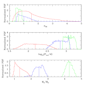
Figure 1: Distributions in the possible primary progenitor mass at the start of the CE phase ($M_{1}$, bottom panel), orbital period at the start of the CE phase, $P_{\mathrm{CE,i}}$, (middle panel) and the CE ejection efficiency, $\alpha_{\mathrm{CE}}$ (where we use $\lambda=\lambda_{\mathrm{g}}$; top panel) for SDSS2216+0102 (red), SDSS1548+4057 (blue) and for SDSS0303-0054 (green). The vertical lines indicate the mean values for each histogram.

Figure 2: Correlation matrix plot for the considered binary parameters. Rows correspond to independent variables, while columns correspond to dependent variables. Errors and numbers are omitted for clarity.

Fig. 1 shows distributions of possible primary progenitor mass at the start of the CE phase ($M_{1}$, bottom panel), orbital period at the onset of the CE phase ($P_{\mathrm{CE,i}}$, middle panel) and the CE ejection efficiency ($\alpha_{\mathrm{CE}}$, top panel, where we use $\lambda=\lambda_{\mathrm{g}}$) for SDSS2216+0102 (red), SDSS1548+4057 (blue) and SDSS0303-0054 (green). The vertical lines indicate the mean value for each histogram.

The white dwarf masses for SDSS2216+0102, SDSS1548+4057 and SDSS0303-0054 are $0.400\pm{0.060}$ M_⊙, $0.646\pm{0.032}$ M_⊙ and $0.912\pm{0.034}$ M_⊙ respectively. We can see from the bottom and middle panels that the average primary mass and orbital period immediately before the CE phase increase for increasing mass of the white dwarf descendant.

The orbital periods of these systems immediately after the CE phase are approximately the same ($\approx{0.2}$ d). Therefore, the typical progenitor of SDSS0303-0054 would need to spiral-in further during the CE phase than SDSS2216+0102 in order to reach the same post-CE orbital period. Therefore, for the former system, more orbital energy would be needed to eject the CE from the system than for the latter system. Hence, the typical ejection efficiency will be less efficient for SDSS0303-0054 than for SDSS2216+0102. This is illustrated by the histograms in the top panel. The average orbital separation and primary mass before the CE phase for SDSS1548+4057 lies between the average values for SDSS2216+0102 and SDSS0303-0054. Therefore, the average ejection efficiency for this system also lies between SDSS2216+0102 and SDSS0303-0054.

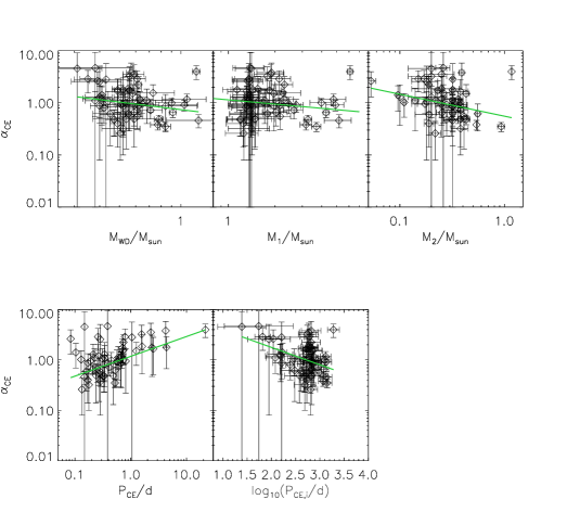
Figure 3: Our reconstructed values of $\alpha_{\mathrm{CE}}$ versus the following binary parameters, where we take $\lambda=\lambda_{\mathrm{g}}$: white dwarf mass, $M_{\mathrm{WD}}$; primary mass at the moment the CE phase commences, $M_{1}$; secondary mass, $M_{2}$; orbital period at the moment the CE ends, $P_{\mathrm{CE}}$; log₁₀ of the orbital period at the start of the CE phase, $P_{\mathrm{CE,i}}$. The solid green lines indicate linear fits to the data.

Figure 4: Our reconstructed values of $\alpha_{\mathrm{CE}}$ (y-axis, $\alpha_{\mathrm{CE}}(\mathrm{obs.})$) versus values of $\alpha_{\mathrm{CE}}$ (x-axis, $\alpha_{\rm{CE}}(\mathrm{mod.})$) which have been calculated from eqn. (14). Also shown is the value of the intercept and gradient of the linear fit through the data, which is shown as the solid black line.

Figure 5: Same as Fig. 5, except $\alpha_{\mathrm{CE}}(\mathrm{mod.})$ has been calculated from eqn. (15).

Table 1: A summary of the fit parameters $\epsilon_{0}$ and $\epsilon_{1}$ for the data in each panel of Fig. 3, where we consider $\lambda=\lambda_{\mathrm{g}}$. Also shown for each panel are the values of $\mathcal{F}$ and the probability of exceeding $\mathcal{F}$, $\mathscr{P}(\mathcal{F})$. Finally, an indication of whether we can reject the null hypothesis $\mathscr{H}^{\mathcal{F}}_{0}$ is included (see text for further details).

$Q$	$\epsilon_{0}$	$\epsilon_{1}$	$\mathcal{F}$	$\mathscr{P}(\mathcal{F})$	Reject $\mathscr{H}^{\mathcal{F}}_{0}$ ?$\,{}^{\mathrm{a}}$
$M_{\mathrm{WD}}$	-0.13$\pm$0.05	-0.48$\pm$0.27	3.2	$1\times{10}^{-1}$	No
$M_{1}$	0.06$\pm$0.09	-0.27$\pm$0.18	2.2	$1\times{10}^{-1}$	No
$M_{2}$	-0.26$\pm$0.08	-0.42$\pm$0.15	7.4	$9\times{10}^{-3}$	Yes
$P_{\mathrm{CE}}$	0.07$\pm$0.04	0.39$\pm$0.07	29.5	$<10^{-6}$	Yes
$P_{\mathrm{CE,i}}$	0.94$\pm$0.33	-0.34$\pm$0.11	9.1	4$\times{10}^{-3}$	Yes

^a $\mathcal{F}_{\mathrm{crit}}=4.00$ for a 0.05 significance level.

Table 2: A summary of our fit parameters, obtained from a multi-regression analysis of the values of $\alpha_{\mathrm{CE}}$ (where $\lambda=\lambda_{\mathrm{g}}$) as a function of two or more binary parameters. Shown are the coefficients $\beta_{0...m}$, the F-statistic, $\mathcal{F}$, and the probability of exceeding $\mathcal{F}$, $\mathscr{P}(\mathcal{F})$. We also indicate whether we can reject the null hypothesis $\mathscr{H}_{0}^{\mathcal{F}}$.

Variables	$\beta_{0}$	$\beta_{1}$	$\beta_{2}$	$\beta_{3}$	$\beta_{4}$	$\mathcal{F}$	$\mathscr{P}(\mathcal{F})$	Reject $\mathscr{H}_{0}^{\mathscr{F}}$ ?
Progenitor parameters
$P_{\mathrm{CE,i}}+M_{\mathrm{WD}}$	2.35	-0.78$\pm$0.25	1.09$\pm$0.56	-	-	3.6	6$\times{10}^{-2}$	No
$+M_{2}$	1.94	-0.67$\pm$0.27	1.04$\pm$0.56	-0.19$\pm$0.19	-	1.1	$3\times{10}^{-1}$	No
$+M_{1}$	1.88	-0.66$\pm$0.30	0.97$\pm$1.38	-0.20$\pm$0.20	0.04$\pm$0.72	$0.003$	$9.6\times{10}^{-1}$	No
Observable (PCEB) parameters
$P_{\mathrm{CE}}+M_{\mathrm{WD}}$	-0.03	0.20$\pm$0.03	-0.85$\pm$0.21	-	-	16.6	$2\times{10}^{-4}$	Yes
$+M_{2}$	-0.31	0.28$\pm$0.02	-0.95$\pm$0.13	-0.17$\pm$0.09	-	38.4	$<1\times{10}^{-6}$	Yes

2.4 Statistical Approach

Our aim in this investigation is to apply a chi-squared multi-regression analysis (via the Levenberg-Marquardt method) to obtain fits of $\alpha_{\mathrm{CE}}$ for two cases; we do this by first determining whether correlations exist between $\alpha_{\mathrm{CE}}$ and the binary progenitor parameters at the point that the CE phase commences (i.e. the moment the primary progenitor star just fills its Roche lobe), which will be useful for population synthesis calculations. In the second case, we determine whether correlations exist between $\alpha_{\mathrm{CE}}$ and the (observable) PCEB parameters, which may be a useful diagnostic to probe CE physics.

We proceed as follows. We fit our reconstructed values of $\alpha_{\mathrm{CE}}$ according to the equation

$$\mathrm{log}_{10}\alpha_{\mathrm{CE}}=\beta_{0}+\sum_{i=1}^{m}\beta_{i}\mathrm{log}_{10}Q_{i},$$ (11)

where $\beta_{0...m}$ are constants. If we are considering the progenitor binary parameters only, then $Q\in{\{P_{\mathrm{CE,i}},M_{2},M_{\mathrm{WD}},M_{1}\}}$, with $m=4$. If we consider the PCEB parameters, then $Q\in{\{P_{\mathrm{CE}},M_{2},M_{\mathrm{WD}}\}}$, with $m=3$.

Strictly speaking, we should only apply the Levenberg-Marquardt chi-squared method if the errors are normally distributed. As we can see from Fig. 1, this is not the case. We may therefore under-estimate the uncertainties in our fit parameters. To tackle this, we rescale the standard deviations for the values of $\alpha_{\mathrm{CE}}$ such that we obtain a reduced chi-squared value of 1.

To determine which variable to include first in our fit, we perform a 1-dimensional (1D) linear fit of our reconstructed values of $\alpha_{\mathrm{CE}}$ versus each of the binary parameters. Specifically, we fit the function of the form

$$\mathrm{log}_{10}\alpha_{\mathrm{CE}}=\epsilon_{0}+\epsilon_{1}\mathrm{log}Q,$$ (12)

where $\epsilon_{0}$ and $\epsilon_{1}$ are constants.

Then, to determine if a linear fit – as opposed to a constant fit – to the data is actually warranted (i.e. we reject the null hypothesis $\mathscr{H}_{0}^{\mathcal{F}}$), we perform the F-test (see Section B). We choose a significance level of $\alpha=0.05$. The first variable which we include in our fit is the one which gives the smallest probability, $\mathscr{P}(\mathcal{F})$, that we will obtain an F-statistic smaller than the obtained value, $\mathcal{F}$.

Once we have added our first variable to the fit, we determine the next binary parameter to include, by performing both a constant and a 1D fit to the residuals as a function of the remaining binary parameters. The next variable which we add is the one which gives the smallest value of $\mathscr{P}(\mathcal{F})$. In principle, we can repeat this process until we have a fit in terms of all binary parameters.

However, special care should be taken when performing regression-analysis; strictly speaking, the predictor variables should be independent of one another. We check whether there is any correlation between the binary parameters via a correlation matrix plot as shown in Fig. 2. There are clearly strong correlations between $M_{\mathrm{WD}}$, $M_{1}$ and $P_{\mathrm{CE,i}}$. This is to be expected because the core mass of a Roche lobe-filling star is a (weak) function of the total mass, and as a function of the orbital period via the star’s Roche lobe radius and Kepler’s Third Law. Hence, by including some or all of these variables we may over-fit the data, and we may render certain variables redundant in the fit.

As we add each variable to our fit as described above, we once again apply the $\mathcal{F}$-Test to determine whether the fit is a statistically better fit than the one without this added binary parameter.

Our results for the case with $\lambda=\lambda_{\mathrm{g}}$ and $\lambda=\lambda_{\mathrm{b}}$ are discussed in turn in the following Sections.

3 Results

The observed binary parameters (component masses and orbital period) as well as the cooling age of the white dwarf, $t_{\mathrm{cool}}$, are summarised in table 7 for PCEBs detected by the SDSS. Table 8 is the same but for PCEBs recorded in the Ritter & Kolb (2003) catalogue, Edition 7.14 (2010). The average values of $\alpha_{\mathrm{CE}}$, $P_{\mathrm{CE,i}}$ and $M_{1}$ and their standard deviations (calculated from distributions similar to those illustrated in Fig. 1) for each observed PCEB are also summarised in Table 7 and 8 where we do not consider the internal energy of the progenitor primary envelope. Tables LABEL:CERecon_SDSS_B and 10 give the average values of $M_{1}$, $P_{\mathrm{CE,i}}$ and $\alpha_{\mathrm{CE}}$ for each observed PCEB when we do consider the internal energy of the progenitor primary envelope.

3.1 For $\lambda=\lambda_{\mathrm{g}}$

Table 3: Same as Table 1 except for the data shown in Fig. 6.

$Q$	$\epsilon_{0}$	$\epsilon_{1}$	$\mathcal{F}$	$\mathscr{P}(\mathcal{F})$	Reject $\mathscr{H}^{\mathcal{F}}_{0}$ ?a
$M_{\mathrm{WD}}$	-1.03$\pm$0.10	-2.10$\pm$0.34	36.1	$<10^{-6}$	Yes
$M_{1}$	-0.21$\pm$0.07	-1.26$\pm$0.23	30.0	$<10^{-6}$	Yes
$M_{2}$	-0.89$\pm$0.13	-0.70$\pm$0.20	2.9	$6\times{10}^{-4}$	Yes
$P_{\mathrm{CE}}$	-0.45$\pm$0.06	0.15$\pm$0.10	2.7	$1\times{10}^{-1}$	No
$P_{\mathrm{CE,i}}$	1.55$\pm$0.43	-0.76$\pm$0.16	22.4	$2\times{10}^{-5}$	Yes

^a $\mathcal{F}_{\mathrm{crit}}=4.00$ for a 0.05 significance level.

Table 4: The same as Table 2 except now for our data calculated using $\lambda_{\mathrm{b}}$.

Variables	$\beta_{0}$	$\beta_{1}$	$\beta_{2}$	$\beta_{3}$	$\beta_{4}$	$\mathcal{F}$	$\mathscr{P}(\mathcal{F})$	Reject $\mathscr{H}_{0}^{\mathscr{F}}$ ?
Progenitor parameters
$M_{\mathrm{WD}}+M_{2}$	-1.08	-1.94$\pm$0.29	-0.14$\pm$0.14	-	-	0.4	0.5	No
$+P_{\mathrm{CE,i}}$	-0.54	-1.65$\pm$0.39	-0.13$\pm$0.15	-0.17$\pm$0.16	-	0.6	0.4	No
$+M_{1}$	0.98	0.22$\pm$1.26	-0.07$\pm$0.15	-0.46$\pm$0.24	-0.98$\pm$0.63	1.1	0.3	No
Observable (PCEB) parameters
$M_{\mathrm{WD}}+P_{\mathrm{CE}}$	-1.18	-3.20$\pm$0.26	0.22$\pm$0.03	-	-	71.8	$<{10}^{-6}$	Yes
$+M_{2}$	-1.53	-2.50$\pm$0.16	0.31$\pm$0.02	-1.02$\pm$0.09	-	127.5	$<{10}^{-6}$	Yes

Our values of $\alpha_{\mathrm{CE}}$ versus $M_{\mathrm{WD}}$, $M_{1}$, $M_{2}$, $P_{\mathrm{CE}}$ and $P_{\mathrm{CE,i}}$ are shown in Fig. 3 for the case where we consider $\lambda=\lambda_{\mathrm{g}}$. Each point corresponds to the mean value of $\alpha_{\mathrm{CE}}$, while the vertical lines correspond to the standard deviation.

The values of $\epsilon_{0}$, $\epsilon_{1}$ for each panel of Fig. 3 are given in Table 1. The solid green curves in Fig. 3 are the linear fits. For comparison, we also fit a constant function to the data in Figs. 3 of the form

$$\mathrm{log}_{10}\alpha_{\mathrm{CE}}=\epsilon_{0},$$ (13)

where $\epsilon_{0}$ is a constant. For the data in Fig. 3, we find that $\epsilon_{0}=-0.06\pm 0.04$.

Values of $\mathcal{F}$ [and the probability that we exceed this value, $\mathscr{P}(\mathcal{F})$] for the data in Fig. 3 are given in Table 1. Table 1 also indicates whether we can reject the null hypothesis $\mathscr{H}^{\mathcal{F}}_{0}$ (see Section B).

3.1.1 A fit in terms of the progenitor parameters

Table 1 indicates that we can reject $\mathscr{H}_{0}^{\mathcal{F}}$ for $P_{CE,i}$ and $M_{2}$. The first variable which we add to our fit is $P_{\mathrm{CE,i}}$ as this has the smallest value of $\mathscr{P}(\mathcal{F})$. Subsequent variables which we add, and the corresponding fit parameters, are summarised in the top panel of Table 2. Specifically, Table 2 gives the values $\beta_{0...m}$, the F-statistic $\mathcal{F}$ and $\mathscr{P}(\mathcal{F})$. We also indicate whether we can reject $\mathscr{H}_{0}^{\mathcal{F}}$ for each fit. We adopt a significance level of 0.05.

We find that adding binary parameters in addition to $P_{\mathrm{CE,i}}$ do not provide an improved fit over one in terms of $P_{\mathrm{CE,i}}$ only. Indeed, $\mathscr{P}(\mathcal{F})>0.05$ in all cases. For such fits, we therefore cannot reject $\mathscr{H}_{0}^{\mathcal{F}}$. Hence, we find the following fit of $\alpha_{\mathrm{CE}}$ in terms of $P_{\mathrm{CE,i}}$ which is given by

$$\mathrm{log}_{10}\alpha_{\mathrm{CE}}=(0.94\pm 0.33)-(0.34\pm 0.11)\mathrm{log}_{10}\left(\frac{P_{\mathrm{CE,i}}}{\mathrm{d}}\right).$$ (14)

Our reconstructed values of $\alpha_{\mathrm{CE}}$ versus values calculated from equation (14) are shown in Fig. 5.

3.1.2 A fit in terms of the PCEB parameters

The first variable which we add to our fit is $P_{\mathrm{CE}}$. Subsequent variables that we add, and the corresponding fit parameters, are summarised in the bottom panel of Table 2. In contrast to our fit of $\alpha_{\mathrm{CE}}$ in terms of the progenitor parameters, we find that adding $M_{\mathrm{WD}}$ and then $M_{2}$ is an improvement over the fit which is only in terms of $P_{\mathrm{CE}}$; we have $\mathcal{F}=16.6$ and 38.4 for the former and latter cases respectively. Hence, we can reject $\mathscr{H}_{0}^{\mathcal{F}}$ for both of these alternative fits. Hence, we suggest

$$\mathrm{log}_{10}{\alpha_{\mathrm{CE}}}=-0.31-(0.95\pm 0.13)\mathrm{log}_{10}\left(\frac{M_{\mathrm{WD}}}{\mathrm{M}_{\odot}}\right)$$

$$+(0.28\pm 0.02)\mathrm{log}_{10}\left(\frac{P_{\mathrm{CE}}}{\mathrm{d}}\right)$$

$$-(0.17\pm 0.09)\mathrm{log}_{10}\left(\frac{M_{2}}{\mathrm{M}_{\odot}}\right).$$ (15)

Fig. 5 is the same as Fig. 5 except equation (15) is used.

3.2 For $\lambda=\lambda_{\mathrm{b}}$

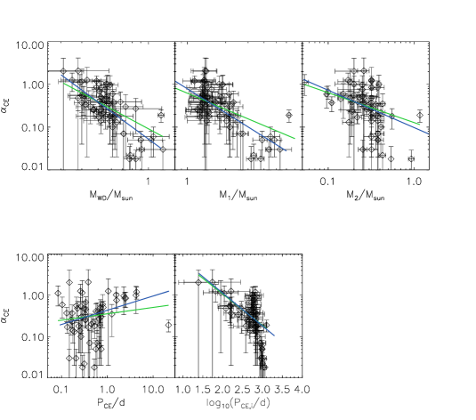
Figure 6: Similar to Fig. 3 except for the case where we take $\lambda=\lambda_{\mathrm{b}}$. The solid blue lines indicate linear fits to the data using the bootstrapping technique (see Section 4 for further details).

The reconstructed values of $\alpha_{\mathrm{CE}}$ versus each binary parameter are shown in the corresponding panels in Fig. 6. The values of $\epsilon_{0}$, $\epsilon_{1}$ are summarised in Table 3, as are the $\mathcal{F}$-statistics, and whether we can reject $\mathscr{H}_{0}^{\mathcal{F}}$. For comparison with our linear fits, we once again perform a constant fit to our values of $\alpha_{\mathrm{CE}}$ in the form of eqn. (13).We find that $\epsilon_{0}=-0.49\pm 0.05$.

3.2.1 A fit in terms of the progenitor parameters

Table 3 indicates that we can reject $\mathscr{H}_{0}^{\mathcal{F}}$ for the 1D fit of $\alpha_{\mathrm{CE}}$ versus $M_{\mathrm{WD}}$, $M_{1}$, $M_{2}$ or $P_{\mathrm{CE,i}}$. We obtain the smallest value of $\mathscr{P}(\mathcal{F})$ for $M_{\mathrm{WD}}$, and so this is the first binary parameter we add to our fit. Subsequent additions and the corresponding fit parameters are summarised in the top panel of Table 4, which shows the same quantities as displayed in Table 2.

Adding more binary parameters to our fit does not provide an improvement over the fit only in terms of $M_{\mathrm{WD}}$. This is probably a result of the fact that trends exist between $M_{1}$, $M_{\mathrm{WD}}$ and $P_{\mathrm{CE,i}}$. Therefore, we suggest a fit of $\alpha_{\mathrm{CE}}$ as a function of $M_{\mathrm{WD}}$ only, i.e.

$$\mathrm{log}_{10}\alpha_{\mathrm{CE}}=(-1.03\pm 0.10)-(2.10\pm 0.34)\mathrm{log}_{10}\left(\frac{M_{\mathrm{WD}}}{\mathrm{M}_{\odot}}\right).$$ (16)

Fig. 8 is the same as Fig. 5 except equation (16) is used.

3.2.2 A fit in terms of the PCEB parameters

We once again start with $M_{\mathrm{WD}}$ in our fit, with the fit parameters for additional variables summarised in the bottom panel of Table 4. Including $P_{\mathrm{CE}}$ and then $M_{2}$ provides an improved fit over one in terms of $M_{\mathrm{WD}}$ only; we can reject $\mathscr{H}_{0}^{\mathcal{F}}$ in either case. As for the case where $\lambda=\lambda_{\mathrm{g}}$, we suggest a fit of $\alpha_{\mathrm{CE}}$ as a function of $M_{\mathrm{WD}}$, $M_{2}$ and $P_{\mathrm{CE}}$, given by

$$\mathrm{log}_{10}{\alpha_{\mathrm{CE}}}=-1.18-(2.50\pm 0.16)\mathrm{log}_{10}\left(\frac{M_{\mathrm{WD}}}{\mathrm{M}_{\odot}}\right)$$

$$+(0.31\pm 0.02)\mathrm{log}_{10}\left(\frac{P_{\mathrm{CE}}}{\mathrm{d}}\right)$$

$$-(1.02\pm 0.09)\mathrm{log}_{10}\left(\frac{M_{2}}{\mathrm{M}_{\odot}}\right).$$ (17)

Fig. 8 is the same as Fig. 5 except equation (17) is used.

4 Discussion

We have found statistical evidence that the CE ejection efficiency has at least a first order dependence on the white dwarf mass, the progenitor primary mass, the secondary mass or the orbital period at the point the CE phase commences if we consider the case where $\lambda=\lambda_{\mathrm{b}}$. For $\lambda=\lambda_{\mathrm{g}}$, we find correlations between $\alpha_{\mathrm{CE}}$ and $M_{2}$, $P_{\mathrm{CE}}$ or $P_{\mathrm{CE,i}}$. However, whether we consider $\lambda=\lambda_{\mathrm{g}}$ or $\lambda=\lambda_{\mathrm{b}}$, we do not obtain a statistically significant fit of $\alpha_{\mathrm{CE}}$ in terms of more than one progenitor binary parameter.

This behaviour may be a result of the large uncertainties of the progenitor system parameters for a given observed PCEB. As Fig. 1 demonstrates, an uncertainty for the white dwarf mass of a few$\times 0.01$ M_⊙ can translate into possible progenitor primary masses that span between approximately 1 and 2 M_⊙, or into a pre-CE orbital period that can range from a few hundred to approximately 1000 d. As Tables 7 to 10 show, this can result in a standard deviation in $\alpha_{\mathrm{CE}}$ as large as approximately 100 per cent of the mean value. This presents a challenge to efforts aimed at discerning potentially small, albeit real, trends with binary parameters.

Even if the trends which we see are statistically significant, it is unclear whether they have a physical underpinning. The initial distribution functions which we use to weight the possible values of $\alpha_{\mathrm{CE}}$ for a given PCEB have been inferred from binary populations which may be prone to selection effects. Hence, for a given observed system, the calculated average value of $\alpha_{\mathrm{CE}}$ may not be the true average $\alpha_{\mathrm{CE}}$.

We now address whether there is a source of energy in addition to gravitational energy which is used during the ejection of the CE. We find that if we do consider the internal energy of the progenitor primary envelope, then this does bring the ejection efficiencies within the canonical range of $0<\alpha_{\mathrm{CE}}\leq{1}$, in agreement with Zorotovic et al. (2010) and as predicted by Webbink (2008). However, we still find that $\alpha_{\mathrm{CE}}\ga{1}$ for PCEBs with brown dwarf secondaries ($M_{2}\leq{0.1}$ M_⊙).

There is some debate as to what extent the internal energy of the giant’s envelope plays a role in the ejection of the CE. Indeed, Harpaz (1998) argues that during the planetary nebula phase, the opacity of the giant’s hydrogen ionization zone decreases during recombination. Hence, the envelope becomes transparent to its own radiation. The radiation will therefore freely escape rather than push against the material to eject it. On the other hand, Webbink (2008) argues that the ionization zone of giant and AGB stars is buried beneath a region of the envelope whose opacity is dominated by heavy elements. Once recombination is triggered at the onset of the CE phase, the escaping radiation can therefore ‘push’ against these high-opacity layers.

Ivanova & Chaichenets (2011), on the other, suggest that the enthalpy of the primary giant’s envelope, as opposed to the internal energy of the gas, should be considered. Indeed, they found that there exists a region in the giant interior, coined the ‘boiling pot zone’, where the enthalpy is greater than the gravitational potential. This excess of energy may cause an outflow of material lying above the boiling-pot zone, and hence facilitate the ejection of the CE from the system. They find that by considering the enthalpy of the progenitor giant permits the formation of low-mass X-ray binaries with a low-mass companion, without resorting to $\alpha_{\mathrm{CE}}>1$.

Figure 7: Same as Fig. 5, except $\alpha_{\mathrm{CE}}(\mathrm{mod.})$ has been calculated from eqn. (16).

Figure 8: Same as Fig. 5, except $\alpha_{\mathrm{CE}}(\mathrm{mod.})$ has been calculated from eqn. (17).

Our calculations with $\lambda=\lambda_{\mathrm{b}}$ assume that all of the internal energy of the envelope is used to unbind the CE from the system, i.e $\alpha_{\mathrm{th}}=1$ in eqn. (5), which is clearly unrealistic. Nonetheless, by reconstructing the CE phase with and without consideration for the internal energy of the primary envelope, we provide upper and lower limits for $\alpha_{\mathrm{CE}}$. Furthermore, our reconstructed values of $\alpha_{\mathrm{CE}}$ and their trends with binary parameters presented in Section 3 will provide useful constraints on detailed models of the CE microphysics.

Another result to note from our investigation regards the progenitors of those PCEBs with high mass white dwarfs. For PCEBs with white dwarf masses $M_{\mathrm{WD}}\ga 0.7$ M_⊙, there are possible progenitor primaries which have $\lambda_{\mathrm{b}}<0$ at the onset of the CE phase (see also Section 2.3). The envelope is therefore unbound from the giant as a result of radiation pressure driven winds. A particularly striking example is IK Peg, where a vast majority of the possible progenitors have $\lambda_{\mathrm{b}}<0$ (see Fig. 9). This begs the question: did IK Peg really form via a CE phase? Dermine et al. (2009) investigated the effect that radiation pressure from giant stars has on the Roche lobe geometry. If $f$ is the ratio of the radiation to the gravitational force, they found that the critical Roche lobe around the donor star becomes meaningless if $f=1$. Hence, mass lost from the star will be in the wind regime, and material may not necessarily be channelled directly into the Roche lobe of the secondary star. Hence, in the context of giant stars, a situation where $f\geq 1$ may mean that a CE phase is avoided. Theoretical studies investigating this possibility need to be carried out further.

In the following Sections, we discuss important points regarding the reconstructed values of $\alpha_{\mathrm{CE}}$ versus each binary parameter in turn.

4.1 $\alpha_{\mathrm{CE}}$ versus $M_{\mathrm{WD}}$

The following argument may further help to explain why we can reject more frequently $\mathscr{H}^{\mathcal{F}}_{0}$ for the data calculated using $\lambda=\lambda_{\mathrm{b}}$ rather than when $\lambda=\lambda_{\mathrm{g}}$ is used. Recall that there are some PCEB progenitor primaries with $M_{\mathrm{WD}}\ga{0.7}$ M_⊙ which have $\lambda_{\mathrm{b}}<0$ (see Section 4). Furthermore, the progenitor primaries of these PCEBs which do have $\lambda_{\mathrm{b}}>0$ have very large values of $\lambda_{\mathrm{b}}$ (and a correspondingly small binding energies) owing to their large radii when they fill their Roche lobes at the start of the CE phase. As a result, $\alpha_{\mathrm{CE}}$ will be very small (for example IK Peg, where we find a mean CE ejection efficiency of $\alpha_{\mathrm{CE}}=0.19$). This explains why the values of $|\epsilon_{1}|$ are larger when we consider $\lambda=\lambda_{\mathrm{b}}$ than when we consider $\lambda=\lambda_{\mathrm{g}}$.

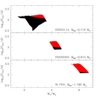
Figure 9: Two dimensional distributions in primary mass, $M_{1}$ and orbital period, $P_{\mathrm{CE,i}}$, at the very start of the CE phase, for three systems as indicated in the bottom right of each panel.Black points indicate that $\lambda_{\mathrm{b}}>0$ for those progenitors, while red data points indicate that $\lambda_{\mathrm{b}}<0$.

Furthermore, we find that as the white dwarf mass increases, the number of possible progenitor primaries with $\lambda_{\mathrm{b}}>0$ decreases. This is graphically illustrated in Fig. 9, which shows the two-dimensional distribution in $M_{1}$ and $P_{\mathrm{CE,i}}$ for three systems: SDSS2214-0103, SDSS0303-0054 and IK Peg. Black points indicate that $\lambda_{\mathrm{b}}>0$ for the associated progenitor, while red points indicate that $\lambda_{\mathrm{b}}<0$ for that progenitor.

This means that the range of possible progenitor primary masses, and orbital periods at the start of the CE phase, and consequently the range in $\alpha_{\mathrm{CE}}$ will decrease. As a result, the standard deviation in $\alpha_{\mathrm{CE}}$ will decrease. Such data points will therefore have a large weighting in the fits. The linear fits between $\alpha_{\mathrm{CE}}$ and $M_{\mathrm{WD}}$ may be greatly influenced by such data points.

To determine if this is the case, and to determine if a linear relationship does exist among the other data points, we perform a bootstrap analysis to the $\alpha_{\mathrm{CE}}$ versus $M_{\mathrm{WD}}$ data in Fig. 6. The mean value of $\epsilon_{1}$ and the standard error from this analysis is given in Table 5. The linear fit calculated from our bootstrapping analysis are shown in Fig. 6 as solid blue curves.

Table 5: The mean values with errors of the coefficient $\epsilon_{1}$ calculated from our bootstrapping analysis of the data in each panel of Fig. 6.

$Q$	$\epsilon_{1}$
$M_{\mathrm{WD}}$	-2.88$\pm$0.33
$M_{1}$	-1.87$\pm$0.28
$M_{2}$	-0.87$\pm$0.24
$P_{\mathrm{CE}}$	0.34$\pm$0.11
$P_{\mathrm{CE,i}}$	-0.79$\pm$0.15

In comparison to the linear fit, we find that the bootstrap analysis also indicates that $\alpha_{\mathrm{CE}}$ decreases with increasing $M_{\mathrm{WD}}$, albeit a slightly steeper (i.e. a more negative) value of $\epsilon_{1}$ is predicted. In other words, a marginally stronger linear relationship between $\alpha_{\mathrm{CE}}$ and $M_{\mathrm{WD}}$ is predicted by the bootstrapping analysis. By comparing the green and blue lines in Fig. 6 we can see that the data points at large white dwarf masses have the effect of flattening the gradient. The majority of the data points, however, suggest a steeper gradient.

4.2 $\alpha_{\mathrm{CE}}$ versus $M_{1}$

The linear fits to the corresponding panels in Fig. 3 and 6 suggest that $\alpha_{\mathrm{CE}}$ decreases with increasing $M_{1}$. This is in contrast to De Marco et al. (2011), who found that $\alpha_{\mathrm{CE}}$ increases with $M_{1}$. We explore this further in Section 5.2.

In light of the influence that data points corresponding to PCEBs with high mass white dwarfs may have on the fitting (see Section 4.1) we also perform a bootstrapping analysis on the $M_{1}$ versus $\alpha_{\mathrm{CE}}$ data in Fig. 6. (We repeat this analysis for the subsequent binary parameters in our discussion). Our bootstrap analysis predicts a slightly more negative value than the value obtained from the chi-squared fit. Therefore, those data points corresponding to high mass white dwarfs do not significantly affect the linear fit.

4.3 $\alpha_{\mathrm{CE}}$ versus $M_{2}$

We find that $\alpha_{\mathrm{CE}}$ decreases with increasing $M_{2}$, irrespective of whether we use $\lambda_{\mathrm{g}}$ or $\lambda_{\mathrm{b}}$. This finding is in agreement with De Marco et al. (2011), but in contrast to the suggestion made by Politano & Weiler (2007), who proposed that $\alpha_{\mathrm{CE}}$ may increase with increasing $M_{2}$.

This suggestion was motivated by the fact that very few, if any, CVs with brown dwarf secondaries at orbital periods below 77 min have been detected. This appeared to be in conflict with Politano (2004) who estimated from his models that such systems should make up approximately 15 per cent of the total CV population (see also Kolb & Baraffe, 1999). Politano (2004) suggested that this discrepancy may be a result of the decreasing energy dissipation rate of orbital energy within the CE for decreasing secondary mass, and that below some cut-off mass, a CE merger would be unavoidable. Indeed, the small surface area of the secondary star will generate a correspondingly small friction force with the CE material. Also, as can be seen from eqn. (6), the change in orbital energy during spiral-in will be small for small secondary masses.

However, as PCEBs with $M_{2}\la{0.1}$ M_⊙ are observed, the CE ejection must be very efficient if such systems are to avoid a merger. De Marco et al. (2011) suggested this may be achieved if smaller mass components take longer than the giant’s dynamical time to penetrate into the envelope. The giant star would therefore have time to thermally re-adjust its structure, and use this thermal energy to aid the ejection of the CE. Note, however, that systems with secondaries $M_{2}\approx{0.1}$ M_⊙ (see Fig. 6), require a mean ejection efficiency close to 1, even if we consider the internal energy of the progenitor primary’s envelope.

The bootstrap analysis yields only a marginally steeper gradient than that obtained from the chi-squared fit.

4.4 $\alpha_{\mathrm{CE}}$ versus $P_{\mathrm{CE}}$

We find that $\alpha_{\mathrm{CE}}$ increases with increasing $P_{\mathrm{CE}}$, irrespective of whether we consider the internal energy of the progenitor primaries or not.

Furthermore, the orbital separation at the point the CE terminates, $A_{\mathrm{CE,f}}$ (found via $P_{\mathrm{CE}}$), for the observed PCEBs indicates how deep the secondary star penetrated into the envelope of the giant star by the time the CE ceased. This may shed further light into the role that the structure of the giant primary plays during the termination of the CE phase. Yorke et al. (1995) suggested that a steep decrease in density within the giant star is required for the successful termination of the CE phase. Such a decrease is characterized by a flat mass-radius profile of the star.

Once the secondary star reaches this region, the energy dissipation rate within the CE decreases, and the CE phase comes to an end, provided that the envelope material exterior to this region has been unbound from the system. Terman & Taam (1996) suggest that the values of $A_{\mathrm{CE,f}}$ for PCEBs may be estimated from the location within the CE where the mass-radius profile is no longer flat, i.e. when the quantity $V=\mathrm{d}\,\mathrm{ln}P/\mathrm{d}\,\mathrm{ln}r$ is at a minimum. Here, $P$ is the pressure and $r$ is the radial coordinate.

Terman & Taam (1996) found from their hydrodynamical simulations that the orbital separation of PCEBs immediately after the CE phase was proportional to the white dwarf mass (see their Fig. 8), as a consequence of the fact that the point where $V$ is minimum moves further away from the stellar centre for more evolved stars. Therefore, a plot of $M_{\mathrm{WD}}$ versus $A_{\mathrm{CE,f}}$ for our observed sample of PCEBs would provide an excellent comparison with the aforementioned theoretical study.

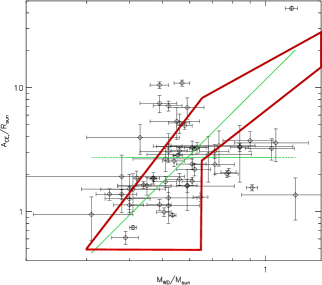
Figure 10: A plot of white dwarf mass versus the post-CE orbital separation for our observed sample of PCEBs. The green dotted line is a constant fit to the data, while the green solid line is a linear fit to the data. The thick red border outlines the approximate region in $A_{\mathrm{CE,f}}-M_{\mathrm{WD}}$ space inhabited by the data points given in Fig. 8 of Terman & Taam (1996), calculated from their hydrodynamical simulations.

Such a plot is shown in Fig. 10. To determine if a linear relationship between $M_{\mathrm{WD}}$ and $A_{\mathrm{CE,f}}$ does exist, we fit a linear function given by

$$\mathrm{log}_{10}A_{\mathrm{CE,f}}=\epsilon_{0}+\epsilon_{1}\mathrm{log}_{10}M_{\mathrm{WD}},$$ (18)

where $A_{\mathrm{CE,f}}$ is expressed in solar radii, and $M_{\mathrm{WD}}$ is expressed in solar masses. We find $\epsilon_{0}=1.07\pm 0.01$ and $\epsilon_{1}=2.76\pm 0.03$. For our value of the number of degrees of freedom, $\nu_{\mathrm{linr}}=58$, we therefore obtain a reduced chi-squared value of $\chi^{2}_{\mathrm{linr}}=98.62$. This curve is shown as the green solid line in Fig. 10. For comparison, we also show a constant fit to the data, $\mathrm{log}_{10}A_{\mathrm{CE,f}}=\epsilon_{0}$, where $\epsilon_{0}=0.435\pm 0.004$, and $\chi^{2}_{\mathrm{const}}=213.39$ (reduced), for $\nu_{\mathrm{const}}=59$ degrees of freedom.

The chi-squared values indicate that a linear function provides a better fit to the data in Fig. 10 than a constant one. To determine whether an extra parameter is warranted, we once again apply the F-Test. For our values of $\nu_{\mathrm{linr}}$ and $\nu_{\mathrm{cons}}$, we obtain $\mathcal{F}=67.5$ with $\mathscr{P}(\mathcal{F})<10^{-6}$. Hence, because $\mathscr{P}(\mathcal{F})<\alpha$, we can reject $\mathscr{H}^{\mathcal{F}}_{0}$. We therefore find intriguing statistical evidence that there is a functional dependence between $M_{\mathrm{WD}}$ and $A_{\mathrm{CE,f}}$.

The thick red border in Fig. 10 indicates the region in the $A_{\mathrm{CE,f}}-M_{\mathrm{WD}}$ plane inhabited by the data points in Fig. 8 of Terman & Taam (1996), calculated from their hydrodynamical simulations. It can be seen that there is reasonable overlap between the observed PCEB sample and the results of Terman & Taam (1996) for $M_{\mathrm{WD}}\la{0.7}$ M_⊙. In contrast, their simulations over-estimate the final orbital separation by as large as a factor of about 3 for systems with more massive white dwarf primaries.

However, as noted by Yorke et al. (1995), the orbital separation when the CE terminates does not necessarily coincide exactly with the point when $V$ becomes a minimum. Yorke et al. (1995) and Terman & Taam (1996) estimate that the orbital separation at which the orbital decay sufficiently decreases is approximately 3 to 10 times smaller than the distance when $V$ becomes a minimum. Terman & Taam (1996) assume a factor of one sixth of this distance in their Fig. 8, although it is more likely that this factor will differ from system to system.

More recently, Ivanova (2011) discussed the idea of the ‘compression point’ within the primary giant, and the role that this may play during the CE ejection phase. The compression point is the location within the giant primary star where the value $P/\rho$ (here $P$ is the pressure and $\rho$ is the density) is at a maximum. Ivanova (2011) found that, if the companion star is sufficiently massive, the envelope will be unbound up to the mass coordinate corresponding to the location of the compression point. Hence, the final orbital separation at the end of the CE phase may correspond with the radial coordinate associated with the compression point. Hence, our fit here may provide a useful diagnostic of the termination of the CE phase.

4.5 $\alpha_{\mathrm{CE}}$ versus $P_{\mathrm{CE,i}}$

The data points at high values of log${}_{10}(P_{\mathrm{CE,i}}/\mathrm{d})$ in Fig. 6 may overly influence the linear fits. The reason is the same as for those data points at high white dwarf masses, as discussed in Section 4.1: primaries that fill their Roche lobes towards longer orbital periods will have very large or negative values of $\lambda_{\mathrm{b}}$. Fewer progenitor systems will therefore have $\lambda_{\mathrm{b}}>0$, decreasing the range in possible values of $\alpha_{\mathrm{CE}}$.

We also find that the difference between $\epsilon_{1}$ calculated from the chi-squared fit and our bootstrap calculation is negligible; our bootstrap analysis gives a slightly steeper value of $\epsilon_{1}$ compared with that obtained from the chi-squared fit.

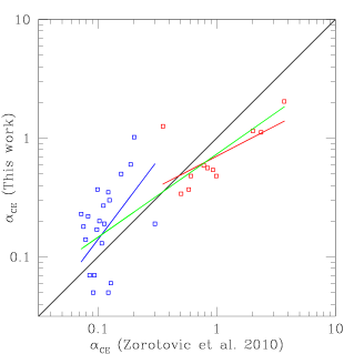
Figure 11: A comparison of our reconstructed values of $\alpha_{\mathrm{CE}}$ (y-axis) with those calculated by Zorotovic et al. (2010) (x-axis). PCEBs formed only from a primary progenitor on the first giant branch are indicated by the red points, while blue points indicate that the progenitor primary was on the AGB. The solid black line is of the form $\alpha_{\mathrm{CE}}$(this work)$=$$\alpha_{\mathrm{CE}}$(Zorotovic et al., 2010). Fits to the red and blue data points are shown as the red and blue lines respectively, while the green solid line is a linear fit to all the data points. Here, and in Figs. 12 and 13, error-bars are omitted for clarity.

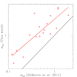
Figure 12: Similar to Fig. 11 except here we compare our values of $\alpha_{\mathrm{CE}}$ with those calculated by De Marco et al. (2011) (red data points).

5 Comparisons with previous studies

5.1 Comparisons with Zorotovic et al. (2010)

Fig. 11 compares our values of $\alpha_{\mathrm{CE}}$ calculated with $\lambda=\lambda_{\mathrm{b}}$ (y-axis) with those values calculated by Zorotovic et al. (2010) (x-axis). The black line indicates $y=x$.

For a given PCEB, Zorotovic et al. (2010) determine mean values of $\alpha_{\mathrm{CE}}$ separately from progenitors that commenced the CE phase on either the first giant branch (FGB) or on the AGB. Hence, Zorotovic et al. (2010) provide two mean values of $\alpha_{\mathrm{CE}}$ for some PCEBs. This is in contrast to the present investigation, where we calculate one mean value of $\alpha_{\mathrm{CE}}$ for each PCEB, from all possible progenitors.

Therefore, to place our comparison in Fig. 11 on an equal footing, we only compare values of $\alpha_{\mathrm{CE}}$ for systems that only have FGB progenitors (shown as red points in Fig. 11) and for systems with only AGB progenitors (blue points). The red and blue solid lines are linear fits to the corresponding data points, while the green curve is a fit to all the data points.

For the case of those systems which have AGB progenitors, we typically obtain larger values of $\alpha_{\mathrm{CE}}$ than Zorotovic et al. (2010), by no more than a factor of 2. For PCEBs with FGB progenitors, we typically get values of $\alpha_{\mathrm{CE}}$ which are smaller by a factor of no more than about 3.

While in this present work we always take $\alpha_{\mathrm{th}}=1$, Zorotovic et al. (2010) assume that the efficiency of using the giant envelope’s internal energy to eject the CE is equal to the efficiency of using the orbital energy. Their values of $\lambda$ are then calculated from this assumption. Furthermore, Zorotovic et al. (2010) calculate their values of $\lambda$ using analytical fits to the values of $E_{\mathrm{bind}}$, calculated from the stellar models of Pols et al. (1998). This is in contrast to the tabulated values of $\lambda_{\mathrm{b}}$ for $\alpha_{\mathrm{th}}=1$ used in the present investigation.

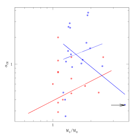
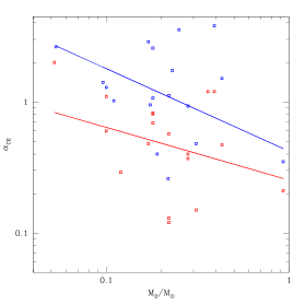
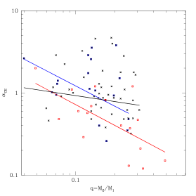
Figure 13: Reconstructed values of $\alpha_{\mathrm{CE}}$ versus $M_{1}$ (top left), $M_{2}$ (top right) and the mass ratio $q=M_{2}/M_{1}$ (bottom middle). Blue data points correspond to our values, while red points have been calculated by De Marco et al. (2011). The black crosses in the bottom panel are our entire PCEB sample. The lines of best-fit are shown as the blue, red and black lines respectively. The dotted blue line in the top panel is a best fit to our data but with V471 Tau (indicated by the arrow) omitted from the fit.

Table 6: Linear fit parameters for the data shown in the top-left, top-right and bottom panels of Fig. 13.

Study	$\epsilon_{0}$	$\epsilon_{1}$	$\chi^{2}_{\mathrm{linr}}$	$\chi^{2}_{\mathrm{cons}}$	$\mathcal{F}$	$\mathscr{P}(\mathcal{F})$	Reject $\mathscr{H}_{0}^{\mathcal{F}}$
$\alpha_{\mathrm{CE}}$ versus $M_{1}$
De Marco et al. (2011)	-0.41$\pm$ 0.09	0.73$\pm$ 0.42	16.28	19.32	3.0	0.1	No
This work (overlapping systems)	0.32$\pm$0.15	-1.16$\pm$0.40	34.07	52.09	8.5	0.01	Yes
This work (no V471 Tau)	0.01$\pm$0.17	0.56$\pm$0.74	23.34	24.24	0.6	0.5	No
$\alpha_{\mathrm{CE}}$ versus $M_{2}$
De Marco et al. (2011)	-0.59$\pm$0.22	-0.40$\pm$0.30	17.43	19.32	1.7	0.2	No
This work (overlapping systems)	-0.37$\pm$0.12	-0.63$\pm$0.19	30.28	52.09	11.5	0.004	Yes
$\alpha_{\mathrm{CE}}$ versus $q$
De Marco et al. (2011)	-0.97$\pm$0.22	-0.84$\pm$0.27	12.00	19.32	9.8	0.006	Yes
This work (overlapping systems)	-0.73$\pm$0.27	-0.82$\pm$0.31	36.48	52.09	6.8	0.02	Yes
This work (all systems)	-0.28$\pm$0.16	-0.24$\pm$0.17	136.41	141.22	2.0	0.2	No

5.2 Comparisons with De Marco et al. (2011)

We now compare our values of $\alpha_{\mathrm{CE}}$, calculated using $\lambda=\lambda_{\mathrm{g}}$, with those found by De Marco et al. (2011) in Fig. 12, for PCEBs that are common to both studies.

Fig. 12 indicates that we obtain larger values of $\alpha_{\mathrm{CE}}$ by between a factor of 2 and 3. Reasons for this disparity may be as follows. Firstly, De Marco et al. (2011) use an alternative expression for the envelope binding energy, given by the left-hand side of their eqn. 6 which, for a given progenitor primary giant, will give a smaller binding energy than that given by the left hand side of the Webbink (1984) formalism (c.f. our eqn. 3). Hence, for a given PCEB progenitor, a smaller value of $\alpha_{\mathrm{CE}}$ will be given if the De Marco et al. (2011) formalism is used. Secondly, our values of $\lambda_{\mathrm{g}}$ are calculated from both the mass and radius of the progenitor giant, while De Marco et al. (2011) calculate their values purely from the mass of the progenitor on the ZAMS. Hence, their method does not take into account any variations of $\lambda$ due to the location of the star (of a given mass) along the FGB or AGB, although they find that such variations are small.

De Marco et al. (2011) found that $\alpha_{\mathrm{CE}}$ increases with increasing $M_{1}$ but decreases with increasing $M_{2}$. Hence, they find that $\alpha_{\mathrm{CE}}$ decreases with increasing mass ratio, $q=M_{2}/M_{1}$, from their PCEB sample.

Fig. 13 shows data points on the $\alpha_{\mathrm{CE}}$-$M_{1}$ plane (top left panel), the $\alpha_{\mathrm{CE}}$-$M_{2}$ plane (top right panel) and on the $\alpha_{\mathrm{CE}}$-$q$ plane (bottom middle panel). Blue data points have been calculated in this present study, while red points have been calculated by De Marco et al. (2011), again for the aforementioned overlapping sample of PCEBs. The lines of best fit are shown as the blue and red lines respectively.

The fit parameters to the data in each panel is summarised in Table 6, as are the (unreduced) chi-squared values, $\chi^{2}_{\mathrm{linr}}$ and $\chi^{2}_{\mathrm{cons}}$, along with $\mathcal{F}$ and $\mathscr{P}(\mathcal{F})$. We also indicate whether we can reject $\mathscr{H}_{0}^{\mathcal{F}}$. The top-left panel of Fig. 13 shows that, in contrast to De Marco et al. (2011), a linear fit to our data suggests a decreasing $\alpha_{\mathrm{CE}}$ with increasing $M_{1}$. However, the data point indicated by the arrow (which corresponds to V471 Tau) may be overly influencing the fit. Indeed, the standard deviation in $\alpha_{\mathrm{CE}}$ for V471 Tau is the smallest in the sub-sample. A linear fit to the PCEB sub-sample without V471 Tau is given by the dotted blue line in the top-left panel of Fig. 13. This is now consistent with the fit obtained by De Marco et al. (2011). However, as Table 6 shows, we cannot reject $\mathscr{H}_{0}^{\mathcal{F}}$.

On the other hand, the trends obtained from the linear fits to the blue data points in the top-right and bottom panels are in line with those found by De Marco et al. (2011). We see that we obtain a very good agreement with De Marco et al. (2011) for the value of $\epsilon_{1}$ in the $\alpha_{\mathrm{CE}}$-$q$ plane. Here, we can also reject $\mathscr{H}_{0}^{\mathcal{F}}$ for both the red and blue data point on the $\alpha_{\mathrm{CE}}-q$ plane.

However, if we now perform a linear fit to our entire PCEB sample on the $\alpha_{\mathrm{CE}}-q$ plane (shown as the black crosses in the bottom panel of Fig. 13 and the black line respectively), then a trend between $\alpha_{\mathrm{CE}}$ and $q$ becomes less convincing. Indeed, we can no longer reject $\mathscr{H}_{0}^{\mathcal{F}}$. It is therefore uncertain whether the trend seen by De Marco et al. (2011) is physical, or whether it is due to the small PCEB sample which they used.

6 Conclusions

We reconstruct the common envelope (CE) phase for the current sample of post-common envelope binaries (PCEBs) with observationally determined component masses and orbital periods. We perform multi-regression analysis on our reconstructed values of the CE ejection efficiency, $\alpha_{\mathrm{CE}}$, in order to search for correlations between $\alpha_{\mathrm{CE}}$ and the binary parameters (both the progenitor and observed parameters). This analysis is carried out with and without consideration for the internal energy of the progenitor giants’ envelope.

If the internal energy of the progenitor giants’ envelope is taken into account, a statistically significant correlation (in terms of the progenitor parameters) is found between $\alpha_{\mathrm{CE}}$ and the white dwarf mass, $M_{\mathrm{WD}}$, only. We find that $\alpha_{\mathrm{CE}}$ decreases with increasing $M_{\mathrm{WD}}$.

If we do not consider the envelopes’ internal energy, we find the most statistically significant correlation exists between $\alpha_{\mathrm{CE}}$ and the orbital period at the start of the CE phase, $P_{\mathrm{CE,i}}$. Specifically, we find that $\alpha_{\mathrm{CE}}$ decreases with increasing $P_{\mathrm{CE,i}}$. In terms of the PCEB parameters, whether we consider the internal energy or not, we find a significant correlation between $\alpha_{\mathrm{CE}}$ and $M_{\mathrm{WD}}$, the orbital period immediately after the CE phase, $P_{\mathrm{CE}}$ and the secondary mass, $M_{2}$. While our values of $\alpha_{\mathrm{CE}}$, and the aforementioned correlations, cannot make definite physical claims regarding the CE phase, they will be nonetheless useful to constrain the micro-physics modelled in detailed CE simulations.

We re-iterate that uncertainties in the measured white dwarf masses result in uncertainties in the progenitor binary parameters, and in turn the values of $\alpha_{\mathrm{CE}}$. Future investigations into reconstructing the CE phase would therefore greatly benefit from more accurate determinations of PCEB white dwarf masses, for example from eclipsing systems.

If the internal energy of the progenitor primary envelope is considered, this brings the values of $\alpha_{\mathrm{CE}}$ more in line with the canonical range of $0<\alpha_{\mathrm{CE}}\leq{1}$. However, we still require $\alpha_{\mathrm{CE}}\ga 1$ to account for PCEBs with brown dwarf secondaries, i.e. with $M_{2}\la{0.1}$ M_⊙.

Finally, a large majority of possible progenitor primaries of IK Pegasi will have envelopes that have a positive binding energy. We suggest that IK Peg may have avoided the CE phase, and instead mass was lost from the system via radiation pressure driven winds.

Appendix A Initial distribution functions

We use three standard distribution functions to calculate the formation probability of the zero-age main sequence binary system. The initial mass function (IMF) is given by (Kroupa et al., 1993)

$$f(M_{1,\mathrm{i}})=\left\{\begin{array}[]{l l}0&\quad\mbox{$M_{1,\mathrm{i}}/\mathrm{M_{\odot}}<0.1,$}\\ 0.29056M_{1}^{-1.3}&\quad\mbox{$0.1\leq{M_{1,\mathrm{i}}/\mathrm{M_{\odot}}}<0.5,$}\\ 0.15571M_{1}^{-2.2}&\quad\mbox{$0.5\leq{M_{1,\mathrm{i}}/\mathrm{M_{\odot}}}<1.0,$}\\ 0.15571M_{1}^{-2.7}&\quad\mbox{$1.0\leq{M_{1,\mathrm{i}}/\mathrm{M_{\odot}}},$}\\ \end{array}\right.$$ (19)

The initial orbital separation distribution (IOSD) function, $h(a_{\mathrm{i}})$, is given by (Iben & Tutukov, 1984; Hurley et al., 2002)

$$h(a_{\mathrm{i}})=\left\{\begin{array}[]{l l}0&\quad\mbox{$a_{\mathrm{i}}/\mathrm{R_{\odot}}<3\>\>\mathrm{or}\>\>a_{\mathrm{i}}/\mathrm{R_{\odot}}>10^{6},$}\\ 0.078636a_{\mathrm{i}}^{-1}&\quad\mbox{$3\leq{a_{\mathrm{i}}/\mathrm{R_{\odot}}}\leq{10^{6}}.$}\\ \end{array}\right.\$$ (20)

Finally, the initial mass ratio distribution function, $g(q_{\mathrm{i}})$, can be calculated from

$$q(q_{\mathrm{i}})=\mu q_{\mathrm{i}}^{\nu},$$ (21)

where $\mu$ is a normalisation factor, and $\nu$ is a free parameter.

Appendix B The F-Test

The F-test determines how much an additional term has improved the value of the reduced chi-squared value. If the chi-squared values from fits using $m$ and $m+1$ parameters are $\chi^{2}_{m}$ and $\chi^{2}_{m+1}$ respectively, then the F-statistic, $\mathcal{F}$, is determined using

$$\mathcal{F}=\frac{\chi^{2}_{m}-\chi^{2}_{m+1}}{\chi^{2}_{m+1}/(N-m-1)},$$ (22)

where $N$ is the number of data points. We then calculate the probability, $\mathscr{P}(\mathcal{F})$, of exceeding the calculated value of $\mathcal{F}$.

We can reject the null hypothesis that the additional term is warranted, $\mathscr{H}^{\mathcal{F}}_{0}$, if the value of $\mathscr{P}(\mathcal{F})$ is less than some significance level, $\alpha$, i.e. $\mathscr{P}(\mathcal{F})<\alpha$.

Appendix C Observed and derived parameters for the observed sample of PCEBs

Table 7: A table showing the orbital parameters of the observed sample of PCEBs from the SDSS. Also given are the orbital periods immediately after the CE phase, $P_{\mathrm{CE}}$, the average progenitor primary mass, $M_{1}$, and the orbital period, $P_{\mathrm{CE,i}}$, at the start of the CE phase and the average CE ejection efficiency, $\alpha_{\mathrm{CE}}$, calculated with $\lambda_{\mathrm{g}}$.

System	$M_{\mathrm{WD}}/$M⊙	$M_{2}/$M⊙	$P_{\mathrm{orb}}/$d	$P_{\mathrm{CE}}/$d	$t_{\mathrm{cool}}/$Gyr	$M_{1}/$M⊙	log($P_{\mathrm{CE,i}}$/d)	$\alpha_{\mathrm{CE}}$	Ref.
SDSS1435+3733	0.505$\pm$0.025	0.218$\pm$0.028	0.126	0.134	0.275	1.26$\pm$0.30	2.81$\pm$0.14	0.26$\pm$0.18	1
SDSS0052-0053	1.220$\pm$0.370	0.320$\pm$0.060	0.114	0.148	0.421	5.18$\pm$1.02	3.13$\pm$0.12	0.46$\pm$0.13	2
SDSS2123+0024	0.310$\pm$0.100	0.200$\pm$0.080	0.149	0.149	0.000	1.41$\pm$0.30	1.39$\pm$0.50	4.57$\pm$4.57	3
SDSS1529+0020	0.400$\pm$0.040	0.260$\pm$0.040	0.165	0.171	0.300	1.32$\pm$0.25	2.21$\pm$0.18	0.87$\pm$0.46	2
SDSS1411+1028	0.520$\pm$0.110	0.380$\pm$0.070	0.167	0.178	0.009	1.42$\pm$0.42	2.69$\pm$0.22	0.32$\pm$0.22	3
SDSS1548+4057	0.646$\pm$0.032	0.174$\pm$0.027	0.185	0.191	0.416	2.46$\pm$0.26	2.84$\pm$0.16	0.95$\pm$0.33	1
SDSS0303-0054	0.912$\pm$0.034	0.253$\pm$0.029	0.134	0.208	$\ga{2.24}$	4.27$\pm$0.18	3.08$\pm$0.10	0.65$\pm$0.13	1
SDSS2216+0102	0.400$\pm$0.060	0.200$\pm$0.080	0.210	0.213	0.297	1.32$\pm$0.25	2.18$\pm$0.26	1.29$\pm$0.77	3
SDSS1348+1834	0.590$\pm$0.040	0.319$\pm$0.060	0.249	0.252	0.184	2.03$\pm$0.37	2.83$\pm$0.20	0.66$\pm$0.30	3
SDSS0238-0005	0.590$\pm$0.220	0.380$\pm$0.070	0.212	0.239	0.045	1.49$\pm$0.50	2.58$\pm$0.31	0.49$\pm$0.35	3
SDSS2240-0935	0.410$\pm$0.080	0.250$\pm$0.120	0.261	0.265	0.443	1.32$\pm$0.25	2.19$\pm$0.31	1.20$\pm$0.83	3
SDSS1724+5620	0.420$\pm$0.010	0.360$\pm$0.070	0.333	0.333	0.000	1.30$\pm$0.25	2.39$\pm$0.09	0.81$\pm$0.41	2
SDSS2132+0031	0.380$\pm$0.040	0.320$\pm$0.010	0.222	0.224	0.179	1.34$\pm$0.25	2.08$\pm$0.19	1.10$\pm$0.56	3
SDSS0110+1326	0.470$\pm$0.020	0.310$\pm$0.050	0.333	0.333	0.051	1.21$\pm$0.23	2.67$\pm$0.10	0.48$\pm$0.25	1
SDSS1212-0123	0.470$\pm$0.010	0.280$\pm$0.020	0.333	0.334	0.191	1.19$\pm$0.22	2.70$\pm$0.09	0.48$\pm$0.25	4
SDSS1731+6233	0.450$\pm$0.080	0.320$\pm$0.010	0.268	0.271	0.228	1.28 $\pm$0.26	2.48$\pm$0.29	0.62$\pm$0.47	3
SDSS1047+0523	0.380$\pm$0.200	0.260$\pm$0.040	0.382	0.384	0.417	1.38$\pm$0.31	1.74$\pm$0.71	4.68$\pm$4.68	5
SDSS1143+0009	0.620$\pm$0.070	0.320$\pm$0.010	0.386	0.387	0.138	2.14$\pm$0.41	2.84$\pm$0.19	0.87$\pm$0.38	3
SDSS2114-0103	0.710$\pm$0.100	0.380$\pm$0.070	0.411	0.411	0.018	2.65$\pm$0.38	2.95$\pm$0.16	0.72$\pm$0.23	3
SDSS2120-0058	0.610$\pm$0.060	0.320$\pm$0.010	0.449	0.450	0.156	2.11$\pm$0.40	2.84$\pm$0.19	0.98$\pm$0.43	3
SDSS1429+5759	1.040$\pm$0.170	0.380$\pm$0.060	0.545	0.564	0.401	4.91$\pm$0.65	3.13$\pm$0.11	0.91$\pm$0.21	3
SDSS1524+5040	0.710$\pm$0.070	0.380$\pm$0.060	0.590	0.596	0.109	2.74$\pm$0.30	2.97$\pm$0.13	0.91$\pm$0.25	3
SDSS2339-0020	0.840$\pm$0.360	0.320$\pm$0.060	0.655	0.657	0.508	1.97$\pm$0.97	2.86$\pm$0.18	0.87$\pm$0.58	2
SDSS1558+2642	1.070$\pm$0.260	0.319 $\pm$0.060	0.662	0.665	0.609	4.77$\pm$0.95	3.12$\pm$0.11	1.17$\pm$0.30	3
SDSS1718+6101	0.520$\pm$0.090	0.320$\pm$0.010	0.673	0.673	0.075	1.44$\pm$0.42	2.73$\pm$0.19	0.85$\pm$0.57	3
SDSS1414-0132	0.730$\pm$0.200	0.260$\pm$0.040	0.728	0.729	0.329	2.25$\pm$0.68	2.84$\pm$0.20	1.55$\pm$0.68	5
SDSS0246+0041	0.900$\pm$0.150	0.380$\pm$0.010	0.728	0.737	0.309	3.98$\pm$0.62	3.10$\pm$0.10	1.00$\pm$0.21	2
SDSS1705+2109	0.520$\pm$0.050	0.250$\pm$0.120	0.815	0.815	0.023	1.40$\pm$0.40	2.81$\pm$0.16	0.95$\pm$0.73	3
SDSS1506-0120	0.430$\pm$0.130	0.320$\pm$0.010	1.051	1.051	0.251	1.36$\pm$0.30	2.21 $\pm$0.47	2.82$\pm$2.82	3
SDSS1519+3536	0.560$\pm$0.040	0.200$\pm$0.080	1.567	1.567	0.065	1.78$\pm$0.35	2.74$\pm$0.18	3.24$\pm$1.64	3
SDSS1646+4223	0.550$\pm$0.090	0.250$\pm$0.120	1.595	1.595	0.093	1.55$\pm$0.48	2.78$\pm$0.17	1.86$\pm$1.33	3
SDSS0924+0024	0.520$\pm$0.050	0.320$\pm$0.010	2.404	2.404	0.059	1.44$\pm$0.40	2.81$\pm$0.16	1.78$\pm$1.31	3
SDSS2318-0935	0.490$\pm$0.060	0.380$\pm$0.070	2.534	2.534	0.026	1.31$\pm$0.32	2.73$\pm$0.18	1.66$\pm$1.15	3
SDSS1434+5335	0.490$\pm$0.030	0.320$\pm$0.010	4.357	4.357	0.030	1.14$\pm$0.22	2.82$\pm$0.13	1.78$\pm$1.11	3

(1)Pyrzas et al. (2009); (2)Rebassa-Mansergas et al. (2008); (3)Nebot-Gómez-Morán et al. (2011, submitted); (4)Nebot Gómez-Morán et al. (2009); (5)Schreiber et al. (2008)

Table 8: The same as table 7 but for the observed sample of PCEBs from the Ritter & Kolb (2003) catalogue, Edition 7.14 (2010)

System	$M_{\mathrm{WD}}/$M⊙	$M_{2}/$M⊙	$P_{\mathrm{orb}}/$d	$P_{\mathrm{CE}}/$d	$t_{\mathrm{cool}}/$Gyr	$M_{1}/$M⊙	log($P_{\mathrm{CE,i}}$/d)	$\alpha_{\mathrm{CE}}$	Ref.
0137-3457	0.390$\pm$0.035	0.053$\pm$0.006	0.080	0.084	0.179	1.33$\pm$0.25	2.04$\pm$0.17	2.63$\pm$1.33	1
HR Cam	0.410$\pm$0.010	0.096$\pm$0.004	0.103	0.104	0.118	1.32$\pm$0.25	2.23$\pm$0.09	1.41$\pm$0.72	2
RR Cae	0.440$\pm$0.023	0.180$\pm$0.010	0.304	0.309	2.037	1.27$\pm$0.24	2.47$\pm$0.13	1.07$\pm$0.59	3,4
DE CVn	0.540$\pm$0.040	0.410$\pm$0.050	0.364	0.486	0.895	1.48$\pm$0.42	2.83$\pm$0.16	0.49$\pm$0.36	4,5
J2130+4710	0.554$\pm$0.017	0.555$\pm$0.023	0.521	0.527	0.088	1.79$\pm$0.37	2.84$\pm$0.19	0.62$\pm$0.33	4,6
EG UMa	0.630$\pm$0.050	0.360$\pm$0.040	0.668	0.689	0.313	2.28$\pm$0.35	2.88$\pm$0.19	1.17$\pm$0.49	7,8
1857+5144	0.610$\pm$0.040	0.410$\pm$0.030	0.266	0.266	0.000	2.16$\pm$0.36	2.87$\pm$0.20	0.55$\pm$0.24	9,10
BPM 71214	0.770$\pm$0.060	0.540 :	0.202	0.289	0.120	3.17$\pm$0.27	3.07$\pm$0.10	0.38$\pm$0.08	11,12,13
QS Vir	0.780$\pm$0.040	0.430$\pm$0.040	0.151	0.315	0.370	3.26$\pm$0.19	3.07$\pm$0.10	0.48$\pm$0.10	4,14
V471 Tau	0.840$\pm$0.050	0.930$\pm$0.070	0.521	0.521	0.001	3.70$\pm$0.25	3.15$\pm$0.10	0.35$\pm$0.07	15,16
LM Com	0.350$\pm$0.030	0.170$\pm$0.020	0.259	0.260	0.032	1.36$\pm$0.26	1.82$\pm$0.16	2.88$\pm$1.33	17
MS Peg	0.490$\pm$0.040	0.190$\pm$0.020	0.174	0.174	0.027	1.25$\pm$0.28	2.73$\pm$0.15	0.40$\pm$0.26	17
GK Vir	0.510$\pm$0.040	0.100 :	0.344	0.344	0.002	1.39$\pm$0.36	2.72$\pm$0.15	1.29$\pm$0.92	4,18
NN Ser	0.535$\pm$0.012	0.110$\pm$0.004	0.130	0.130	0.001	1.68$\pm$0.27	2.66$\pm$0.17	1.02$\pm$0.49	19
1042-6902	0.560$\pm$0.050	0.140$\pm$0.010	0.337	0.340	0.080	1.57$\pm$0.45	2.75$\pm$0.17	1.10$\pm$0.81	21
J2013+4002	0.560$\pm$0.030	0.230$\pm$0.010	0.706	0.710	0.002	1.84$\pm$0.35	2.76$\pm$0.19	1.74$\pm$0.88	20,21
FS Cet	0.570$\pm$0.030	0.390$\pm$0.020	4.230	4.230	0.001	1.90$\pm$0.37	2.82$\pm$0.20	3.80$\pm$2.01	20,22
IN CMa	0.580$\pm$0.030	0.430$\pm$0.030	1.260	1.260	0.002	1.97$\pm$0.37	2.85$\pm$0.20	1.51$\pm$0.73	11,20
BE UMa	0.590$\pm$0.070	0.250$\pm$0.080	2.291	2.291	0.000	1.88$\pm$0.41	2.77$\pm$0.19	3.55$\pm$1.80	23,24
UZ Sex	0.680$\pm$0.230	0.220$\pm$0.050	0.597	0.597	0.084	1.72$\pm$0.69	2.78$\pm$0.18	1.12$\pm$0.72	25,26
J1016-0520AB	0.610$\pm$0.060	0.150$\pm$0.020	0.789	0.790	0.002	2.13$\pm$0.39	2.78$\pm$0.19	2.88$\pm$1.26	27
2009+6216	0.620$\pm$0.020	0.189$\pm$0.004	0.741	0.741	0.020	2.30$\pm$0.30	2.82$\pm$0.19	2.24$\pm$0.93	28
CC Cet	0.400$\pm$0.110	0.180$\pm$0.050	0.287	0.287	0.000	1.37$\pm$0.30	1.95$\pm$0.44	2.57$\pm$2.49	25,29
HZ 9	0.510$\pm$0.100	0.280$\pm$0.040	0.564	0.564	0.086	1.42$\pm$0.40	2.66$\pm$0.22	0.93$\pm$0.64	30,31
LTT 560	0.520$\pm$0.120	0.190$\pm$0.050	0.148	0.162	1.040	1.44$\pm$0.42	2.61$\pm$0.24	0.60$\pm$0.36	32
IK Peg	1.190$\pm$0.050	1.170 :	21.722	21.722	0.027	6.10$\pm$0.24	3.28$\pm$0.12	3.98$\pm$1.19	33,34

(1)Maxted et al. (2006); (2)Maxted et al. (1998); (3)Maxted et al. (2007b); (4)Parsons et al. (2010); (5)van den Besselaar et al. (2007); (6)Maxted et al. (2004); (7)Bleach et al. (2002); (8)Shimanskii & Borisov (2002); (9)Aungwerojwit et al. (2007); (10)Shimansky et al. (2009); (11)Kawka et al. (2002); (12)Kawka & Vennes (2003); (13)Kawka & Vennes (2005); (14)O’Donoghue et al. (2003); (15)O’Brien et al. (2001); (16)Kamiński et al. (2007); (17)Shimansky et al. (2003); (18)Fulbright et al. (1993); (19)Catalan et al. (1994);(20)Kawka et al. (2008); (21)Good et al. (2005); (22)Vennes & Thorstensen (1994); (23)Shimanskii et al. (2008); (24)Raguzova et al. (2003); (25)Saffer et al. (1993); (26)Bruch & Diaz (1999); (27)Vennes et al. (1999); (28)Morales-Rueda et al. (2005); (29)Somers et al. (1996); (30)Lanning & Pesch (1981); (31)Stauffer (1987); (32)Tappert et al. (2007); (33)Landsman et al. (1993); (34)Vennes et al. (1998)

Table 9: Similar to table 7 but now showing the values of $M_{1}$, $P_{\mathrm{CE,i}}$ and $\alpha_{\mathrm{CE}}$ for the SDSS PCEBs, where consider the internal energy of the primary progenitor envelope, i.e. we use $\lambda=\lambda_{\mathrm{b}}$.

System	$M_{1}/$M⊙	log($P_{\mathrm{CE,i}}$/d)	$\alpha_{\mathrm{CE}}$
SDSS1435+3733	1.26$\pm$0.30	2.81$\pm$0.14	0.17$\pm$0.05
SDSS0052-0053	5.35$\pm$1.24	3.01$\pm$0.09	0.03$\pm$0.02
SDSS2123+0024	1.41$\pm$0.30	1.39$\pm$0.50	2.04$\pm$2.04
SDSS1529+0020	1.32$\pm$0.25	2.21$\pm$0.18	0.37$\pm$0.21
SDSS1411+1028	1.42$\pm$0.42	2.69$\pm$0.22	0.14$\pm$0.07
SDSS1548+4057	2.46$\pm$0.26	2.84$\pm$0.16	0.13$\pm$0.11
SDSS0303-0054	4.37$\pm$0.16	2.96$\pm$0.03	0.03$\pm$0.02
SDSS2216+0102	1.32$\pm$0.25	2.18$\pm$0.26	0.56$\pm$0.34
SDSS1348+1834	2.03$\pm$0.37	2.83$\pm$0.20	0.14$\pm$0.10
SDSS0238-0005	1.48$\pm$0.49	2.58$\pm$0.31	0.18$\pm$0.14
SDSS2240-0935	1.32$\pm$0.25	2.19$\pm$0.31	0.54$\pm$0.35
SDSS1724+5620	1.30$\pm$0.25	2.39$\pm$0.09	0.34$\pm$0.18
SDSS2132+0031	1.34$\pm$0.25	2.08$\pm$0.19	0.48$\pm$0.24
SDSS0110+1326	1.21$\pm$0.23	2.67$\pm$0.10	0.25$\pm$0.09
SDSS1212-0123	1.19$\pm$0.22	2.70$\pm$0.09	0.26$\pm$0.08
SDSS1731+6233	1.28$\pm$0.26	2.48$\pm$0.29	0.30$\pm$0.18
SDSS1047+0523	1.38$\pm$0.31	1.74$\pm$0.71	2.08$\pm$2.08
SDSS1143+0009	2.14$\pm$0.41	2.84$\pm$0.19	0.17$\pm$0.13
SDSS2114-0103	2.62$\pm$0.37	2.93$\pm$0.15	0.07$\pm$0.07
SDSS2120-0058	2.11$\pm$0.40	2.84$\pm$0.19	0.20$\pm$0.15
SDSS1429+5759	4.84$\pm$0.61	2.99$\pm$0.03	0.05$\pm$0.03
SDSS1524+5040	2.73$\pm$0.30	2.96$\pm$0.12	0.07$\pm$0.07
SDSS2339-0020	1.80$\pm$0.72	2.84$\pm$0.17	0.27$\pm$0.20
SDSS1558+2642	4.50$\pm$0.83	2.98$\pm$0.03	0.06$\pm$0.04
SDSS1718+6101	1.44$\pm$0.42	2.73$\pm$0.19	0.37$\pm$0.18
SDSS1414-0132	2.15$\pm$0.58	2.82$\pm$0.19	0.30$\pm$0.28
SDSS0246+0041	3.87$\pm$0.60	2.99$\pm$0.05	0.05$\pm$0.03
SDSS1705+2109	1.45$\pm$0.40	2.79$\pm$0.16	0.51$\pm$0.20
SDSS1506-0120	1.36$\pm$0.30	2.21$\pm$0.47	1.26$\pm$1.24
SDSS1519+3536	1.78$\pm$0.35	2.74$\pm$0.18	1.02$\pm$0.54
SDSS1646+4223	1.55$\pm$0.48	2.78$\pm$0.17	0.76$\pm$0.38
SDSS0924+0024	1.44$\pm$0.40	2.81$\pm$0.16	0.85$\pm$0.33
SDSS2318-0935	1.31$\pm$0.32	2.73$\pm$0.18	0.85$\pm$0.35
SDSS1434+5335	1.14$\pm$0.22	2.82$\pm$0.13	1.20$\pm$0.39

Table 10: Same as table LABEL:CERecon_SDSS_B but now showing the values of $M_{1}$, $P_{\mathrm{CE,i}}$ and $\alpha_{\mathrm{CE}}$ for the PCEBs from the Ritter & Kolb (2003) catalogue, Edition 7.14 (2010).

System	$M_{1}/$M⊙	log($P_{\mathrm{CE,i}}$/d)	$\alpha_{\mathrm{CE}}$
0137-3457	1.33$\pm$0.25	2.04$\pm$0.17	1.12$\pm$0.57
HR Cam	1.32$\pm$0.25	2.23$\pm$0.09	0.59$\pm$0.31
RR Cae	1.27$\pm$0.24	2.47$\pm$0.12	0.48$\pm$0.23
DE CVn	1.48$\pm$0.42	2.83$\pm$0.16	0.22$\pm$0.09
J2130+4710	1.79$\pm$0.37	2.84$\pm$0.19	0.18$\pm$0.09
EG UMa	2.28$\pm$0.35	2.88$\pm$0.19	0.19$\pm$0.16
1857+5144	2.16$\pm$0.36	2.87$\pm$0.20	0.10$\pm$0.08
BPM 71214	3.17$\pm$0.26	3.02$\pm$0.08	0.018$\pm$0.017
QS Vir	3.32$\pm$0.17	3.00$\pm$0.06	0.022$\pm$0.018
V471 Tau	3.77$\pm$0.24	3.06$\pm$0.04	0.018$\pm$0.011
LM Com	1.36$\pm$0.26	1.82$\pm$0.16	1.26$\pm$0.58
MS Peg	1.25$\pm$0.28	2.73$\pm$0.15	0.23$\pm$0.07
GK Vir	1.39$\pm$0.36	2.72$\pm$0.15	0.68$\pm$0.23
NN Ser	1.68$\pm$0.27	2.66$\pm$0.17	0.37$\pm$0.14
1042-6902	1.57$\pm$0.45	2.75$\pm$0.17	0.46$\pm$0.21
J2013+4002	1.84$\pm$0.35	2.76$\pm$0.19	0.50$\pm$0.28
FS Cet	1.90$\pm$0.37	2.82$\pm$0.20	1.00$\pm$0.64
IN CMa	1.97$\pm$0.37	2.85$\pm$0.20	0.35$\pm$0.25
J1016-0520AB	2.13$\pm$0.39	2.78$\pm$0.19	0.60$\pm$0.44
2009+6216	2.30$\pm$0.30	2.82$\pm$0.19	0.38$\pm$0.32
CC Cet	1.37$\pm$0.30	1.95$\pm$0.44	1.15$\pm$1.11
HZ 9	1.42$\pm$0.40	2.66$\pm$0.22	0.41$\pm$0.21
LTT 560	1.44$\pm$0.42	2.61$\pm$0.24	0.25$\pm$0.14
BE UMa	1.88$\pm$0.41	2.77$\pm$0.19	0.97$\pm$0.63
UZ Sex	1.66$\pm$0.63	2.77$\pm$0.17	0.39$\pm$0.27
IK Peg	6.29$\pm$0.17	3.10$\pm$0.01	0.19$\pm$0.06

References

- Aungwerojwit et al. (2007) Aungwerojwit A., Gänsicke B. T., Rodríguez-Gil P., Hagen H.-J., Giannakis O., Papadimitriou C., Allende Prieto C., Engels D., 2007, A&A, 469, 297
- Beer et al. (2007) Beer M. E., Dray L. M., King A. R., Wynn G. A., 2007, MNRAS, 375, 1000
- Bleach et al. (2002) Bleach J. N., Wood J. H., Smalley B., Catalán M. S., 2002, MNRAS, 336, 611
- Bruch & Diaz (1999) Bruch A., Diaz M. P., 1999, A&A, 351, 573
- Catalan et al. (1994) Catalan M. S., Davey S. C., Sarna M. J., Connon-Smith R., Wood J. H., 1994, MNRAS, 269, 879
- Davis et al. (2010) Davis P. J., Kolb U., Willems B., 2010, MNRAS, 403, 179
- Davis et al. (2008) Davis P. J., Kolb U., Willems B., Gänsicke B. T., 2008, MNRAS, 389, 1563
- de Kool (1992) de Kool M., 1992, A&A, 261, 188
- de Kool & Ritter (1993) de Kool M., Ritter H., 1993, A&A, 267, 397
- De Marco et al. (2011) De Marco O., Passy J., Moe M., Herwig F., Mac Low M., Paxton B., 2011, MNRAS, 411, 2277
- Dermine et al. (2009) Dermine T., Jorissen A., Siess L., Frankowski A., 2009, A&A, 507, 891
- Dewi & Tauris (2000) Dewi J. D. M., Tauris T. M., 2000, AAP, 360, 1043
- Fulbright et al. (1993) Fulbright M. S., Liebert J., Bergeron P., Green R., 1993, ApJ, 406, 240
- Good et al. (2005) Good S. A., Barstow M. A., Burleigh M. R., Dobbie P. D., Holberg J. B., 2005, MNRAS, 364, 1082
- Han et al. (2002) Han Z., Podsiadlowski P., Maxted P. F. L., Marsh T. R., Ivanova N., 2002, MNRAS, 336, 449
- Harpaz (1998) Harpaz A., 1998, ApJ, 498, 293
- Hjellming & Webbink (1987) Hjellming M. S., Webbink R. F., 1987, ApJ, 318, 794
- Hurley et al. (2000) Hurley J. R., Pols O. R., Tout C. A., 2000, MNRAS, 315, 543
- Hurley et al. (2002) Hurley J. R., Tout C. A., Pols O. R., 2002, MNRAS, 329, 897
- Iben & Tutukov (1984) Iben Jr. I., Tutukov A. V., 1984, ApJ, 284, 719
- Iben & Livio (1993) Iben I. J., Livio M., 1993, PASP, 105, 1373
- Ivanova (2011) Ivanova N., 2011, APJ, 730, 76