The environment and redshift dependence of accretion onto dark matter halos and subhalos

Abstract

A dark-matter-only Horizon Project simulation is used to investigate the environment- and redshift- dependence of accretion onto both halos and subhalos. These objects grow in the simulation via mergers and via accretion of diffuse non-halo material, and we measure the combined signal from these two modes of accretion. It is found that the halo accretion rate varies less strongly with redshift than predicted by the Extended Press-Schechter (EPS) formalism and is dominated by minor-merger and diffuse accretion events at $z=0$, for all halos. These latter growth mechanisms may be able to drive the radio-mode feedback hypothesised for recent galaxy-formation models, and have both the correct accretion rate and form of cosmological evolution. The low redshift subhalo accretors in the simulation form a mass-selected subsample safely above the mass resolution limit that reside in the outer regions of their host, with $\sim 70\%$ beyond their host’s virial radius, where they are probably not being significantly stripped of mass. These subhalos accrete, on average, at higher rates than halos at low redshift and we argue that this is due to their enhanced clustering at small scales. At cluster scales, the mass accretion rate onto halos and subhalos at low redshift is found to be only weakly dependent on environment and we confirm that at $z\sim 2$ halos accrete independently of their environment at all scales, as reported by other authors. By comparing our results with an observational study of black hole growth, we support previous suggestions that at $z>1$, dark matter halos and their associated central black holes grew coevally, but show that by the present day, dark matter halos could be accreting at fractional rates that are up to a factor $3-4$ higher than their associated black holes.

1 Introduction

In the $\Lambda$CDM model, structures are seeded with initial fluctuations and merge to form bound, virialized dark matter halos that become more massive as the universe ages. Luminous galaxies form as baryonic matter cools and condenses at halo centres (White & Rees, 1978; Fall & Efstathiou, 1980; Blumenthal et al., 1984). Dense dark halos, however, often contain embedded subhalos and it has been demonstrated that low mass subhalos can survive in their hosts for several billion years (Tormen, 1997; Tormen et al., 1998; Moore et al., 1999). One challenge for cosmological N-body simulations is to link dark matter halos and subhalos with luminous galaxies (Bower et al., 2006; Conroy et al., 2006; Vale & Ostriker, 2006). Understanding this relationship has proved difficult (Diemand et al., 2004; Gao et al., 2004; Nagai & Kravtsov, 2005) and most explanations are provided by semi-analytic models (White & Frenk 1991; Somerville & Primack 1999; Hatton et al. 2003; Bower et al. 2006; Cattaneo et al. 2006; Croton et al. 2006, hereafter C06). Nonetheless, a vital ingredient in explaining luminous galaxy growth in large groups and clusters is an understanding of how dark matter halos and subhalos accrete mass in dense environments.

The standard implementation of the Extended Press-Schechter (hereafter EPS) formalism (Bond et al., 1991; Lacey & Cole, 1993) can be used to analytically compute the average mass accretion onto a halo of mass $M_{H}$. Miller et al. (2006) (hereafter M06) showed that:

$$\left<\dot{M}_{H}\right>\simeq M_{H}\left|\frac{d\delta_{c}}{dt}\right|f(M_{H}),$$ (1)

$$\frac{d\delta_{c}}{dt}=\frac{d\delta_{c}}{dD}\frac{dD}{dz}\frac{dz}{dt}$$ (2)

where $\delta_{c}(t)$ is the critical density contrast above which an object will collapse to form a bound structure, $D(z)$ is the linear growth factor and $f(M_{H})$ is a weak function of halo mass (for alternative analytic expressions for halo growth derived using EPS theory, see Hiotelis & Popolo 2006 and Neistein & Dekel 2008). Equation (1) can in principle be used for all redshifts and halo masses, but a recent simulation study by Cohn & White (2008) tested it against the accretion histories of massive halos at $z=10$ and found that it overestimated their accretion rate.

A simplified assumption of the EPS framework inherent in equation (1) is that halos accrete at rates that do not depend on their environment. This restrictive assumption, however, is not a prediction of the theory and so various authors have recently relaxed it. Sandvik et al. (2007) implemented a multidimensional generalization of the EPS formalism and used an ellipsoidal collapse model where collapse depended both on the overdensity and the shape of the initial density field. They found only a weak dependence between halo formation redshift and halo clustering which was stronger for more massive halos, in disagreement with the reported halo assembly bias in numerical simulations (Gao et al., 2005; Gao & White, 2007; Maulbetsch et al., 2007). Zentner (2007) modified the EPS formalism by using a Gaussian smoothing window function, and Desjacques (2008) allowed the density threshold to have an environment dependence, but both authors found that dense large-scale environments preferentially contain halos that form later. We are hence lacking an EPS model that is able to account for halo assembly bias and predict a modified analytic version of equation (1) for the halo accretion rate. Deviations from the EPS accretion rate are therefore expected in the highly non-linear regime of cluster formation at $z<1$, as equation (1) cannot account for accretion onto subhalos embedded within larger halos.

To date, several authors have defined prescriptions for computing accretion onto halos using dark-matter-only simulations:

• Wechsler et al. (2002) $-$ henceforth W02 $-$ identified the mass accretion history (hereafter MAH) of $\sim 14000$ halos at $z=0$ using the ART code (Kravtsov et al., 1997) in a WMAP1 cosmology. Using their algorithm, W02 found that the accretion histories of their present day halos were, on average, well fitted by:

  $$M_{H}(z)=M_{0}e^{-\alpha(z_{f})z}$$ (3)

  where $M_{0}$ is the present day mass of a halo and $\alpha(z_{f})$ is a parameter which describes its formation epoch. Ignoring the slight mass dependencies of $\alpha(z_{f}(M_{H}))$ and the $f(M_{H})$ term in equation (1), it can be seen that equation (3) is a sensible fit for W02 to have chosen because in the case of an Einstein-de-Sitter (EdS) universe, their $\left<\dot{M}_{H}\right>$ has the same $M_{H}\dot{z}$ dependence as equation (1), differing only in normalization ($d\delta_{c}/dz=1.686$ for an EdS universe).

• van den Bosch (2002) used the N-branch merger tree algorithm of Somerville & Kolatt (1999) and found that a two parameter fit better described the MAHs of his halos, although M06 demonstrated that this two parameter fit becomes unphysical locally as it predicts that present day halos are not accreting mass. van den Bosch (2002) also provided a relation for $\alpha$ and $z_{f}$ that can be used in equation (3):

  $$\alpha=\left(\frac{z_{f}}{1.43}\right)^{-1.05}$$ (4)

  but it is more common to define $z_{f}$ as the epoch at which the present day halo of interest had half of its present day mass:

  $$z_{f}=\frac{\ln{2}}{\alpha}$$ (5)

• More recently, McBride et al. (2009) investigated the MAHs of $\sim 500000$ halos from the Millennium simulation with $M_{H}>10^{12}M_{\odot}$ and $0\leq z\leq 6$ and found that only $\sim 25\%$ were well described by equation (3). They introduced a second parameter, $\beta$, and showed that a function of the form:

  $$M_{H}(z)\propto(1+z)^{\beta}e^{-\gamma z}$$ (6)

  provided a better fit to the halo MAHs.

• Fakhouri et al. (2010) used a joint dataset from the Millennium I and II simulations and found that equation (6) held across five decades in mass up to $z=15$.

These listed accretion fits only apply when averaged across all environments. In order to understand accretion in dense regions such as clusters, one must resolve substructure and design an accretion algorithm that can account for accretion onto halos and all levels of substructure. The difficulties in devising such an accretion algorithm are two-fold: firstly, it should define a single progenitor for each and every (sub)halo which accurately represents that object at earlier epochs, and secondly, it must conserve mass (which becomes harder to do when one introduces subhalos). In this study, outputs from a high resolution dark-matter-only N-body simulation have been used and a new robust method for defining accretion onto halos and subhalos is provided, building on previous simulation studies and moving beyond EPS theory. The primary aim is to investigate exactly how accretion onto halos and subhalos behaves as a function of redshift, mass and environment.

One way of measuring a (sub)halo’s environment is to compute the two-point correlation function, as this yields information on halo bias or degree of clustering. Percival et al. (2003) used four $\Lambda$CDM simulations with differing box sizes, $\sigma_{8}$ values and particle masses, with each simulation containing $256^{3}$ particles, to examine four different halo merger samples at $z=2$. They found no difference in clustering at this redshift between the merger samples of halos of a given mass. We examine the clustering of halos and subhalos in a higher resolution simulation and test this conclusion at $z\sim 2$ and at lower redshifts.

A natural corollary is then to investigate whether the dark matter distribution alone has any relevance to SFR/galaxy downsizing (Cowie et al., 1996; Brinchmann & Ellis, 2000; Bauer et al., 2005; Bundy et al., 2006; Faber et al., 2007; Panter et al., 2007) and AGN downsizing (Cowie et al., 2003; Steffen et al., 2003; Barger et al., 2005; Hasinger et al., 2005; Hopkins et al., 2007). AGN feedback provides a plausible explanation of galaxy downsizing, and has been successfully implemented in semi-analytic models (Bower et al. 2006; Cattaneo et al. 2006; C06) and has been observed as the phenomenon responsible for the suppression of star formation in ellipticals in the local universe (Schawinski et al., 2007, 2009). AGN downsizing is less well understood and is a two-fold degenerate phenomenon driven either by low mass black holes accreting at near-Eddington rates (Heckman et al., 2004) or by supermassive black holes accreting at low rates (Babić et al., 2007).

The structure of this paper is as follows. Section 2 describes the N-body simulation that was used and Section 3 explains the accretion algorithm. Section 4 examines accretion onto halos and subhalos within groups and clusters and draws comparisons with EPS and W02. Section 5 discusses the implications of the results of this paper and Section 6, the final section, lists our conclusions. A WMAP3 cosmology has been adopted throughout with $\Omega_{m}=0.24,\Omega_{\Lambda}=0.76,\Omega_{b}=0.042,n=0.958,h=0.73$ and $\sigma_{8}=0.77$. All masses are in units of $M_{\odot}$.

2 The simulation

We have analyzed outputs from one of the Horizon Project simulations which used the GADGET-2 code (Springel, 2005) and tracked the evolution of $512^{3}$ dark matter particles within a box of comoving side length $100h^{-1}$Mpc in a $\Lambda$CDM universe.

The AdaptaHOP halo-finder (Aubert et al., 2004) $-$ hereafter AHOP $-$ was used to detect halos. AHOP assigns a local density estimate to each particle computed using the standard SPH kernel (Monaghan & Lattanzio, 1985) which weights the mass contributions from the $N$ closest neighbouring particles ($N$ is usually taken to be $20$). Halos are then resolved by imposing a density threshold criterion and by measuring local density gradients. AHOP is an alternative to the popular friend-of-friend (FOF) halo-finder (Davis et al., 1985), which groups together particles that are spatially separated by a distance that is less than typically $20\%$ of the mean inter-particle separation. Recently it has been demonstrated that inappropriate definitions of halo mass can introduce large uncertainties in the halo merger rate (Hopkins et al., 2010) $-$ FOF, in particular, significantly overestimates the halo merger rate for halos that are about to merge (Genel et al., 2009), and so we avoid using it. For a critical quantative comparison between AHOP and FOF, see Tweed et al. (2009).

In order to detect substructure we have used the Most massive Sub-node Method (Tweed et al., 2009) $-$ hereafter MSM $-$ which successively raises the density thresholds on the AHOP halo until all of its node structure has been resolved. The most massive leaf is then collapsed along the node tree structure to define a main halo, and the same process is repeated for the lower mass leaves, defining substructures of the main halo. For detailed descriptions of alternative subhalo-finders, like SUBFIND, see Giocoli et al. (2010).

The output timesteps from the Horizon simulation were separated by $0.01$ in scale factor from $z=99$ to the present day, but we restricted our analysis to halos and subhalos in the redshift range $0\leq z\leq 9$. The mass of each particle, $M_{p}$, was $6.8\times 10^{8}M_{\odot}$ and halos and subhalos with a recorded accretion value contained at least $40$ particles. The mass of a (sub)halo used in this study corresponded to the total mass, $M_{T}$, detected by the halo-finder. For reference, the MSM algorithm resolved 223781 objects at $z=0$ and $\sim 20\%$ of these objects were subhalos. The TreeMaker code (Tweed et al., 2009) was then used to link together all the time outputs by finding the fathers and sons of every halo and subhalo.

3 Devising a halo and subhalo accretion algorithm

This section comes in three main parts. We begin by defining the main branch onto a given object (“object” henceforth refers to halos and/or subhalos). We then provide an algorithm which identifies objects that take part in fake mergers. The section concludes with an explanation of the algorithm that was used to compute accretion onto bound halos and subhalos.

3.1 A simple merger

In Fig.1, halo $i$ and $j$ at timestep $t_{2}$ merge to form halo $k$ and $l$ at timestep $t_{1}$, where $t_{1}>t_{2}$. In order to compute the accretion rate onto $k$, one must define a ‘main father’ for $k$ and various authors have adopted different prescriptions for identifying the main father of a halo (Springel et al. 2001; W02). W02, for example, define the main father of $k$ as the halo that contributes the most mass to $k$ but require the main father’s most bound particle to be part of $k$ if the main father is not at least half $k$’s mass. These rules force each halo to have a single main son and a single main father.

There is freedom to choose the main father of $k$ as either the physically most massive father or the father that contributes the most mass. We have found little difference between results obtained from using these two definitions and so we adopt the latter definition throughout. In Fig.1, halo $k$’s main father is $j$ and the main branch is shown by the solid line.

3.2 Anomalous events

Anomalous events describe halos that spatially coincide at one timestep and then separate at later timesteps. These halos might take several timesteps to form a bound merger halo or they might never coincide again. One must hence be careful that their accretion estimator accounts for accretion onto bound objects only.

To illustrate this point further, one would naïvely expect the mass accretion rate of halo $k$ in Fig.1 at timestep $t_{1}$ to be $(M_{k}-M_{j})/(t_{1}-t_{2})$ but when this is applied to all the halos at timestep $t_{1}$ there are a larger than expected number of negative accretion events (halos aren’t losing mass in the hierarchical halo growth paradigm). Physically it is perfectly possible for mergers to result in mass loss along the main branch, as during a merger process, material is stripped from bound objects. A system of objects undergoing a merger will, however, eventually form relaxed, bound objects at later times and so pinpointing the time interval during which mass is accreted is crucial (we do not measure mass loss via stripping in this work).

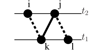
Figure 1: Halo $i$ and $j$ at timestep $t_{2}$ merge and form two halos, $k$ and $l$ at the later timestep $t_{1}$. Halo $k$’s main father is $j$ and the main branch is shown by the solid line.

3.2.1 Identifying anomalous events

Testing to see whether an object is bound is one definitive way of excluding such fake events and it is common practise to sum the kinetic and potential energies of each object and disregard those objects whose total energy is positive (Maciejewski et al., 2009). We combine this technique with an independent anomalous detection method to identify unbound objects at each redshift.

Our prescription for identifying objects participating in anomalous events is as follows. The fathers of an object $k$ at timestep $t_{2}$ are found and if object $k$ has two or more halo fathers that each donate a mass $M_{D}\geq 20M_{p}$, then object $k$ is flagged as a possible fake merger candidate. ($20M_{p}$ is chosen here rather than the mass resolution limit of $40M_{p}$ used in later sections, because $20M_{p}$ is a common mass resolution limit used in other simulation studies and it also maximises the number of possible anomalous events.) The sons of $k$ are then found and if $k$ donates a mass $M_{D}\geq 20M_{p}$ to two or more halos, then it has fragmented and it is identified as an anomalous event candidate. In the case of AHOP halos in this study, which average over their environment and whose substructure is not resolved, this is the sole anomalous event criterion and the same criterion is then imposed on the next halo at timestep $t_{2}$.

For subhalos an additional condition is imposed. Imagine that two halos at timestep $t_{3}$ merge to form a halo, $k$, which hosts a subhalo at the subsequent timestep $t_{2}$. Halo $k$ and its subhalo are then detected as separate halos at the following timestep $t_{1}$ ($t_{1}>t_{2}>t_{3}$). This system has transitioned over three timesteps from two halos, to a halo and a subhalo and back to two halos again, and is hence an anomalous event as no merger has taken place. The subhalos of a given host halo are therefore also examined if the host does not fragment. If a subhalo at $t_{2}$ donates a mass $M_{D}\geq 20M_{p}$ to a halo at $t_{1}$ that is a different halo to the halo son of its host, then it is identified as part of an anomalous event, as are its subhalos (if it has any) and its host. The key ideas of this anomalous event detection method are therefore:

• searching for channels that receive/donate at least $20M_{p}$ from/to two or more different halos and

• ensuring that the host and all associated substructures are flagged in the case of any one of these objects being classified as participating in an anomalous event.

3.2.2 Identifying unbound objects

Table 1 assesses the relative importance of unbound MSM objects above the mass threshold in the simulation ($M\geq 40M_{p}$) for each of the redshifts shown in column $1$ (these redshifts have been chosen because the number of subhalos increases with decreasing redshift in the simulation, as clusters form). The percentages in Table 1 express the number of objects above the threshold mass satisfying the condition in each column as a fraction of the total number of objects above the threshold mass at the redshift in question, with the exception of the bracketed values in column $3$, which show the fraction of anomalous events that are unbound.

There is a positive correlation between the independently identified anomalous events and unbound objects, with a large fraction of the anomalous events being unbound (henceforth unbound refers either to an object with total energy $E_{T}\geq 0$ or an object participating in an anomalous event or both). Not all objects in column $3$ have $E_{T}\geq 0$, however, and so there is a small population of unbound objects at each redshift that would be missed if just a requirement of $E_{T}\geq 0$ were imposed on every object.

Table 1: The relative importance of unbound MSM halos and subhalos above the threshold mass ($M\geq 40M_{p}$) in the $512^{3}$ simulation.

Redshift	$E_{T}\geq 0$	Anomalous ($E_{T}\geq 0$)	Objects with
	$\%$	$\%$	recorded accretion
			$\%$
$0.49$	23.1	7.85 (84.8)	73.5
$0.23$	23.7	8.57 (87.3)	73.2
$0.01$	24.1	9.14 (89.7)	73.4

Only bound objects above the mass threshold can have a recorded accretion value in this study, despite $\sim 38\%$ of all the objects at each of the redshifts shown in Table 1 having a mass below the chosen threshold limit. Bound objects below threshold, however, are not removed from the sample and so it is possible for a bound object with $M<40M_{p}$ to be a main father. We therefore avoid biasing the accretion events in the simulation, whilst ensuring that only well resolved objects have an accretion value.

Column $4$ shows the fraction of objects above the mass threshold with a recorded accretion value. A very small fraction of bound objects with $M\geq 40M_{p}$ do not have a measured accretion rate because they do not satisfy some additional criteria imposed by the accretion algorithm, which we explain in the following section.

3.3 The accretion algorithm

In detecting substructure, Springel et al. (2001) required that several of the most bound particles of the main father were included in the main son $-$ this was more robust than tracking the evolution of the single most bound particle, which essentially performs a random walk across time. We have defined the main son as the son which receives the most mass from the object of interest, consistent with our main father definition.

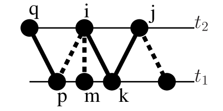
Figure 2: A schematic illustrating the halosub accretion algorithm that accounts for accretion onto halos and subhalos. In this example object $k$, whose main father is object $j$ (solid line), has been identified as the main son of object $i$ (solid line). The accretion onto $k$ using the halosub method is therefore $(1-f_{j})M_{k}$, where $f_{j}$ is the fraction of $k$’s mass that comes from $j$. Object $m$ is not the main son of object $i$ and because it doesn’t have any other fathers it is skipped. Object $p$’s main father is $q$, hence the accretion onto $p$ is $(1-f_{q})M_{p}$. The halosub method therefore only ever records zero or positive accretion rates.

We shall henceforth refer to the algorithm that computes accretion onto halos and associated substructures as the “halosub” method and it is illustrated in Fig.2. For object $i$ at timestep $t_{2}$ the main son $k$ (solid line) is identified. Using our main son definition this means that most of $i$’s mass goes to $k$ and the remainder goes to $m$ and $p$. The father that contributes the most mass to $k$ is then found; in this example $j$ is the main father (solid line). The mass accretion onto $k$ is therefore $(1-f_{j})M_{k}$ where $f_{j}$ is the fraction of $k$’s mass that comes from object $j$. Object $k$ is now flagged and the accretion onto the other sons of $i$, $m$ and $p$, is considered. Since $m$ is not the main son of $i$ and $m$ doesn’t have any other fathers, an accretion value for $m$ is not recorded and it is flagged as an orphan. If however one of the sons, $p$, of the object of interest does experience mass accretion, we identify the main father, $q$, and record the mass accreted: $(1-f_{q})M_{p}$. Object $p$ would then also be flagged. To summarise, we list the principal features of the halosub method:

• the measured mass accretion onto an object represents the sum of diffuse accretion (material not bound to any resolved structure) and merger-driven growth

• mass loss events are considered to be zero accretion events: measured accretion signals in this study are never negative

• all objects with a recorded accretion value are bound and have a mass $M\geq 40M_{p}$

• no distinction is made between halos and different levels of substructure

Since we do not attempt to measure the mass lost from an object during a given time interval, the accretion rate in this study can be thought of as an upper limit. Note that objects which only lose mass and have a recorded accretion rate of zero are identified as systems where the bound main son of the object of interest has only one bound father. A flagged object means that either the accretion onto that object has already been accounted for or that object has been identified as an orphan.

3.4 Limitations

Other than finite mass and time resolutions which are shortcomings of any simulation, we consider the growth of halos and subhalos in a $\Lambda$CDM universe without a prescription for the gas physics. The dark-matter-only simulation satisfies the objective of this study, however: to determine whether halo and subhalo accretion is dependent on environment. The accretion algorithm excludes tidal stripping from the measured accretion rate but objects are stripped of mass in the simulation as they undergo mergers and this reduces their mass.

4 Results

Throughout this section:

1. “object” refers to halos and/or subhalos.

2. the mass of an object corresponds to the total mass, $M_{T}$, detected by the halo-finder.

3. only bound objects above the mass threshold, $M\geq 40M_{p}$, can have a recorded accretion value.

4. the measured mass accretion is the sum of diffuse- and merger-driven accretion: we have not measured mass loss.

5. $\mu\equiv\dot{M}/M$ denotes the specific accretion rate, with units of Gyr^-1, onto an object of mass $M$.

6. $\delta\equiv\delta M_{H}/M_{H}$, where $M_{H}$ represents the mass of a halo.

4.1 Accretion onto dark matter halos

4.1.1 Comparison with EPS

Fig.3 shows the average accretion rate onto the AHOP halos from the simulation as a function of redshift and halo mass. Halos with recorded accretion values are binned in mass at each redshift and the average accretion rate for each mass bin is computed. Averages of the corresponding mass bins over redshift then yield constant $\left<M_{H}\right>$ values (W02 adopt an alternative technique, however, by binning the $z=0$ halos in mass and then averaging over all the accretion trajectories in each bin at each redshift). The solid lines show the accretion rates onto the AHOP halos using the halosub method, and the error bars indicate the $1\sigma$ errors on the mean accretion rate. The EPS predictions for each of the $\left<M_{H}\right>$ bins, computed using equation (1), are shown as the dashed lines.

Figure 3: The average halo accretion rate as a function of redshift and halo mass. The accretion values onto the AHOP halos are shown as the solid lines for each of the five $\left<M_{H}\right>$ bins, with the errors corresponding to the $1\sigma$ errors on the mean accretion rate. The EPS curves using equation (1) are shown as the dashed lines for each mass bin.

Fig.3 shows that the simulation mass trajectories have a lower gradient across redshift than the EPS curves, which overestimate the accretion rate onto the lowest mass halos in the simulation at high redshift by a factor of $\sim 2$, and underestimate it by a factor of $\sim 1.6-1.8$ at $z=0$. It is tempting to think that the enhanced accretion onto halos with respect to EPS theory at low redshift results from the exclusion of mass loss in our measured halo accretion rate. However, EPS doesn’t account for mass loss from halos either: halos only grow with time by construction. The offset with EPS should therefore be regarded as an offset in gradient and Fig.3 implies that the Lacey & Cole (1993) EPS formalism may only require minor adjustment to reproduce the simulated trajectories.

4.1.2 The different accretion modes

Figure 4: The total mass accretion rate onto the AHOP halos per comoving cubic Mpc as a function of redshift, halo mass and $\delta$ ($\equiv\delta M_{H}/M_{H}$). The mass bins correspond to the $\left<M_{H}\right>$ bins in Fig.3, with the lower mass curves shifting to higher $z$. The dashed and thin solid lines show each halo mass bin decomposed into halos with $\delta\leq 0.02$ (minor-merger $\&$ diffuse accretion) and $\delta\geq 0.08$ (major-merger $\&$ diffuse accretion) respectively. The thick solid lines show the mass trajectories integrated over all $\delta$.

Figure 5: The total mass accretion rate onto the AHOP halos per comoving cubic Mpc as a function of halo mass and accretion mode (denoted by $\delta$), shown for several redshifts. The linestyles have the same meaning as in Fig.4 except we also include halos with $0.02<\delta<0.08$ shown by the dotted lines.

The mass accreted onto the AHOP halos in Fig.3 is the summed contribution of diffuse accretion events and minor and major-merger events, hence in Fig.4 we examine the relative importance of these accretion modes as a function of halo mass and redshift. At each redshift, the dimensionless quantity $\delta$ ($\equiv\delta M_{H}/M_{H}$) was computed for each accretion event: the dashed lines and the thin solid lines show halos with $\delta\leq 0.02$ (minor-mergers $\&$ diffuse accretion) and $\delta\geq 0.08$ (major-mergers $\&$ diffuse accretion) respectively. The total mass accretion rate per comoving cubic Mpc for halos in a given mass bin and of a given $\delta$ at each redshift was then computed. The thick solid lines show the total mass accretion rate per comoving cubic Mpc integrated over all $\delta$. For a given linestyle, the lower mass curves shift to higher redshifts.

At high redshift, all halos are found to accrete mass diffusely in high fractional events with the peak in activity shifting to lower redshifts for more massive halos. As the mass accreted onto the lowest mass halos via minor-mergers and diffuse accretion starts to plateau at low redshift, minor-merger and diffuse accretion activity onto the more massive halos starts to rapidly accelerate: low mass halos and non-halo material are being accreted onto larger structures. By $z=0$, the combined minor-merger and diffuse accretion signals dominate the growth of all halos. We further remark that the dashed curves have a similar cosmological evolution to the “radio-mode” integrated black hole accretion rate density curves found by C06 and Bower et al. (2006), but leave a more detailed discussion for Section 5.4.

We have tested the ability of the cut-in-delta method at distinguishing between merger type by adopting the more classical progenitor mass ratio. Each progenitor $j$ of accretor $k$ was assumed to merge in turn with $k$’s main father $i$, with progenitor mass ratio $\chi\equiv M_{i}/M_{j}$, donating $f_{j}M$ to accretor $k$ at the following timestep, where $f_{j}$ denotes the fraction of $k$’s mass that comes from $j$. Events with $\chi\leq 3$ ($\chi>3$) were recorded as major (minor) mergers. We found that major mergers and diffuse accretion events with $\delta\geq 0.08$ had a very similar cosmological evolution to the $\delta\geq 0.08$ curves in Fig.4. The minor merger and diffuse accretion events with $\delta\leq 0.02$ also showed a similar behaviour to the $\delta\leq 0.02$ curves in Fig.4, except there were more minor mergers at higher redshift for all mass curves. These features do not affect our conclusions in Section 5.4, however.

Fig.5 shows the shift from major-merger and diffuse- dominated growth at high redshift to minor-merger and diffuse- dominated growth at low redshift, more clearly. The linestyles have the same meaning as in Fig.4, except we also include the halos with $0.02<\delta<0.08$, shown by the dotted lines. It can be seen that minor-mergers and diffuse accretion events start to significantly contribute to growth for $z<0.5$, and by $z=0$ drive accretion onto all halo masses.

Qualitatively we find very similar results to Figs. 4 and 5 when halos are binned in $\mu$ ($\equiv\dot{M}/M$) instead of $\delta$, but the thin major-merger curves in Figs. 4 and 5 decouple from the thick curves at later epochs, for all masses. This is probably because in transitioning from $\delta$ to $\mu$, one must divide $\delta$ by the time interval during which mass is accreted, and at higher redshifts this time interval is smaller (time is not a linear function of redshift) and $\mu$ is hence larger than it is for a given $\delta$ onto a halo of fixed mass at lower redshift.

Figure 6: The mean specific accretion rate onto halos and subhalos using the halosub method, plotted as a function of object mass for three redshifts corresponding to $z=0.49$ (triple-dot-dashed lines), $z=0.23$ (dashed lines) and $z=0.01$ (solid lines). Lines of a given linestyle from bottom to top represent the accretion onto the AHOP halos and the MSM halos and subhalos respectively. The thick line shows the W02 result, obtained by using equation (3) and equation (5) at $z=0.01$.

Figure 7: The mean specific accretion rate as a function of mass shown for $z=0.49$ (triple-dot-dashed lines), $z=0.23$ (dashed lines) and $z=0.01$ (solid lines) using the halosub accretion method. For a given linestyle, the bottom line shows the MSM halos, the middle line shows the MSM halos and subhalos and the top line shows the MSM subhalos.

4.2 Accretion onto subhalos

In this section, the AHOP halos are resolved into constituent MSM halos and subhalos and the halosub method is applied to these resolved structures to account for accretion onto objects in groups and clusters. We begin by comparing the AHOP halo and MSM halo and subhalo specific accretion rates with the results found in the W02 simulation study. The mass of a halo or subhalo is henceforth denoted by $M$, in contrast with the previous section which only recorded accretion onto halos with mass $M_{H}$.

4.2.1 Comparing the halosub accretion algorithm with W02

Fig.6 plots the average specific accretion rate for all bound objects from the simulation as a function of average object mass for redshifts corresponding to $z=0.49$ (triple-dot-dashed lines), $z=0.23$ (dashed lines) and $z=0.01$ (solid lines). These redshifts have been chosen because the epoch of cluster formation is $z<1$. The lines of a given linestyle from bottom to top represent the accretion onto the AHOP halos and MSM halos and subhalos respectively. The thick line shows the W02 result at $z=0.01$ using equation (3) (strictly, equation (3) holds at $z=0$ but we cannot use our anomalous detection method at this redshift). The W02 result was calculated by binning in mass each $z=0.01$ bound AHOP halo accretor and computing the corresponding average W02 $\alpha$ parameter in equation (5) for each mass bin ($\alpha$ is inversely proportional to halo formation redshift).

The specific accretion rate onto the MSM objects is systematically larger than the AHOP specific accretion rates at every mass when considering a given redshift. The MSM method resolves the substructure that has been averaged out in the AHOP halo, so the main MSM host halo and subhalos are individually less massive than the AHOP counterpart. The offset with MSM is probably caused by dividing by the larger AHOP mass, and this offset increases with increasing mass because at larger masses subhalos occupy a larger fraction of the total AHOP mass. The mass difference between AHOP and the main host MSM halo therefore increases with increasing AHOP mass (and there are more detected halos than subhalos at a given redshift in the simulation, so the halos dominate the MSM halo and subhalo accretion signal).

W02 fitted the accretion trajectories of their $z=0$ halos averaged over environment in a WMAP1 cosmology and so their result can be directly tested against the AHOP curve at $z=0.01$ which also averaged over environment, but in a universe with a WMAP3 cosmology (W02 argue that their fitting formula does not depend on the chosen cosmology). We find that the W02 specific accretion rate has a stronger mass dependence than found for the AHOP halos in this study and so for the large galaxy- and group- sized dark halos, overpredicts the specific accretion rate by a factor of $\sim 1.5$.

Recent studies have shown that some halo-finding algorithms can lead to large uncertainties in the halo accretion rate (Genel et al., 2009; Hopkins et al., 2010). The disagreement across mass with W02 in Fig.6, however, does not result from differences in halo-finder: the AHOP algorithm is very similar to the modified bound density maxima technique of Bullock et al. (2001) used in W02. The disagreement most likely arises because W02 impose different criteria to identify the main son and main father. They adopt a policy, in some cases, of tracking the single most bound particle, which is misleading as the trajectory essentially performs a random walk across time. By constrast, we rigorously identify false merger candidates and adopt an accretion algorithm that tracks channels which donate/receive the most mass (and recall that by allowing a bound object below the mass threshold to be a main father, we do not bias the accretion events). Our method hence avoids using ad-hoc criteria.

Figure 8: The two-point correlation function plotted as a function of the mean inter-object separation (in physical coordinates) for four redshifts corresponding to $z=2.03,0.49,0.23$ and $z=0.01$. The lines in each panel represent the bound MSM halo-halo (solid), halo-subhalo (dotted) and subhalo-subhalo (short-dashed) accretors. The vertical long-dashed lines represent an estimate of the resolution limit in $r$ at each redshift.

Figure 9: Distributions of $\Delta v/v_{c}$ for the halo (thick lines) and subhalo (thin lines) accretors, where $\Delta v$ represents the relative velocity between an accretor’s main father and one of its other progenitors, and $v_{c}$ is the accretor’s circular velocity. The halo and subhalo accretors are divided into different mass bins, shown by the ranges of $M_{H}$ and $M_{S}$ respectively, and correspond to the same objects shown in Fig.7.

4.2.2 Accretion onto MSM halos and subhalos

Fig.7 shows the specific accretion rate from bottom to top of MSM halos, MSM halos and subhalos, and MSM subhalos with the linestyles having the same meaning as in Fig.6. The average specific accretion rates onto halos ($\mu_{H}$) and subhalos ($\mu_{S}$) have weak mass dependencies for each of the redshifts shown: $\langle\mu_{H}\rangle\propto M^{0.2}$ and $\langle\mu_{S}\rangle\propto M^{0.1}$ at $z=0.01$, for example. Each of the halo, halo and subhalo, and subhalo curves shift downwards with decreasing redshift: the average specific accretion rate onto a subhalo at $z=0.49$ is a factor of $1.3-1.4$ greater than at $z=0.01$, for example. Major merger and diffuse accretion events at higher redshifts, when the universe was more dense, are more prominent.

Fig.7 also reveals that the subhalo accretors (and this includes the subhalos with a zero accretion rate) accrete at a larger rate, on average, than the halo accretors for $z<0.5$ at the mass scales shown. This, however, only causes a modest shift from the halo curve to the halo and subhalo curve at each redshift, because there are more halo accretors than subhalo accretors in the simulation, indicating that the subhalos are not responsible for the AHOP to MSM shift in accretion at each redshift in Fig.6. The enhanced accretion onto subhalos can be understood by examining their mutual clustering and the relative velocity of their progenitors compared to their internal velocity, and both of these processes are discussed in the following sections.

4.2.3 The clustering of halos and subhalos

The main aim of this study is to investigate whether there is a relationship between the rate at which objects accrete mass and their environment and so in this section the clustering properties of halos and subhalos at different redshifts are examined. In the following section we specifically target accretors in different cluster-scale environments.

Fig.8 shows the two-point correlation function, $\xi$, for the MSM accretors from the simulation as a function of the physical separation distance $r$, at the same three redshifts shown in Figs. 6 and 7 and at a much higher redshift of $\sim 2$. The Landy & Szalay (1993) $\hat{w}_{4}$ estimator was used to compute $\xi$, requiring random catalogues for each redshift. Our catalogues sampled $300000$ objects at each redshift and were hence larger than the corresponding total number of detected halos and subhalos ($z=2.03:156120;z=0.49:211537;z=0.23:216232;z=0:223781$). For each panel in Fig.8, the solid lines represent the halo-halo pairs, the dotted lines represent the halo-subhalo pairs and the dashed lines represent the subhalo-subhalo pairs. Only the clustering of bound accretors was measured: halo-subhalo pairs correspond to the clustering of all bound halo accretors with all bound subhalo accretors, for example. The vertical dashed lines show the average total diameter of an object at the redshift in question and represent an estimate of the resolution limit in $r$.

Fig.8 demonstrates that subhalo-subhalo pairings are a factor of $\sim 2$ more clustered than halo-halo pairings at large physical scales at low redshift. This factor increases to $\sim 10-15$ at lower separation scales: subhalos, by definition, reside within halos and so cluster more strongly at small scales. The drop-off in clustering amplitude at the lowest scales should be ignored as this occurs at scales that are below the estimated resolution limit.

The subhalo-subhalo correlation function is the sum of two terms: the first describes the clustering of subhalos within the same host and the second describes the clustering of subhalos that belong to different hosts. For small separations, the subhalo-subhalo correlation function has a strong contribution from pairs of subhalos in the same host. The clustering of halo-halo pairings is lower at these scales because these scales approach the size of halos, and so it is less common to find two halos close to each other without one or both member(s) of the pair being a subhalo. At larger scales, subhalos belonging to different hosts contribute strongly to the subhalo-subhalo clustering strength.

The clustering amplitudes of the three curves also evolve with redshift: the correlation length of the subhalo-subhalo curve increases by a factor $\sim 3$ towards $z=0$, for example. This is probably because at lower redshift there are more dense clusters and more subhalos within a given host in the simulation, hence there is a stronger contribution to the subhalo-subhalo clustering amplitude than at higher redshift at the separation scales shown.

4.2.4 Measuring the relative velocities between the accretors’ progenitors

Having established that subhalos at sub-cluster scales are more clustered than halos, especially at small scales, we now examine the distributions of $\Delta v/v_{c}$, where $\Delta v$ represents the relative velocity between an accretor’s main father and one of its other progenitors, and $v_{c}$ is the accretor’s circular velocity. If $\Delta v/v_{c}$ tends to be smaller, on average, for subhalo accretors than halo accretors for example, then accretion onto halos will tend to be more suppressed than accretion onto subhalos. Fig.9 shows the distributions of this ratio for halos (thick lines) and subhalos (thin lines) at the same redshifts shown in Fig.7. The $\Delta v/v_{c}$ ratio was computed for each progenitor $k$ (not equal to the main father $j$) of a given accretor: each particle accreted from the background was counted as an individual relative velocity event, as was each halo/subhalo progenitor. So if, for example, an accretor has a main father $j$, a father $k$, and also accretes two particles from the background, $m$ and $n$, then three separate relative velocities with respect to $j$ are computed for that accretor. The accretors were binned in mass, and the different halo and subhalo mass bins are shown by the ranges of $M_{H}$ and $M_{S}$ in Fig.9, respectively.

It can be seen from Fig.9 that the distributions of $\Delta v/v_{c}$ for the halo and subhalo accretors are similar: they depend quite weakly on mass and their peaks coincide.

4.2.5 Revisiting the enhanced accretion onto subhalos in Fig.7

It is well established that in simulations, after infall, subhalos experience mass loss via tidal stripping, tidal heating and disk shocking (Gnedin et al., 1999; Dekel et al., 2003; Taylor & Babul, 2004; D’Onghia et al., 2010), and have a large velocity dispersion that scales with their host’s mass. Mass stripping from an object in this dark-matter-only study is recorded as zero accretion, and so one would perhaps expect subhalos to be accreting at low rates, on average. We have found, however, that most of the subhalo accretors in the simulation at $z<0.5$ reside in the outer regions of their host, with $\sim 70\%$ located beyond their host’s virial radius. (The halo virial radius roughly corresponds to $r_{200}$, which encloses the region within which the halo density is at least $200$ times the critical density of the universe.) Most of these subhalos have therefore probably not been significantly stripped of their mass. Infact, we find the opposite trend in Fig.7: subhalos of a given mass in the simulation have a larger rate of accretion, on average, than halos of the same mass. Having demonstrated that there is no significant difference between the halo and subhalo accretor distributions of $\Delta v/v_{c}$, we conclude that the enhanced subhalo accretion rates are driven by the very frequent interactions between subhalos of the same host at small scales (Fig.8). Halos are less clustered at small scales and so accrete at lower rates, on average.

Figure 10: $\langle\mu\rangle$ plotted as a function of object mass ($M$) and environment mass ($M_{E}$) for MSM-detected objects. The lines in row one, from bottom to top, represent $M_{E}<10^{11.5}M_{\odot}$, $10^{11.5}M_{\odot}\leq M_{E}<10^{12.5}M_{\odot}$, $10^{12.5}M_{\odot}\leq M_{E}<10^{13.5}M_{\odot}$ (solid lines) and $10^{13.5}M_{\odot}\leq M_{E}<10^{14.5}M_{\odot}$ (triple-dot-dashed lines) using a sphere radius ($R$) of $1.46h^{-1}$Mpc. The second row shows the results for a sphere radius of $3.65h^{-1}$Mpc for environment mass bins $M_{E}<10^{12.5}M_{\odot}$, $10^{12.5}M_{\odot}\leq M_{E}<10^{13.5}M_{\odot}$ (solid lines) and $10^{13.5}\leq M_{E}<10^{14.5}M_{\odot}$ (triple-dot-dashed lines). The vertical arrow indicates the direction of increasing environment mass for both rows, with the exception of the highest environment mass bins in row one, which mostly lie beneath the second highest environment bins. The open squares joined by solid lines illustrate the EPS result using equation (1) and the open stars show accretion onto the MSM halos and subhalos, independent of their environment. Columns one, two and three correspond to $z=0.49,z=0.23$ and $z=0.01$.

Figure 11: The two-point correlation function plotted as a function of the mean inter-object separation (in physical coordinates) for the four redshifts corresponding to $z=2.03,0.49,0.23$ and $z=0.01$. The $z=2.03$ panel shows the MSM objects whose masses satisfy $10^{10.6}M_{\odot}\leq M<10^{10.9}M_{\odot}$ with $\mu<0.35$Gyr^-1 (solid), $0.35$Gyr${}^{-1}\leq\mu<0.6$Gyr^-1 (dotted) and $\mu\geq 0.6$Gyr^-1 (short-dashed). The lower redshift panels show the MSM objects whose masses satisfy $10^{11}M_{\odot}\leq M<10^{11.3}M_{\odot}$ with $\mu<0.1$Gyr^-1 (solid), $0.1$Gyr${}^{-1}\leq\mu<0.2$Gyr^-1 (dotted) and $\mu\geq 0.2$Gyr^-1 (short-dashed). The vertical long-dashed lines represent an estimate of the resolution limit in the separation scale at each redshift.

4.3 Halo and Subhalo environment

In this section we specifically target the effect an object’s environment at cluster scales has on the rate at which it accretes mass. There are two popular, independent measures of environment in the literature; the overdensity $\delta_{R}(\textbf{x})$ in a sphere of radius $R$ (Lemson & Kauffmann, 1999; Wang et al., 2007) and halo bias (Sheth & Tormen, 2004; Gao & White, 2007). We adopt two similar measures of an object’s environment: the first defines an environment mass within a cluster-sized sphere and the second uses the two-point correlation function.

4.3.1 Environment mass

We have defined the environment of a halo and a subhalo as the total mass, $M_{E}$, contained within a sphere of radius $R$ centred on the object of interest. $M_{E}$ includes the mass of all those objects whose centres lie within the sphere as well as the mass of the object the sphere is centred on. We consider spheres of radii $R=1.46h^{-1}$Mpc and $R=3.65h^{-1}$Mpc because a) these scales represent both typical clusters and much larger clusters and b) various authors have found that the dependence of some halo properties on environment, such as halo formation redshift, are sensitive to the choice of sphere radius (Lemson & Kauffmann, 1999; Harker et al., 2006; Hahn et al., 2009). Both of these environment mass definitions are applied to each bound accretor at the redshift under consideration, with only bound accretors having a recorded $M_{E}$ value. Unbound objects and resolved objects with $M\leq 40M_{p}$ are not, however, excluded from the sample as these objects could be part of a bound object’s environment.

The first row of Fig.10 plots the specific accretion rate onto halos and subhalos as a function of average object mass ($M$) and average environment mass ($M_{E}$) for $z=0.49$ (first column), $z=0.23$ (second column) and $z=0.01$ (third column) using a sphere radius of $1.46h^{-1}$Mpc. The second row of Fig.10 shows the results using a larger sphere radius of $3.65h^{-1}$Mpc at the same three redshifts.

The solid lines represent the environment mass bins which from bottom to top for the first row are: $M_{E}<10^{11.5}M_{\odot}$, $10^{11.5}M_{\odot}\leq M_{E}<10^{12.5}M_{\odot}$ and $10^{12.5}M_{\odot}\leq M_{E}<10^{13.5}M_{\odot}$. The triple-dot-dashed line shows the largest environment mass bin of $10^{13.5}M_{\odot}\leq M_{E}<10^{14.5}M_{\odot}$. For the larger scale environments in the second row (from bottom to top): $M_{E}<10^{12.5}M_{\odot}$, $10^{12.5}M_{\odot}\leq M_{E}<10^{13.5}M_{\odot}$ (solid lines) and $10^{13.5}M_{\odot}\leq M_{E}<10^{14.5}M_{\odot}$ (triple-dot-dashed lines). The vertical arrow shows the direction of increasing environment for all panels, with the exception of the largest environment mass bins in the first row, which mostly lie beneath the second largest environment bins. The stars in each panel represent the accretion onto MSM halos and subhalos independent of their environment and the squares joined by solid lines show the EPS results.

The relationships found in the previous sections are preserved in Fig.10: the specific accretion rate increases with object mass for objects in most environments and decreases towards $z=0$ (as was shown in Fig.7), and EPS consistently underestimates the mass accreted onto all object masses (as was shown for halos at $z<1$ in Fig.3). The most striking feature of Fig.10, however, is that objects of a given mass residing in more massive environments do not accrete at a particularly enhanced rate compared with objects of the same mass in much lower mass environments. This suggests that the specific accretion rate onto halos and subhalos does not depend strongly on environment at cluster scales. Objects in cluster mass environments shown in the first row (triple-dot-dashed lines) mostly accrete less mass than in lower mass environments, but the number of objects in cluster mass surroundings is limited by the choice of sphere radius. This effect is not seen for the larger-scale environments shown in the second row, for example, where merging between subhalos on the outskirts of the host halo is probably driving accretion (but only at a slightly higher overall rate). The second row shows that the specific accretion rate only depends weakly on environment at larger scales that probe the outermost regions of clusters. This weak environment dependence in rows $1$ and $2$ therefore seems to suggest that the increased interaction rates of halos in group- and cluster- mass environments are not sufficiently large enough to significantly overcome the large halo relative velocities, resulting in only a modest net increase in accretion.

Halos dominate the accretion signals in Fig.10, but we find the same trends at each of the chosen redshifts when just subhalos are plotted as a function of their mass and environment mass. There are two differences, however: the subhalos a) accrete at higher rates and b) reside only in larger mass environments. The subhalo curves have been omitted in Fig.10 for clarity.

Other authors have quantified environment by computing the overdensity $\delta_{R}$ in a sphere of radius $R$, rather than the mass (Lemson & Kauffmann, 1999; Harker et al., 2006; Hahn et al., 2009; Fakhouri & Ma, 2009, 2010). We therefore calculated a weighted environment density for each halo and subhalo accretor by using the standard SPH cubic spline window function (Monaghan & Lattanzio, 1985) which weights the mass contributions from objects close to the centre of the sphere more strongly than those further away. Fakhouri & Ma (2009) showed that for halos more massive than $10^{14}M_{\odot}$, the density of the object the sphere is centred on starts to dominate the contributions to $\delta_{R}$, and so the central object’s contribution was therefore both included and excluded in two separate weighted environment density measures. When binned in environment density, the same weak environment dependence as in Fig.10 was found in both cases.

4.3.2 Clustering in different accretion schemes

In this section we use the correlation function as an alternative means to Section 4.3.1 of measuring an object’s environment, except we do not restrict our analysis to just cluster scales of a few Mpc. We consider samples of objects with very similar masses at different redshifts and examine whether objects of a given mass which accrete at larger rates have a larger clustering amplitude. This also tests the work by Percival et al. (2003), who found that at $z=2$ halos of a given mass accreting at different rates do not cluster differently.

The $z=2.03$ panel in Fig.11 shows the correlation function for all those objects whose mass satisfies $10^{10.6}M_{\odot}\leq M<10^{10.9}M_{\odot}$ with $\mu<0.35$Gyr^-1 (solid), $0.35$Gyr${}^{-1}\leq\mu<0.6$Gyr^-1 (dotted) and $\mu\geq 0.6$Gyr^-1 (dashed). The lower redshift panels show the correlation function for objects whose mass satisfies $10^{11}M_{\odot}\leq M<10^{11.3}M_{\odot}$ with $\mu<0.1$Gyr^-1 (solid), $0.1$Gyr${}^{-1}\leq\mu<0.2$Gyr^-1 (dotted) and $\mu\geq 0.2$Gyr^-1 (dashed). The mass interval for $z<0.5$ has been chosen because it lies below the break mass, $M_{\star}$, in the mass function at these redshifts and so we do not bias $\mu$. For comparison, the mass interval in the $z\sim 2$ panel lies closer to $M_{\star}$. The vertical dashed lines represent an estimate of the resolution limit in the separation scale (same as the vertical dashed lines in Fig.8).

At well resolved non-linear small scales for $z<0.5$, objects with high specific accretion rates are up to a factor of $\sim 3$ more clustered than the lower accreting objects, whereas at larger linear scales the difference in clustering between different accretors is much smaller. For the cluster-scale environments of the first row of Fig.10, corresponding to an $r$ value of $2.92h^{-1}$Mpc, there is a weak environment dependence, with objects of larger $\mu$ being slightly more clustered. Fig.11 therefore provides further evidence that the mass accreted onto halos and subhalos of a given mass weakly depends on their environment at cluster scales.

In contrast to the $z<0.5$ behaviour, there is very little difference in clustering between different accretors with $10^{10.6}M_{\odot}\leq M<10^{10.9}M_{\odot}$ at $z\sim 2$ and this holds for both the linear and non-linear scales shown. We therefore agree with the conclusions of Percival et al. (2003) at $z\sim 2$ but show that they break down at $z<0.5$, where there is a larger difference in clustering between high accretors and low accretors of a given mass at all scales.

5 Discussion

5.1 Disagreement with EPS theory

Despite its success at reproducing the dark halo mass function in simulations, we find that the analytic EPS calculation shows significant departures from the halo accretion rates found in our simulation at both low and high redshift (Fig.3). This simulation study, however, is not the first to report disagreement with EPS theory at high redshift: Cohn & White (2008) examined the accretion onto halos of mass $M_{H}=5-8\times 10^{8}h^{-1}$M_⊙ at $z=10$ and found that EPS overestimated the halo accretion rate by a factor $\sim 1.5$ (using a lookback time of $50$ Myrs). Fig.3 shows a similar behaviour, with EPS overpredicting the accretion rate onto halos of mass $M_{H}\sim 10^{10.7}M_{\odot}$ by a factor of $\sim 2$ at $z=8$. One might expect EPS to overestimate accretion onto halos at high redshift because it assumes that collapse is spherical and that the density barrier is fixed in height (Lacey & Cole, 1993) whereas it has been shown that allowing for ellipsoidal collapse and treating the critical density contrast for collapse as a free parameter better reproduces the N-body halo mass function (Sheth et al., 2001; Sheth & Tormen, 2002). This modification reduces the critical density contrast for collapse by a factor of $\sqrt{0.7}$ (M06) which reduces $f(M_{H})$ in equation (1) by the same factor, causing a slight shift in the dashed curves in Fig.3 but otherwise having no effect on the redshift or mass dependence.

The disagreement might arise because EPS theory is only approximate: (i) it assumes spherical collapse, whereas halos in dark-matter-only simulations are triaxial; (ii) it contains no dynamical information, and so is unable, for example, to account for mass being stripped from one halo and then being accreted onto another; (iii) it cannot account for accretion onto substructures; and (iv) it averages over halo environment. The latter restrictions are particularly problematic in the non-linear regime at $z<1$, when accretion onto structures embedded within clusters is of interest (Fig.10). Recent attempts to incorporate an environment dependence into the EPS excursion set theory (Maulbetsch et al., 2007; Sandvik et al., 2007; Zentner, 2007; Desjacques, 2008) could modify equation (1) which might result in better agreement with our simulation results for $z<1$ in Fig.10. Benson et al. (2005) highlighted further weaknesses with the EPS formalism that could also account for the offset in Figs. 3 and 10. They showed that the Lacey & Cole (1993) EPS formula yields merger rates that are not symmetric under exchange of halo masses, and which do not predict the correct evolution of the Press-Schechter mass distribution, indicating that constructed EPS merger trees are fundamentally flawed.

Despite these limitations, the gradients of the EPS curves in Fig.3 are only slightly steeper than the corresponding simulation curves. This implies that the Lacey & Cole (1993) EPS formalism may only require minor adjustment to agree more closely with the simulation trajectories across mass and redshift.

5.2 The weak relationship between accretion rate and environment at cluster scales

By quantifying accretion onto substructures embedded in groups and clusters, we have moved beyond the limited predictive power of the EPS formalism. Fig.7 demonstrates that subhalos accrete at larger rates than halos of the same mass, on average, in the simulation (by a factor of $\sim 3$ for the lowest mass subhalos at $z=0$). At first glance this appears to contradict recent claims: Angulo et al. (2009) and Hester & Tasitsiomi (2010), for example, have shown that subhalo-subhalo mergers are rare and that subhalos are severely stripped of mass, which probably means that the accretion rates onto their subhalos are likely to be low. The subhalo accretors at low redshift in this study, however, form a subsample of subhalos that are safely above the mass resolution limit and that are mostly located at large distances from their host’s centre, with $\sim 70\%$ residing beyond their host’s virial radius. (The halo virial radius approximately encloses the region within which the halo density is at least $200$ times the critical density of the universe). These subhalos are probably not therefore being significantly stripped of mass, unlike the subhalos in recent studies. The mass-selected nature of our subhalo accretors and the different spatial distribution within their host are therefore the most likely causes of the apparent accretion rate discrepancy with the studies mentioned above. We have further shown that the subhalo accretors in this study are more clustered than the halo accretors at small scales (Fig.8) and that there is no significant difference between the distributions of $\Delta v/v_{c}$, where $\Delta v$ is the relative velocity between an accretor’s main father and one of its other progenitors, and $v_{c}$ is the accretor’s circular velocity. The high subhalo accretion rates are therefore likely to be driven by the very frequent interactions at small scales with other subhalos of the same host.

One might expect the accretion rate onto halos and subhalos to depend strongly on environment at larger, cluster-sized scales given the increased rate of interactions in dense environments, but only a weak dependence is found (Figs. 10 and 11). The subhalo accretors reside in only the most massive environments and probably accrete mostly locally from their nearby subhalo neighbours rather than their host, and so this is a possible explanation for their weak relationship between accretion rate and environment. One likely explanation for halos is that the increased interaction rates of halos in group- and cluster- mass environments are not sufficiently large enough to significantly overcome the large halo relative velocities, resulting in only a modest net increase in accretion at cluster scales.

Fakhouri & Ma (2010) examined the environment dependence of accretion onto high mass halos ($M_{H}>10^{12}M_{\odot}$) from the Millennium simulation and found a weak, negative correlation for galaxy-mass halos. We find a weak but positive dependence for all object masses in Fig.10. Our analysis, which extends theirs by accounting for accretion onto substructures, has a different expression for the mass accretion rate but we have found little difference in the results obtained from using the two expressions for bound objects. The obvious source of the discrepancy is therefore the method used to identify anomalies. Genel et al. (2009) have highlighted some fundamental problems with the ‘stitching’ algorithm used by Fakhouri & Ma (2010) to remove anomalous events, demonstrating that it can lead to a double counting of mergers and to a false counting of anomalous events as mergers. They show that this overestimation of the merger rate is particularly problematic for minor-mergers. Predicting the effects that overestimating the merger-rate has on the accretion rate and how this varies as a function of environment is not trivial, but differences between the anomalous event detection methods could explain the difference in the sign of the trend between accretion rate and environment.

The $z=2.03$ panel in Fig.11 reveals that at higher redshift when halos far outnumber subhalos in the simulation, the rate of accretion onto halos is independent of environment, confirming the Percival et al. (2003) result. The Percival et al. (2003) study examined the difference in clustering at $z=2$ between halos of a given mass accreting at different rates. They considered several mass intervals ranging from $10^{10.3}M_{\odot}\leq M_{H}\leq 10^{10.4}M_{\odot}$ to $10^{13.3}M_{\odot}\leq M_{H}\leq 10^{13.6}M_{\odot}$ and concluded for each mass interval that halo accretion rates do not depend on environment at this redshift. We suggest that this apparent lack of environment dependence arises because the halos in the Percival et al. (2003) study and to a lesser extent the halos considered in the $z\sim 2$ panel in Fig.11, represent some of the most massive objects at $z\sim 2$ and hence have bias factors $b>1$ (Sheth & Tormen, 1999). These structures are located at the highest peaks in the density field and so by computing the clustering amplitude of these objects one is essentially measuring the clustering pattern of the highest density peaks at this redshift. It is therefore unlikely that the highest mass halos experiencing different instantaneous accretion rates differ in their clustering. By contrast, the lower mass halos and subhalos in the $z<1$ panels are less biased and so more closely track the clustering of the underlying mass distribution.

5.3 Comparing dark halo growth with black hole growth

Under the assumption that, on average, black hole growth traces dark halo growth (so-called “pure coeval evolution”), M06 tested the predictions of equation (1) for the evolution of the integrated AGN luminosity density for $z\leq 3$. The coeval evolution model tests the hypothesis that the fractional mass accretion rate onto black holes and onto halos are equal (i.e. $\dot{M}/M$ is the same for both black holes and halos), and is consistent with the tight relation inferred between black hole mass and galaxy bulge mass (Tremaine et al., 2002, but see Batcheldor 2010 for an alternative interpretation), and is easy to test. M06 found the predicted integrated AGN luminosity density to be in remarkable agreement with the bolometric AGN luminosity density measured using hard X-ray data. They also found that for $z>0.5$ average black hole growth is well approximated by pure coeval evolution, but for $z<0.5$ the black hole luminosity density tails off more quickly than dark halo growth, and by $z=0$ is lower by a factor of $\sim 2$. They suggested that this slowdown in black hole accretion could be related to cosmic downsizing (e.g. Barger et al., 2005).

Their predictions for dark halo growth were, however, based on EPS theory. The simulation trajectories in Fig.3 show that EPS underestimates halo accretion for $z<1$, and at $z=0$ is a factor of $\sim 1.5-2$ lower for all halo masses. This implies that present day dark halos could be accreting at fractional rates that are up to $\sim 3-4$ times higher than their associated black holes. However, for $1<z<3$, the simulated dark halo accretion trajectories in Fig.3 are reasonably well approximated by EPS. We therefore suggest the following scenario: for $1<z<3$ black holes grow coevally with their dark hosts but for $z<1$, the epoch of cluster formation, their growth significantly decouples from that of their hosts.

It is still plausible that this decoupling is linked to the inference that high mass black holes preferentially “turn off” at low redshifts, leaving the remaining accretion activity dominated by low mass black holes (Heckman et al., 2004). The cause of such downsizing is often assumed to be connected to the physics of the baryon component. Our study reinforces this assumption: if downsizing were a “whole halo” phenomenon it would be manifest in our dark-matter-only simulation, and its absence in our results confirms that we should seek an explanation in the baryons.

5.4 Is halo accretion via minor-mergers and diffuse accretion the cause of radio-mode feedback?

A number of authors have developed semi-analytic models of galaxy-formation that are tuned to reproduce the galaxy luminosity function at low redshift (e.g. Bower et al. 2006; C06; De Lucia et al. 2006). A key ingredient of these models is a low level of feedback from black hole accretion that arises in all galaxies and which increases in importance towards low redshifts. The feedback mechanism has still not been identified: luminous, high accretion-rate AGN only form a small subset of the galaxy population at low redshift and seem unlikely to provide the required feedback in all galaxies. Bower et al. (2006) required black holes to have relatively high accretion Eddington ratios, which may be inconsistent with observations: it seems that the accretion and an associated outflow need to be hidden from view in a so-called “radio-mode”. C06 have assumed that such a mode could be fuelled by Bondi accretion from the hot gas phase of their model, but the observational evidence for such a mechanism has not been demonstrated either.

The survey of Ho et al. (1997) revealed that a high fraction, over $40\%$ of nearby galaxies rising to $50\%-75\%$ of bulge systems, host low luminosity AGN (LLAGN), with the majority of LLAGN accreting at highly sub-Eddington rates in the range $10^{-5}<L_{bol}/L_{Edd}<10^{-3}$. Ho (2005) argued that these are systems where accretion occurs via a radiatively-inefficient advection-dominated accretion flow (ADAF). The accretion flow puffs up the inner disk and material is advected towards the black hole (Narayan, 2002; Ho, 2002, 2008), with outflow being channelled along kinetic-energy-dominated jets (Collin et al., 2003; Ho, 2005, 2008). This finding leads us to suggest that LLAGN, fuelled by low accretion rate ADAFs, may provide the radio-mode feedback.

In our dark-matter-only study, the integrated minor-merger and diffuse halo accretion rate density curves in Fig.4 increase in importance towards the present day for all halo masses. This qualitatively agrees with the cosmological evolution of the black hole radio-mode integrated accretion signal found for each of the different semi-analytic models (Bower et al. 2006; C06). We suggest that the periods when galaxy halo growth is dominated by low accretion rate minor-mergers and diffuse accretion events, are mirrored by low accretion rates onto their associated black holes, and that those in turn produce the LLAGN that may be the radio-mode required for the feedback models.

The integrated accretion rate density onto black holes residing in galaxy-mass halos that are accreting diffusely and via minor-mergers at $z=0$ is also very similar to the integrated accretion rate density onto black holes residing in similar sized halos found by C06, who argue that radio-mode feedback is more effective in more massive systems. Our estimate for the total black hole accretion rate density tests the hypothesis that for black holes with mass $M_{BH}$ residing in halos with mass $M_{H}$,

$$\sum_{i}\dot{M}_{i,BH}(z=0)\sim\alpha\frac{M_{BH}}{M_{H}}\sum_{i}\dot{M}_{i,H}(z=0)$$ (7)

where $\alpha$ describes the non-linearity in the black hole - dark halo mass relation and the index $i$ sums over all galaxy-mass dark halos and all black holes residing in these halos. Equation (7) assumes that black hole growth positively traces dark halo growth, on average (recent claims by Kormendy & Bender 2011, however, argue that for bulgeless galaxies there is no such correlation between black holes and their dark hosts, but the interpretation of this as meaning that there is no such relation for all galaxies has been clearly refuted by Volonteri et al. 2011. In what follows we do not address the reliability of the assumption in equation (7) but rather test its prediction for black hole growth). Ferrarese (2002) found that $\alpha=1.65$ and that galaxy-mass halos with $M_{H}\sim 10^{12}M_{\odot}$ have a black hole - dark halo mass ratio of $\sim 10^{-5}$. According to Fig.4 these halos with $\delta M_{H}/M_{H}\leq 0.02$ have a total accretion rate density of $\sim 7.6\times 10^{7}M_{\odot}$Gyr^-1Mpc^-3 at $z=0$, which when substituted into equation (7) yields a total black hole accretion rate density of $\sim 10^{-5.9}M_{\odot}$yr^-1Mpc^-3. This is very similar to the integrated accretion rate density of $\sim 10^{-5.8}M_{\odot}$yr^-1Mpc^-3 onto supermassive black holes at $z=0$ reported by C06.

The $\delta$ parameter ($\equiv\delta M_{H}/M_{H}$) is a free parameter in our model, but we have found that adopting the more classical progenitor mass ratio, $\chi$, to distinguish between merger type yields almost identical results to Fig.4. This provides confirmation that our $\delta$ cuts are indeed capable of separating minor- and major- merger channels. The $\delta$ parameter is therefore probably no more unconstrained than $\chi$.

We conclude that the low rates of accretion onto dark halos, driven by minor-mergers and diffuse accretion, may provide an alternative explanation to that proposed by C06 for the radio-mode feedback needed to reproduce the observed galaxy luminosity function. The low redshift feedback phenomenon and its cosmological evolution may be driven by the cosmological evolution of halo minor-mergers and diffuse accretion rather than requiring accretion out of a hot gas phase.

6 Conclusions

Outputs from one of the high resolution dark-matter-only Horizon Project simulations have been used to investigate the environment and redshift dependence of accretion onto both halos and subhalos. We have developed a method that computes the combined merger- and diffuse- driven accretion onto halos and all levels of substructure and find that:

• Halo accretion rates vary less strongly with redshift than predicted by the EPS formalism. This offset in gradient for each halo mass curve implies that perhaps minor adjustment to the EPS formula is required.

• Comparison with an observational study of black hole growth leads us to suggest that dark halos at $z=0$ could be accreting at fractional rates that are up to $3-4$ times higher than their black holes.

• Halo growth is driven by minor-mergers and diffuse accretion at low redshift. These latter accretion modes have both the correct cosmological evolution and inferred integrated black hole accretion rate density at $z=0$ to drive radio-mode feedback, which has been hypothesised in recent semi-analytic galaxy-formation models as the feedback required to reproduce the galaxy luminosity function at low redshift. Radio-mode feedback may therefore be driven by dark halo minor-mergers and diffuse accretion, rather than accretion of hot gas onto black holes, as has been recently argued.

• The low redshift subhalo accretors in the simulation form a mass-selected subsample safely above the mass resolution limit and mostly reside in the outer regions of their host, with $\sim 70\%$ beyond their host’s virial radius, and are probably not therefore being significantly stripped of mass. These subhalos accrete at higher rates than halos, on average, at low redshifts. We demonstrate that this is due to their enhanced mutual clustering at small scales: there is no significant difference between the halo and subhalo accretor distributions of $\Delta v/v_{c}$, where $\Delta v$ represents the relative velocity between an accretor’s main father and one of its other progenitors, and $v_{c}$ is the accretor’s circular velocity. The very frequent interactions with other subhalos of the same host drive the high subhalo accretion rates.

• Accretion rates onto halos and subhalos depend only weakly on environment at cluster scales. For halos, it appears that the increased interaction rates in group- and cluster- mass environments are not sufficiently large enough to significantly overcome the large halo relative velocities, resulting in only a modest net increase in accretion at cluster scales. The subhalo accretors only reside in the densest environments and they are likely to be accreting mostly from their nearby subhalo neighbours, rather than from their host. We further demonstrate that halos accrete independently of their environment at $z\sim 2$, as has been found by other authors, but show that this behaviour results from examining the clustering of the most massive halos with large bias factors. When less massive halos below $M_{\star}$ at low redshift are considered, a weak dependence between accretion rate and environment at cluster scales arises.

REFERENCES

- Angulo et al. (2009) Angulo R. E., Lacey C. G., Baugh C. M., Frenk C. S., 2009, MNRAS, 399, 983
- Aubert et al. (2004) Aubert D., Pichon C., Colombi S., 2004, MNRAS, 352, 376
- Babić et al. (2007) Babić A., Miller L., Jarvis M. J., Turner T. J., Alexander D. M., Croom S. M., 2007, AAP, 474, 755
- Barger et al. (2005) Barger A. J., Cowie L. L., Mushotzky R. F., Yang Y., Wang W., Steffen A. T., Capak P., 2005, ApJ, 129, 578
- Batcheldor (2010) Batcheldor D., 2010, ApJL, 711, L108
- Bauer et al. (2005) Bauer A. E., Drory N., Hill G. J., Feulner G., 2005, ApJL, 621, L89
- Benson et al. (2005) Benson A. J., Kamionkowski M., Hassani S. H., 2005, MNRAS, 357, 847
- Blumenthal et al. (1984) Blumenthal G. R., Faber S. M., Primack J. R., Rees M. J., 1984, NATURE, 311, 517
- Bond et al. (1991) Bond J. R., Cole S., Efstathiou G., Kaiser N., 1991, ApJ, 379, 440
- Bower et al. (2006) Bower R. G., Benson A. J., Malbon R., Helly J. C. a., 2006, MNRAS, 370, 645
- Brinchmann & Ellis (2000) Brinchmann J., Ellis R. S., 2000, ApJL, 536, L77
- Bullock et al. (2001) Bullock J. S., Kolatt T. S., Sigad Y., Somerville R. S., Kravtsov A. V., Klypin A. A., Primack J. R., Dekel A., 2001, MNRAS, 321, 559
- Bundy et al. (2006) Bundy K., Ellis R. S., Conselice C. J., Taylor J. E., Cooper M. C., Willmer C. N. A., Weiner B. J., Coil A. L., Noeske K. G., Eisenhardt P. R. M., 2006, ApJ, 651, 120
- Cattaneo et al. (2006) Cattaneo A., Dekel A., Devriendt J., Guiderdoni B., Blaizot J., 2006, MNRAS, 370, 1651
- Cohn & White (2008) Cohn J. D., White M., 2008, MNRAS, 385, 2025
- Collin et al. (2003) Collin S., Combes F., Shlosman I., eds, 2003, Active galactic nuclei : from the central engine to host galaxy Vol. 290 of Astronomical Society of the Pacific Conference Series
- Conroy et al. (2006) Conroy C., Wechsler R. H., Kravtsov A. V., 2006, ApJ, 647, 201
- Cowie et al. (2003) Cowie L. L., Barger A. J., Bautz M. W., Brandt W. N., Garmire G. P., 2003, ApJL, 584, L57
- Cowie et al. (1996) Cowie L. L., Songaila A., Hu E. M., Cohen J. G., 1996, ApJ, 112, 839
- Croton et al. (2006) Croton D. J., Springel V., White S. D. M., De Lucia G., Frenk C. S., Gao L., Jenkins A., Kauffmann G., Navarro J. F., Yoshida N., 2006, MNRAS, 365, 11
- Davis et al. (1985) Davis M., Efstathiou G., Frenk C. S., White S. D. M., 1985, ApJ, 292, 371
- De Lucia et al. (2006) De Lucia G., Springel V., White S. D. M., Croton D., Kauffmann G., 2006, MNRAS, 366, 499
- Dekel et al. (2003) Dekel A., Devor J., Hetzroni G., 2003, MNRAS, 341, 326
- Desjacques (2008) Desjacques V., 2008, MNRAS, 388, 638
- Diemand et al. (2004) Diemand J., Moore B., Stadel J., 2004, MNRAS, 352, 535
- D’Onghia et al. (2010) D’Onghia E., Springel V., Hernquist L., Keres D., 2010, ApJ, 709, 1138
- Faber et al. (2007) Faber S. M., Willmer C. N. A., Wolf C., Koo D. C., Weiner B. J., Newman J. A., et al., 2007, ApJ, 665, 265
- Fakhouri & Ma (2009) Fakhouri O., Ma C., 2009, MNRAS, 394, 1825
- Fakhouri & Ma (2010) Fakhouri O., Ma C., 2010, MNRAS, 401, 2245
- Fakhouri et al. (2010) Fakhouri O., Ma C., Boylan-Kolchin M., 2010, MNRAS, pp 857–+
- Fall & Efstathiou (1980) Fall S. M., Efstathiou G., 1980, MNRAS, 193, 189
- Ferrarese (2002) Ferrarese L., 2002, ApJ, 578, 90
- Gao et al. (2004) Gao L., De Lucia G., White S. D. M., Jenkins A., 2004, MNRAS, 352, L1
- Gao et al. (2005) Gao L., Springel V., White S. D. M., 2005, MNRAS, 363, L66
- Gao & White (2007) Gao L., White S. D. M., 2007, MNRAS, 377, L5
- Genel et al. (2009) Genel S., Genzel R., Bouché N., Naab T., Sternberg A., 2009, ApJ, 701, 2002
- Giocoli et al. (2010) Giocoli C., Tormen G., Sheth R. K., van den Bosch F. C., 2010, MNRAS, 404, 502
- Gnedin et al. (1999) Gnedin O. Y., Hernquist L., Ostriker J. P., 1999, ApJ, 514, 109
- Hahn et al. (2009) Hahn O., Porciani C., Dekel A., Carollo C. M., 2009, MNRAS, 398, 1742
- Harker et al. (2006) Harker G., Cole S., Helly J., Frenk C., Jenkins A., 2006, MNRAS, 367, 1039
- Hasinger et al. (2005) Hasinger G., Miyaji T., Schmidt M., 2005, AAP, 441, 417
- Hatton et al. (2003) Hatton S., Devriendt J. E. G., Ninin S., Bouchet F. R., Guiderdoni B., Vibert D., 2003, MNRAS, 343, 75
- Heckman et al. (2004) Heckman T. M., Kauffmann G., Brinchmann J., Charlot S., Tremonti C., White S. D. M., 2004, ApJ, 613, 109
- Hester & Tasitsiomi (2010) Hester J. A., Tasitsiomi A., 2010, ApJ, 715, 342
- Hiotelis & Popolo (2006) Hiotelis N., Popolo A. D., 2006, APSS, 301, 167
- Ho (2002) Ho L. C., 2002, ApJ, 564, 120
- Ho (2005) Ho L. C., 2005, APSS, 300, 219
- Ho (2008) Ho L. C., 2008, ARAA, 46, 475
- Ho et al. (1997) Ho L. C., Filippenko A. V., Sargent W. L. W., 1997, ApJ, 487, 568
- Hopkins et al. (2010) Hopkins P. F., Croton D., Bundy K., Khochfar S., van den Bosch F., Somerville R. S., Wetzel A., Keres D., Hernquist L., Stewart K., Younger J. D., Genel S., Ma C., 2010, ApJ, 724, 915
- Hopkins et al. (2007) Hopkins P. F., Richards G. T., Hernquist L., 2007, ApJ, 654, 731
- Kormendy & Bender (2011) Kormendy J., Bender R., 2011, NATURE, 469, 377
- Kravtsov et al. (1997) Kravtsov A. V., Klypin A. A., Khokhlov A. M., 1997, ApJS, 111, 73
- Lacey & Cole (1993) Lacey C., Cole S., 1993, MNRAS, 262, 627
- Landy & Szalay (1993) Landy S. D., Szalay A. S., 1993, ApJ, 412, 64
- Lemson & Kauffmann (1999) Lemson G., Kauffmann G., 1999, MNRAS, 302, 111
- Maciejewski et al. (2009) Maciejewski M., Colombi S., Springel V., Alard C., Bouchet F. R., 2009, MNRAS, 396, 1329
- Maulbetsch et al. (2007) Maulbetsch C., Avila-Reese V., Colín P., Gottlöber S., Khalatyan A., Steinmetz M., 2007, ApJ, 654, 53
- McBride et al. (2009) McBride J., Fakhouri O., Ma C., 2009, MNRAS, 398, 1858
- Miller et al. (2006) Miller L., Percival W. J., Croom S. M., Babić A., 2006, AAP, 459, 43
- Monaghan & Lattanzio (1985) Monaghan J. J., Lattanzio J. C., 1985, AAP, 149, 135
- Moore et al. (1999) Moore B., Ghigna S., Governato F., Lake G., Quinn T., Stadel J., Tozzi P., 1999, ApJL, 524, L19
- Nagai & Kravtsov (2005) Nagai D., Kravtsov A. V., 2005, ApJ, 618, 557
- Narayan (2002) Narayan R., 2002, in M. Gilfanov, R. Sunyeav, & E. Churazov ed., Lighthouses of the Universe: The Most Luminous Celestial Objects and Their Use for Cosmology Why Do AGN Lighthouses Switch Off?. pp 405–+
- Neistein & Dekel (2008) Neistein E., Dekel A., 2008, MNRAS, 388, 1792
- Panter et al. (2007) Panter B., Jimenez R., Heavens A. F., Charlot S., 2007, MNRAS, 378, 1550
- Percival et al. (2003) Percival W. J., Scott D., Peacock J. A., Dunlop J. S., 2003, MNRAS, 338, L31
- Sandvik et al. (2007) Sandvik H. B., Möller O., Lee J., White S. D. M., 2007, MNRAS, 377, 234
- Schawinski et al. (2009) Schawinski K., Lintott C. J., Thomas D., Kaviraj S., Viti S., Silk J., Maraston C., Sarzi M., Yi S. K., Joo S., Daddi E., Bayet E., Bell T., Zuntz J., 2009, ApJ, 690, 1672
- Schawinski et al. (2007) Schawinski K., Thomas D., Sarzi M., Maraston C., Kaviraj S., Joo S., Yi S. K., Silk J., 2007, MNRAS, 382, 1415
- Sheth et al. (2001) Sheth R. K., Mo H. J., Tormen G., 2001, MNRAS, 323, 1
- Sheth & Tormen (1999) Sheth R. K., Tormen G., 1999, MNRAS, 308, 119
- Sheth & Tormen (2002) Sheth R. K., Tormen G., 2002, MNRAS, 329, 61
- Sheth & Tormen (2004) Sheth R. K., Tormen G., 2004, MNRAS, 350, 1385
- Somerville & Kolatt (1999) Somerville R. S., Kolatt T. S., 1999, MNRAS, 305, 1
- Somerville & Primack (1999) Somerville R. S., Primack J. R., 1999, MNRAS, 310, 1087
- Springel (2005) Springel V., 2005, MNRAS, 364, 1105
- Springel et al. (2001) Springel V., White S. D. M., Tormen G., Kauffmann G., 2001, MNRAS, 328, 726
- Steffen et al. (2003) Steffen A. T., Barger A. J., Cowie L. L., Mushotzky R. F., Yang Y., 2003, ApJL, 596, L23
- Taylor & Babul (2004) Taylor J. E., Babul A., 2004, MNRAS, 348, 811
- Tormen (1997) Tormen G., 1997, MNRAS, 290, 411
- Tormen et al. (1998) Tormen G., Diaferio A., Syer D., 1998, MNRAS, 299, 728
- Tremaine et al. (2002) Tremaine S., Gebhardt K., Bender R., Bower G., Dressler A., Faber S. M., Filippenko A. V., Green R., Grillmair C., Ho L. C., Kormendy J., Lauer T. R., Magorrian J., Pinkney J., Richstone D., 2002, ApJ, 574, 740
- Tweed et al. (2009) Tweed D., Devriendt J., Blaizot J., Colombi S., Slyz A., 2009, AAP, 506, 647
- Vale & Ostriker (2006) Vale A., Ostriker J. P., 2006, MNRAS, 371, 1173
- van den Bosch (2002) van den Bosch F. C., 2002, MNRAS, 331, 98
- Volonteri et al. (2011) Volonteri M., Natarajan P., Gultekin K., 2011, ArXiv e-prints
- Wang et al. (2007) Wang H. Y., Mo H. J., Jing Y. P., 2007, MNRAS, 375, 633
- Wechsler et al. (2002) Wechsler R. H., Bullock J. S., Primack J. R., Kravtsov A. V., Dekel A., 2002, ApJ, 568, 52
- White & Frenk (1991) White S. D. M., Frenk C. S., 1991, ApJ, 379, 52
- White & Rees (1978) White S. D. M., Rees M. J., 1978, MNRAS, 183, 341
- Zentner (2007) Zentner A. R., 2007, International Journal of Modern Physics D, 16, 763