Ratchet effect on a relativistic particle driven by external forces

Abstract

We study the ratchet effect of a damped relativistic particle driven by both asymmetric temporal bi-harmonic and time-periodic piecewise constant forces. This system can be formally solved for any external force, providing the ratchet velocity as a non-linear functional of the driving force. This allows us to explicitly illustrate the functional Taylor expansion formalism recently proposed for this kind of systems. The Taylor expansion reveals particularly useful to obtain the shape of the current when the force is periodic, piecewise constant. We also illustrate the somewhat counterintuitive effect that introducing damping may induce a ratchet effect. When the force is symmetric under time-reversal and the system is undamped, under symmetry principles no ratchet effect is possible. In this situation increasing damping generates a ratchet current which, upon increasing the damping coefficient eventually reaches a maximum and decreases toward zero. We argue that this effect is not specific of this example and should appear in any ratchet system with tunable damping driven by a time-reversible external force.

1 Introduction

The ratchet effect is identified with the motion of particles or solitons induced by zero-average periodic forces [1, 2], sometimes in the presence of thermal fluctuations. The effect arises as a subtle interplay between nonlinearities in the system and broken symmetries. Ratchets appear in many fields of physics, where net motion is generated either by an asymmetric, periodic, spatial potential [3, 4, 5, 6, 7, 8, 9, 10], or by an asymmetric temporal forcing [10, 11, 12, 13, 14, 15, 16, 17, 18]. In both cases the ratchet effect can be regarded as an application of Curie’s symmetry principle, which states that a symmetry transformation of the cause (forces) is also a symmetry transformation of the effect (ratchet velocity) [19, 20].

Most studies of ratchets driven by temporal forces employ a bi-harmonic forcing

$$f(t)=\epsilon_{1}\cos(q\omega t+\phi_{1})+\epsilon_{2}\cos(p\omega t+\phi_{2}),$$ (1)

where $p$ and $q$ are positive integers which, without loss of generality, can be taken co-prime (otherwise common factors can be absorbed in the frequency $\omega$) and $\epsilon_{1}$, $\epsilon_{2}$ are small non-zero parameters. If both $p$ and $q$ are odd, the force (1) exhibits the shift symmetry $(\mathcal{S}f)(t)=f(t+T/2)=-f(t)$, where $T=2\pi/\omega$. In systems invariant under time translations this implies that both, $f(t)$ and $-f(t)$ generate the same ratchet current (or velocity) defined as [21, 22]

$$v=\lim_{t\to+\infty}\frac{1}{t}\,\int_{0}^{t}\dot{x}(\tau)\,d\tau=\lim_{t\to+\infty}\frac{x(t)}{t},$$ (2)

where $x(t)$ is the position of the particle, soliton, or localized structure. If reversing the force changes the sign of the current, this current must be zero. So shift-symmetric bi-harmonic forces cannot induce a ratchet effect. In contrast, if $p$ and $q$ have different parity, shift symmetry is broken by $f(t)$ so the force can induce a nonzero net current [23].

Many attempts have been made to determine quantitatively the dependence of the ratchet velocity, $v$, on the parameters of the bi-harmonic force (1) [11, 24, 25]. Invariably, the analysis performed in these works rests on the so-called method of moments, where it is assumed that the average ratchet velocity can be expanded as a series of the odd moments of $f(t)$, i.e. $\sum_{k=1}^{\infty}\langle[f(t)]^{2k+1}\rangle$ with $\langle h(t)\rangle=\int_{0}^{T}dt\,h(t)$. This method seemed to work for some systems but not for others without a clear reason and with no known criterion to tell ones from the others. We have recently shown that the moment method relies on an assumption that almost never holds, and have provided an alternative procedure that yields the correct result regardless of the system [23].

The aim of this paper is to provide explicit examples which illustrates this otherwise abstract method —the functional expansion of $v$ in terms of $f$— using a working example for which an analytic solution can be found. The system represents the motion of a damped, relativistic particle under the effect of two different forces: a bi-harmonic force like (1), and a time-periodic piecewise constant force like

$$f(t)=\cases{\epsilon_{1}&\text{if $0<t<T_{l}$,}\\ 0&\text{if $T_{l}<t<T-T_{l}$,}\\ -\epsilon_{1}&\text{if $T-T_{l}<t<T$.}}$$ (3)

To this purpose we introduce the model as well as its analytic solution in section 2. In section 3 we discuss the phenomenon of damping-induced ratchets. The formalism developed in [23] is fully illustrated for this problem in section 4. For these two specific driving forces it is also shown that the method of moments is valid only when the dynamics of the relativistic particle is overdamped, and fails otherwise. Conclusions are summarized in section 5.

2 Motion of a relativistic particle driven by a bi-harmonic force

The equation of motion of a relativistic particle with mass $M>0$, whose position and velocity at time $t$ are denoted $x(t)$ and $u(t)$, respectively, is

$$\frac{dx}{dt}=u(t), \qquad x(0)=x_{0},$$ (4a)

$$M \frac{du}{dt}=-f(t)(1-u^{2})^{3/2}-\gamma u(1-u^{2}), \qquad u(0)=u_{0},$$ (4b)

where $x_{0}$ and $u_{0}$ are the initial conditions, $\gamma>0$ represents the damping coefficient and $f(t)$ is a $T$-periodic driving force. Notice that if the force $f(t)$ satisfied $(\mathcal{S}f)(t)=f(t+T/2)=-f(t)$, then (4b) would be invariant under a combination of shift symmetry ($\mathcal{S}\,:\,t\mapsto t+T/2$) and the sign change $x\mapsto-x$.

Changing the variable $u(t)$ by the momentum

$$P(t)=\frac{Mu(t)}{\sqrt{1-u^{2}(t)}}$$ (4e)

transforms (4b) into the linear equation

$$\frac{dP}{dt}=-\beta P-f(t),\quad P(0)=P_{0}=\frac{Mu_{0}}{\sqrt{1-u^{2}_{0}}},$$ (4f)

where $\beta=\gamma/M$. Equation (4f) is easily solved to give

$$P(t)=P_{0}\rme^{-\beta t}-\int_{0}^{t}\,\rmd zf(z)\rme^{-\beta(t-z)}.$$ (4g)

From (4e) one obtains

$$u(t) = \sum_{k=0}^{\infty}\left(-\frac{1}{2}\right)^{k}\frac{(2k-1)!!}{k!}\left(\frac{P(t)}{M}\right)^{2k+1}.$$ (4h)

Let us now focus our attention on the $T$-periodic driving force $f(t)$ given by (1) with $p=2$ and $q=1$ (the most common choice of parameters [26, 22, 14, 27]). Substituting (1) into (4g) leads to

$$P(t)=\widetilde{P}_{0}\rme^{-\beta t}-\tilde{\epsilon}_{1}\cos(\omega t+\phi_{1}-\chi_{1})-\tilde{\epsilon}_{2}\cos(2\omega t+\phi_{2}-\chi_{2}),$$

with

$$\widetilde{P}_{0} =P_{0}+\tilde{\epsilon}_{1}\cos(\phi_{1}-\chi_{1})+\tilde{\epsilon}_{2}\cos(\phi_{2}-\chi_{2}),$$

$$\tilde{\epsilon}_{1} =\epsilon_{1}(\beta^{2}+\omega^{2})^{-1/2}, \chi_{1}=\tan^{-1}\left(\omega/\beta\right),$$

$$\tilde{\epsilon}_{2} =\epsilon_{2}(\beta^{2}+4\omega^{2})^{-1/2}, \chi_{2}=\tan^{-1}\left(2\omega/\beta\right).$$

As $t\to\infty$ the momentum $P(t)$ behaves, for any $\beta>0$, as

$$P(t)\sim-\tilde{\epsilon}_{1}\cos(\omega t+\phi_{1}-\chi_{1})-\tilde{\epsilon}_{2}\cos(2\omega t+\phi_{2}-\chi_{2}),$$

thus the term $P(t)^{2k+1}$ in (4h) is $O(\epsilon_{1}^{r}\epsilon_{2}^{s})$ with $r+s=2k+1$. Since the time average of $P(t)$ is zero, the leading term of (2) in powers of $\epsilon_{1}$ and $\epsilon_{2}$ will be

$$-\frac{1}{2M^{3}}\lim_{t\to\infty}\frac{1}{t}\int_{0}^{t}P(\tau)^{3}\,\rmd\tau =\frac{3}{2M^{3}T}\tilde{\epsilon}_{1}^{2}\tilde{\epsilon}_{2}\int_{0}^{T}\cos(\omega\tau+\phi_{1}-\chi_{1})^{2}\cos(2\omega\tau+\phi_{2}-\chi_{2})\,\rmd\tau$$

$$=\frac{3}{8M^{3}}\tilde{\epsilon}_{1}^{2}\tilde{\epsilon}_{2}\cos(2\phi_{1}-\phi_{2}+\chi_{2}-2\chi_{1}).$$

Therefore, the rachet velocity (2), for small amplitudes $\epsilon_{1}$ and $\epsilon_{2}$, is given by

$$v=B\epsilon_{1}^{2}\epsilon_{2}\cos(2\phi_{1}-\phi_{2}+\theta_{0}),$$ (4i)

with

$$B=\frac{3}{8M^{3}(\beta^{2}+\omega^{2})\sqrt{\beta^{2}+4\omega^{2}}},\qquad\theta_{0}=\chi_{2}-2\chi_{1}=-\tan^{-1}\left(\frac{2\omega^{3}}{\beta(\beta^{2}+3\omega^{2})}\right),$$ (4j)

in agreement with the result reported in [23].

Notice that in the undamped limit $\gamma\to 0$ (equivalently $\beta\to 0$) the parameters (4j) become

$$B=\frac{3}{16M^{3}\omega^{3}},\qquad\theta_{0}=-\frac{\pi}{2},$$

whereas in the overdamped limit $M\to 0$ (and therefore $\beta\to\infty$ with $M\beta=\gamma$) we get

$$B=\frac{3}{8\gamma^{3}},\qquad\theta_{0}=0,$$

both limits agree with the predictions of [23].

3 Ratchet induced by damping

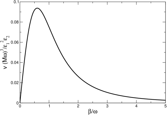
Figure 1: Plot of the current velocity $v$, in units of $\epsilon_{1}^{2}\epsilon_{2}/(M\omega)^{3}$, vs. the damping coefficient $\beta$, in units of the frequency, $\omega$, induced by a biharmonic force like (1) with $\phi_{1}=\phi_{2}=0$. Notice that this force is time reversible, i.e., $f(-t)=f(t)$.

The depence of $v$ on parameters of the system like the damping coefficient (through $\beta=\gamma/M$) shown in (4i) and (4j) reveals an interesting effect. If we take $\phi_{1}=\phi_{2}=0$ in $f(t)$ and do some algebra, the ratchet velocity (for small amplitudes of the force) turns out to be

$$v=\frac{\epsilon_{1}^{2}\epsilon_{2}}{\omega^{3}M^{3}}V(\beta/\omega),\qquad V(x)=\frac{3x(x^{2}+3)}{8(x^{2}+1)^{2}(x^{2}+4)}.$$ (4k)

Function $V(x)$ is depicted in Figure 1. The most remarkable observation is that the current increases up to a maximum with increasing damping before it begins to show the expected decay. Intuition dictates that the current should decrease with damping because friction opposes movement, so the fast increase it reveals for small damping is counterintuitive.

The cause of this effect is the interplay between the breaking of the time-reversal symmetry $\mathcal{R}\,:\,t\mapsto-t$ that generates the ratchet current, and the damping that hinders it [27]. In the limit $\beta\to 0$ the system (4) is invariant under $\mathcal{R}$ and a sign change of $u$, because for $\phi_{1}=\phi_{2}=0$ the force (1) satisfies $f(-t)=f(t)$. Accordingly $v=0$ in this limit. But introducing damping breaks the symmetry of the equation and induces a net movement of the particle. For small damping, the higher the damping coefficient $\beta$ the larger $v$. If we keep on increasing $\beta$ eventually the friction it introduces in the movement of the particle causes the decay of $v$ as $\beta^{-3}$.

This argument makes it clear that in any ratchet system with a tunable damping and undergoing the action of a time-reversible bi-harmonic force, the ratchet effect can be generated upon increasing damping above zero.

4 Ratchet velocity as a functional of the force

The starting point to obtain formula (4i) for a ratchet system is to realize that $v$ is a functional of $f(t)$ and that, under certain regularity assumptions, one such functional can be expanded as a functional Taylor series [28, 29, 30] as

$$v[f]=\sum_{n{\rm\ odd}}\int_{0}^{T}\frac{\rmd t_{1}}{T}\cdots\int_{0}^{T}\frac{\rmd t_{n}}{T}c_{n}(t_{1},\dots,t_{n})f(t_{1})\cdots f(t_{n}),$$ (4l)

where the kernels $c_{n}(t_{1},\dots,t_{n})$ are proportional to the $n$th functional derivatives of the functional $v[f]$. These kernels can be taken $T$-periodic in each variable and totally symmetric under any exchange of variables. Only odd terms appear in this expansion as a cosequence of the symmetry $v[-f]=-v[f]$ that these systems have.

That $v$ is indeed a functional of $f(t)$ in this example is obvious from equations (2)–(4g). The aim of this section is to determine explicitly the expansion (4l) for this exactly solvable example.

Let us start off by rewriting the integral in (4g) as

$$\int_{0}^{t}\rmd zf(z)\rme^{-\beta(t-z)}=I_{1}(t)+I_{2}(t),$$ (4m)

$$I_{1}(t)=\sum_{k=1}^{n(t)}\int_{0}^{T}\rmd zf(z)\rme^{-\beta(t-z-(k-1)T)},$$

$$I_{2}(t)=\int_{0}^{\alpha(t)}\rmd zf(z)\rme^{-\beta(\alpha(t)-z)},$$

where $\alpha(t)=t-n(t)T$ and $n(t)=[t/T]$ ($[X]$ denoting the integer part of $X$). Notice that $\alpha(t+T)=\alpha(t)$. Now, since

$$S(t)\equiv\sum_{k=1}^{n(t)}\rme^{\beta(k-1)T}=\frac{\rme^{\beta nT}-1}{\rme^{\beta T}-1},$$ (4n)

then $I_{1}(t)=\rme^{-\beta t}\,C\,S(t)$, with

$$C=\int_{0}^{T}\rmd zf(z)[\rme^{\beta z}-1].$$ (4o)

Using this form in (4g) we can write

$$P(t)=A\rme^{-\beta t}+\widetilde{P}(t),$$ (4p)

where $A=P(0)+C(\rme^{\beta T}-1)^{-1}$ and $\widetilde{P}(t)$ is the $T$-periodic function

$$\widetilde{P}(t)=-\frac{1}{\rme^{\beta T}-1}\int_{0}^{T}\,\rmd yf(y)\rme^{-\beta\alpha(t)}[\rme^{\beta y}-1]-\int_{0}^{\alpha(t)}\,\rmd yf(y)\rme^{-\beta(\alpha(t)-y)}.$$

It is thus enough to obtain $\widetilde{P}(t)$ in the interval $0\leq t<T$, where it adopts the compact form

$$\widetilde{P}(t)=-\int_{0}^{T}\,\rmd yf(y)\rme^{-\beta(t-y)}\chi(y,t),$$ (4q)

defining

$$\chi(y,t)=\frac{1-\rme^{-\beta y}}{\rme^{\beta T}-1}+\Theta(t-y)$$ (4r)

(as it is customary, $\Theta(x)$ denotes the Heaviside function, which is $1$ if $x>0$ and $0$ otherwise).

Equations (4q)–(4r) have a well defined $\beta\to 0^{+}$ limit, namely

$$\widetilde{P}(t)=-\int_{0}^{T}\,\rmd yf(y)\chi_{1}(y,t),\qquad\chi_{1}(y,t)=\frac{y}{T}+\Theta(t-y).$$ (4s)

On the other hand, for zero-average forces $f(t)$ the kernel $\chi(t,z)$ can be further simplified to

$$\widetilde{P}(t)=-\int_{0}^{T}\,\rmd yf(y)\rme^{-\beta(t-y)}\chi_{2}(y,t),\qquad\chi_{2}(y,t)=\frac{1}{\rme^{\beta T}-1}+\Theta(t-y).$$ (4t)

Whatever the form, it should be periodically extended beyond the interval $[0,T)$.

It is then clear that (2) and (4h) boil down to

$$v=\sum_{k=0}^{\infty}\left(-\frac{1}{2}\right)^{k}\frac{(2k-1)!!}{k!\,M^{2k+1}}\int_{0}^{T}\frac{\rmd\tau}{T}\widetilde{P}(\tau)^{2k+1}.$$ (4u)

A direct comparison of this equation with the functional Taylor series (4l) yields

$$c_{2k}(t_{1},\dots,t_{2k})=0,$$ (4va)

$$c_{2k+1}(t_{1},\dots,t_{2k+1})=\left(-\frac{1}{2}\right)^{k}\frac{(2k-1)!!}{k!\,M^{2k+1}}T^{2k}a_{2k+1}(t_{1},\dots,t_{2k+1}),$$ (4vb)

where

$$a_{m}(t_{1},\dots,t_{m})=\int_{0}^{T}\rmd\tau\,\rme^{-\beta m(\tau-\bar{t})}\prod_{k=1}^{m}\chi(t_{k},\tau),\qquad\bar{t}=\frac{1}{m}\sum_{k=1}^{m}t_{k}.$$ (4vw)

As expected [23], functions $a_{m}(t_{1},\dots,t_{m})$ are, by construction, $T$-periodic in each variable and symmetric under any exchange of their arguments.

The integral in (4vw) can be performed integrating by parts and taking into account that $\frac{d}{d\tau}\chi(y,\tau)=\delta(\tau-y)$ (a Dirac delta). The result is

$$a_{m}(t_{1},\dots,t_{m})=\frac{e^{\beta m\bar{t}}}{\beta m}\left\{\prod_{k=1}^{m}\chi(t_{k},0)-\prod_{k=1}^{m}\chi(t_{k}+T,0)+\sum_{j=1}^{m}e^{-\beta mt_{j}}\prod_{k=1,\ k\neq j}^{m}\chi(t_{k},t_{j})\right\},$$ (4vx)

where we have used the fact that $\chi(t_{k},T)e^{-\beta T}=\chi(t_{k}+T,0)$. As usual, empty products are assumed to be $1$ (the case of the last term for $m=1$).

The limit $\beta\to 0$ of this expression is better obtained by replacing $\chi(y,t)$ by $\chi_{1}(y,t)$ in (4vw) and integrating by parts again. This results in

$$a_{m}(t_{1},\dots,t_{m})=T\prod_{k=1}^{m}\chi_{1}(t_{k},T)-\sum_{j=1}^{m}t_{j}\prod_{k=1,\ k\neq j}^{m}\chi_{1}(t_{k},t_{j}).$$ (4vy)

Finally, in the overdamped case ($M\to 0$, $\beta\to\infty$), instead of (4f) the evolution of $P$ is given by $P(t)=-(1/\beta)f(t)$, so $v$ can be expressed simply as

$$v=-\sum_{k=0}^{\infty}\left(-\frac{1}{2}\right)^{k}\frac{(2k-1)!!}{k!\,\gamma^{2k+1}}\frac{1}{T}\int_{0}^{T}\,\rmd t\,f(t)^{2k+1}.$$ (4vz)

From (4l) and (4vz) it follows that $c_{2k}(t_{1},\dots,t_{2k})=0$ and

$$c_{2k+1}(t_{1},\dots,t_{2k+1})=-\left(-\frac{T^{2}}{2}\right)^{k}\frac{(2k-1)!!}{k!\,\gamma^{2k+1}}\,\delta(t_{1}-t_{2})\cdots\delta(t_{2k}-t_{2k+1}).$$ (4vaa)

4.1 Forcing with a time-periodic piecewise constant force

The expansion (4l) with kernels (4vb) and (4vw) turns out to be useful to analyze different types of forcing. For instance, another standard choice in the literature (see [1] and references therein), alongside with the bi-harmonic force (1), has been the time-periodic piecewise constant force defined in (3). This force is shift-symmetric only for $T_{l}=T/2$, so any other value $T_{l}<T/2$ breaks this symmetry and induces a ratchet current.

In order to ascertain the effect of this force in system (4b) for small amplitudes $\epsilon_{1}\ll 1$, we will compute the first nonzero term in the expansion (4l). To that purpose we need to evaluate (c.f. equation (4vw))

$$K_{m}\equiv\langle a_{m}(t_{1},\dots,t_{m})f(t_{1})\cdots f(t_{m})\rangle=\int_{0}^{T}\left[e^{-\beta\tau}I(\tau)\right]^{m}d\tau,$$ (4vaba)

$$I(\tau)\equiv\frac{1}{T}\int_{0}^{T}e^{\beta t}\chi_{2}(t,\tau)f(t)\,dt,$$ (4vabb)

where the choice $\chi_{2}(t,\tau)$ instead of $\chi(t,\tau)$ is made because $f(t)$ in (3) has zero average. According to (4t) $\chi_{2}(t,\tau)=(1-e^{-\beta T})^{-1}\bar{\chi}_{2}(t,\tau)$, where

$$\bar{\chi}_{2}(t,\tau)=\cases{1&\text{if $t<\tau$,}\\ e^{-\beta T}&\text{if $t>\tau$.}}$$ (4vabac)

Substitution into (4vabb) yields

$$I(\tau)=\frac{\epsilon_{1}}{\beta T}\left[\frac{4}{1-e^{-\beta T}}\sinh^{2}\left(\frac{\beta T_{l}}{2}\right)+Q(\tau)\right],$$ (4vabada)

$$Q(\tau)=\cases{e^{\beta\tau}-e^{\beta T_{l}}&\text{if $0<\tau<T_{l}$,}\\ 0&\text{if $T_{l}<\tau<T-T_{l}$,}\\ e^{\beta(T-T_{l})}-e^{\beta\tau}&\text{if $T-T_{l}<\tau<T$.}\\ }$$ (4vabadb)

It is straightforward to check that $K_{1}$ in (4vaba) vanishes, so the first term that may not be zero is $K_{3}$. Lengthy calculations lead to

$$K_{3}=-\frac{32\epsilon_{1}^{3}}{\beta^{4}T^{3}}\,\frac{e^{\beta T}}{(e^{\beta T}-1)^{2}}\sinh^{2}\left(\frac{\beta(T-2T_{l})}{2}\right)\sinh^{4}\left(\frac{\beta T_{l}}{2}\right),$$ (4vabadae)

that is to say

$$v=\frac{4\epsilon_{1}^{3}}{(\beta M)^{3}\beta T}\sinh^{2}\left(\frac{\beta(T-2T_{l})}{2}\right)\frac{\sinh^{4}\left(\beta T_{l}/2\right)}{\sinh^{2}\left(\beta T/2\right)}+o(\epsilon_{1}^{3}).$$ (4vabadaf)

It is interesting to noticing that $K_{3}=0$ if $T_{l}=T/2$ because in that case the time-periodic piecewise constant force (3) is shift-symmetric. On the other hand, we can determine the value of $T_{l}$ for which the ratchet effect is maximum by differetiating (4vabadaf). This leads to

$$\sinh\left(\frac{\beta(T-3T_{l})}{2}\right)\sinh\left(\frac{\beta(T-2T_{l})}{2}\right)\sinh^{3}\left(\frac{\beta T_{l}}{2}\right)=0.$$ (4vabadag)

The only three solutions to this equation are $T_{l}=0$, $T_{l}=T/2$ and $T_{l}=T/3$. The first two do not produce any ratchet current (with $T_{l}=0$ $f=0$ whereas for $T_{l}=T/2$ the force is shift-symmetric), therefore the last one provides its maximum value.

As a final remark, expression (4vabadaf) has well defined overdamped ($M\to 0$, $\beta\to\infty$, with finite $\gamma=\beta M$) and undamped ($\beta\to 0$) limits. In fact, the undamped limit of (4vabadaf) yields

$$v=\frac{\epsilon_{1}^{3}}{4(MT)^{3}}T_{l}^{4}(T-2T_{l})^{2}+o(\epsilon_{1}^{3}),$$ (4vabadah)

whereas the overdamped produces $v=o(\epsilon_{1}^{3})$. Indeed, since $f(t)^{2k+1}=\epsilon_{1}^{2k}f(t)$, in the overdamped case Eq. (4vz) immediately implies $v=0$. This is in marked contrast with the overdamped deterministic dynamic of a particle in a sinusoidal potential driven by a bi-harmonic force [31]. In this case, the zero ratchet velocity can be explained as a symmetry effect. Indeed, notice that $f(t)=-f(-t)$ when $f(t)$ is given by (3) (something that only happens for the bi-harmonic force (1) for specific choices of the phases), and that the overdamped limit of Eq. (4b) remains invariant under a simultaneously action of time-reversal and a sign change of $x$ and $u$ (see [23] for further details).

5 Discussion

We have studied the dynamics of a damped relativistic particle under two zero average $T$-periodic forces which breaks the shift-symmetry $f(t+T/2)=-f(t)$. This nonlinear system can be explicitly solved through a transformation that renders it linear. Therefore, the ratchet average velocity, $v$, is exactly obtained for any arbitrary force $f(t)$. This result allows us to show, first of all, that the ratchet velocity cannot be obtained in general by using the method of moments (according to which $v$ is obtained as a series of the odd moments of $f(t)$). And secondly, that $v$ is a functional of $f(t)$, i.e. $v[f]$. Indeed, for any $T$-periodic force we have explicitly found the coefficients of the functional Taylor expansion (4l). In particular, this expansion shows that the method of moments is only justified in the strict overdamped limit (see Eqs. (4vz) and (4vaa)). Due to the symmetry $v[f]=-v[-f]$ only odd terms contribute to the Taylor expansion. Besides, since the ratchet velocity is translationally invariant, the kernel $c_{1}(t_{1})$ must be a constant. So the first order term vanishes because the force has zero average. Therefore, the first term in the expansion (4l) that is not necessarily zero is the third one, irrespective of the kind of nonlinearity of the system.

We have chosen to illustrate this functional representation the bi-harmonic force (1) (with $p=2$ and $q=1$) as well as a time-periodic piecewise constant force (3). We have obtained the leading term of the average velocity for both these forces. They are given by equations (4i)–(4j) and (4vabadaf), respectively. It is worth emphasizing that the method of moments always predicts a zero ratchet velocity when the system is driven by a time-periodic piecewise constant. This is to be compared with the result (4vabadaf) obtained here. We have discussed the two limiting dynamics: undamped and overdamped. In these two limits the system remains invariant if the driving force has the symmetries $f(t)=f(-t)$ and $f(t)=-f(-t)$, respectively. If the relativistic particle is driven by a bi-harmonic force $v\sim\epsilon_{1}^{2}\epsilon_{2}\cos(2\phi_{1}-\phi_{2})$ in the overdamped limit, whereas $v\sim\epsilon_{1}^{2}\epsilon_{2}\sin(2\phi_{1}-\phi_{2})$ in the undamped limit. In the latter case this means no ratchet current if we set $\phi_{1}=\phi_{2}=0$. The unexpected consequence of this is that introducing damping generates a ratchet current, whose intensity grows up to a maximum before it drops to zero upon a further increase of the damping. This effect is a result of a trade off between symmetry effects and friction and our prediction is that should be observed in any system with damping and forced with a time-reversible external force.

On its side, if an overdamped relativistic particle is driven by a time-periodic piecewise constant force like (3), the ratchet velocity is always zero as a consequence of the symmetry $f(t)=-f(-t)$ exhibited by this force.

Summarizing, we hope to have illustrated the predictive power of the Taylor functional expansion method introduced in [23]. This working example also shows that this is the only reliable method to analyze the ratchet current as a function of the parameters of the external force. The most widely used alternative so far, the method of moments, is shown to work only in the overdamped limit of the dynamics of a relativistic particle driven by a periodic force. When damping is finite and the forcing of the system is bi-harmonic, the rathet current predicted by the method of moments still retains some relevant features of the exact one (4i). However, it dramatically fails if the system is driven by a piecewise constant force, because it always predicts a zero ratchet current, in marked constrast with the result (4vabadaf) predicted by the functional Taylor expansion.

References

References

• [1] P. Reimann. Phys. Rep., 361:57, 2002.
• [2] M. Salerno and N. R. Quintero. Soliton ratchets. Phys. Rev. E, 65:025602(R), 2002.
• [3] M. O. Magnasco. Phys. Rev. Lett., 71:1477, 1993.
• [4] F. Falo, P. J. Martínez, J. J. Mazo, T. P. Orlando, K. Segall, and E. Trías. Appl. Phys. A, 75:263, 2002.
• [5] P. Reimann and P. Hänggi. Appl. Phys. A, 75:169, 2002.
• [6] R. D. Astumian and P. Hänggi. Phys. Today, 55:32, 2002.
• [7] H. Linke, editor. Ratchets and Brownian motors: basics, experiments and applications, volume 75 of Appl. Phys. A Special Issues. 2002.
• [8] J. E. Villegas, S. Savel’ev, F. Nori, E. M. González, J. V. Anguita, R. García, and J. L. Vicent. Science, 302:1188, 2003.
• [9] M. Beck, E. Goldobin, M. Neuhaus, M. Siegel, R. Kleiner, and D. Koelle. Phys. Rev. Lett., 95:090603, 2005.
• [10] P. Hänggi and F. Marchesoni. Rev. Mod. Phys., 81:387, 2009.
• [11] W. Schneider and K. Seeger. Appl. Phys. Lett., 8:133, 1966.
• [12] A. Ajdari, D. Mukamel, L. Peliti, and J. Prost. J. Phys. I France, 4:1551, 1994.
• [13] A. Engel, H. W. Müller, P. Reimann, and A. Jung. Phys. Rev. Lett., 91:060602, 2003.
• [14] L. Morales-Molina, N. R. Quintero, F. G. Mertens, and A. Sánchez. Phys. Rev. Lett., 91:234102, 2003.
• [15] M. Schiavoni, L. Sánchez-Palencia, F. Renzoni, and G. Grynberg. Phys. Rev. Lett., 90:094101, 2003.
• [16] A. V. Ustinov, C. Coqui, A. Kemp, Y. Zolotaryuk, and M. Salerno. Phys. Rev. Lett., 93:087001, 2004.
• [17] D. Cole, S. Bending, S. Savel’ev, A. Grigorenko, T. Tamegai, and F. Nori. Nat. Mater., 5:305, 2006.
• [18] S. Ooi, S. Savel’ev, M. B. Gaifullin, T. Mochiku, K. Hirata, and F. Nori. Phys. Rev. Lett., 99:207003, 2007.
• [19] P. Curie. J. Phys. (Paris) Sér. 3, III:393, 1894.
• [20] J. Ismael. Curie’s principle. Synthese, 110:167–190, 1997.
• [21] S. Flach, O. Yevtushenko, and Y. Zolotaryuk. Phys. Rev. Lett., 84:2358, 2000.
• [22] M. Salerno and Y. Zolotaryuk. Phys. Rev. E, 65:056603, 2002.
• [23] N. R. Quintero, J. A. Cuesta, and R. Alvarez-Nodarse. Symmetries shape the current in ratchets induced by a bi-harmonic force. Phys. Rev. E, 81:030102R, 2010.
• [24] C. E. Skov and E. Pearlstein. Rev. Sci. Inst., 35:962, 1964.
• [25] S. Denisov, S. Flach, A. A. Ovchinnikov, O. Yevtushenko, and Y. Zolotaryuk. Phys. Rev. E, 66:041104, 2002.
• [26] O. H. Olsen and M. R. Samuelsen. Phys. Rev. B, 28:210, 1983.
• [27] L. Morales-Molina, N. R. Quintero, A. Sánchez, and F. G. Mertens. Chaos, 16:013117, 2006.
• [28] R. F. Curtain and A. J. Pritchard. Functional Analysis in Modern Applied Mathematics. Academic Press, London, 1977.
• [29] J. J. Binney, N. J. Dowrick, A. J. Fisher, and M. E. J. Newman. The Theory of Critical Phenomena: An Introduction to the Renormalization Group. Oxford University Press, Oxford, 1992.
• [30] J. P. Hansen and I. R. McDonald. Theory of Simple Liquids. Academic Press, London, 3rd edition, 2006.
• [31] V. Lebedev D. Cubero and F. Renzoni. Current reversals in a rocking ratchet: Dynamical versus symmetry-breaking mechanisms. Phys. Rev. E, 82:041116, 2010.