Unitary Application of the Quantum Error Correction Codes

Abstract

From the set of operators for errors and its correction code, we introduce the so-called complete unitary transformation. It can be used for encoding while the inverse of it can be applied for correcting the errors of the encoded qubit. We show that this unitary protocol can be applied for any code which satisfies the quantum error correction condition.

In quantum computation and communication, quantum error correction (QEC) will be necessary for preserving coherent states against noise and other unwanted interaction. Based on the classic schemes using redundancy, Shor [1] has championed a strategy where a bit of quantum information is stored in an entanglement of nine qubits. This scheme permits one to correct for any error incurred by any of the nine qubits. For the same purpose, Steane [2] has proposed a protocol which uses seven qubits. Five qubit has the minimum size for a quantum code which encodes a single qubit so that any error on a single qubit in the encoded state can be detected and recovered. The five qubit code was discovered by Bennett, DiVincenzo, Smolin and Wootters [3], and independently by Laflamme, Miquel, Paz and Zurek [4]. The quantum error-correction conditions were proved independently by Bennett and co-authors [3], and by Knill and Laflamme [5].

The above protocols with different quantum error correction codes (QECCs) can be viewed as active error correction. There are passive error avoiding techniques such as the decoherence-free subspaces [6-8] and noiseless subsystem [9-11]. Recently, it was found that all the active and passive QEC methods can be unified together[12-14].

The standard way of applying the known quantum error-correcting codes (QECCs) for error-correcting contains: encoding procedure $\mathcal{C}$, the noise channel $\mathcal{\varepsilon}$, and the recovery operation $\mathcal{R}$. Considering the joint system $A\otimes B$, where $\{|e_{i}\rangle\}_{i=0,1,...,M}$ is the basis of the ancilla system A while $\{|0\rangle,|1\rangle\}$ is the basis of the principle system B, the encoding procedure can be realized with an unitary transformation U,

$$U|e_{0}\rangle\otimes|0\rangle\rightarrow|0_{L}\rangle,U|e_{0}\rangle\otimes|1\rangle\rightarrow|1_{L}\rangle.$$ (1)

Let $\rho^{\texttt{in}}$ denote the input state,

$$\rho^{\texttt{in}}=|e_{0}\rangle\langle e_{0}|\otimes|\psi\rangle\langle\psi|,|\psi\rangle=\alpha|0\rangle+\beta|1\rangle,$$ (2)

after the operations of $\varepsilon$ and $\mathcal{R}$, the output state $\rho^{\texttt{out}}$ is known,

$$\rho^{\texttt{out}}=(\mathcal{R}\circ\varepsilon)(U\rho^{\texttt{in}}U^{\dagger})=|\Phi\rangle\langle\Phi|,$$ (3)

where $|\Phi\rangle=\alpha|0_{L}\rangle+\beta|1_{L}\rangle.$ This standard QEC protocol is usually non-unitary: the recovery operation $\mathcal{R}$ should transfer the mixture $\varepsilon(U\rho^{\texttt{in}}U^{\dagger})$ into the pure state $|\Phi\rangle\langle\Phi|$. A different but unitary scheme has been presented by Laflamme and co-authors. They designed a five-qubit code and showed that the errors of the encoded qubit can be corrected with a series of unitary transformations [4].

In the present work, we shall develop an unitary protocol to apply the known perfect codes for quantum error correction. We introduce the concept of complete unitary transformation $\tilde{U}$ which can be decided by the code and the set of operators for errors. In the unitary QEC protocol, $\tilde{U}$ is used for encoding while its inverse $\tilde{U}^{\dagger}$ is sufficient for correcting the errors of the encoded qubit. Compared with the standard QEC protocol, it leaves the errors of the ancilla system to be un-corrected. The content of our work can be divided into three parts. At first, we shall give a brief review for the work of Laflamme and co-authors in [4], and generalize their work into the unitary protocol where $\tilde{U}$ works. Then, we find a general method to introduce $\tilde{U}$ and show that the unitary QEC protocol, which is originated from the scheme in [4], can be applied for any code satisfying the quantum error correction condition. Finally, we show that our protocol is consistent with the unified model of QEC developed by Kribs, Laflamme and Paulin in [12].

To protect a qubit of information against the general one qubit errors, Laflamme and co-authors presented the following five-qubits code,

$$|0_{L}\rangle= -|00000\rangle+|01111\rangle-|10011\rangle+|11100\rangle$$

$$+|00110\rangle+|01001\rangle+|10101\rangle+|11010\rangle,$$

$$|1_{L}\rangle= -|11111\rangle+|10000\rangle+|01100\rangle-|00011\rangle$$ (4)

$$+|11001\rangle+|10110\rangle-|01010\rangle-|00101\rangle.$$

They designed the quantum circuit for encoding and used the same circuit running backwards for error-correcting. Their scheme is organized in Fig. 1a. Let the operators of errors are denoted by $\varepsilon:\{\sqrt{p_{m}}E_{m}\}_{m=0.1,...,M}$, with $\langle\Phi|E^{\dagger}_{m}E_{m}|\Phi\rangle=1$, the U in Fig. 1a has the property that

$$(\texttt{a})~{}~{}~{}U|e_{0}\rangle\otimes|\psi\rangle\rightarrow\alpha|0_{L}\rangle+\beta|1_{L}\rangle,$$

$$(\texttt{b})~{}~{}~{}U^{\dagger}E_{m}U|e_{0}\rangle\otimes|\psi\rangle=|e_{m}\rangle\otimes|\psi_{m}\rangle,$$

where the state $|\psi_{m}\rangle$ is known,

$$|\psi_{m}\rangle\in\{\pm(\alpha|0\rangle+\beta|1\rangle),\beta|0\rangle\pm\alpha|1\rangle,\pm(\alpha|0\rangle-\beta|1\rangle)\}.$$

Usually, we fix $E_{0}=\texttt{{I}}$, and there should be $|\psi_{0}\rangle=|\psi\rangle$. The scheme in Fig. 1a works in the way like

$$\rho^{\texttt{out}}=U^{\dagger}[\varepsilon(U\rho^{\texttt{in}}U^{\dagger})]U=\sum_{m=0}^{M}p_{m}|e_{m}\rangle\langle e_{m}|\otimes|\psi_{m}\rangle\langle\psi_{m}|.$$

From it, the original state of the principle system can then be restored by the successive unitary transformation $U_{\delta}^{\dagger}$,

$$U_{\delta}^{\dagger}|e_{m}\rangle\otimes|\psi_{m}\rangle\rightarrow|e_{m}\rangle\otimes|\psi\rangle.$$

This $U_{\delta}^{\dagger}$ has been suggested in the original work, the circuit for it has not been given there. As we shall show later, it can be easily designed.

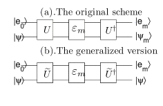
Figure 1: (a) The scheme of the original work in [4]. $U^{\dagger}$ is called the error finder there, it is realized by the same circuit of U running backwards. (b) For the five qubit code in (4), we define $\tilde{U}=U\cdot U_{\delta}$ with $U_{\delta}$ defined as $U^{\dagger}_{\delta}|e_{m}\rangle\otimes|\psi_{m}\rangle\rightarrow|e_{m}\rangle\otimes|\psi\rangle.$ Noting $U_{\delta}$ has been suggested in [4] but its circuit was not given there. For other perfect codes, the $\tilde{U}$ can be introduced by the general method in (11)

Jointing the two unitary $U$ and $U_{\delta}$ together, we could define the complete unitary transformation $\tilde{U}$,

$$\tilde{U}=U\cdot U_{\delta},\tilde{U}^{\dagger}=U_{\delta}^{\dagger}\cdot U^{\dagger}.$$ (5)

Noting $U_{\delta}^{\dagger}|e_{m}\rangle\otimes|\psi_{m}\rangle\rightarrow|e_{m}\rangle\otimes|\psi\rangle$, with $U_{\delta}U_{{\delta}}^{\dagger}=\texttt{{I}}$, there should be $U_{\delta}|e_{m}\rangle\otimes|\psi\rangle\rightarrow|e_{m}\rangle\otimes|\psi_{m}\rangle$. Jointing it with the known property of U, one may easily verify that $\tilde{U}$ has the following two properties:

$$\tilde{U}|e_{0}\rangle\otimes|\psi\rangle\rightarrow\alpha|0_{L}\rangle+\beta|1_{L}\rangle,$$ (6)

$$\tilde{U}^{\dagger}E_{m}\tilde{U}|e_{0}\rangle\otimes|\psi\rangle=|e_{m}\rangle\otimes|\psi\rangle.$$ (7)

The result in (6) shows that $\tilde{U}$ can be used for encoding and the one in (7) permits us to correct the errors of the encoded qubit with $\tilde{U}^{\dagger}$. All these results are depicted in fig. 1b where the total process can be described with

$$\rho^{\texttt{out}}=\tilde{U}^{\dagger}[\varepsilon(\tilde{U}\rho^{\texttt{in}}\tilde{U}^{\dagger})]\tilde{U}=\sum_{m=0}^{M}p_{m}|e_{m}\rangle\langle e_{m}|\otimes|\psi\rangle\langle\psi|.$$ (8)

Compared with the standard QEC protocol, the errors of the ancilla system are not corrected here.

As a key step to show that the unitary protocol in Fig. 1b can be applied for other perfect codes, we note that the way of introducing $\tilde{U}$ is non-unique. Besides the way in (5), we find it can be also decided by the code in (4) and the operators of errors. Let’s introduce the denotation,

$$|0,+\rangle\equiv|0_{L}\rangle,|0,-\rangle\equiv|1_{L}\rangle,$$ (9)

and define

$$E_{m}|0,+\rangle=|m,+\rangle,E_{m}|0,-\rangle=|m,-\rangle.$$ (10)

An interpretation for our denotation above is shown in Fig. 2. With the code in (4) and the known sixteen operators of errors, one may prove that the set of states, $\{|m,\pm\rangle\}_{m=0,1,...,15}$, form an orthogonal basis. Furthermore, one may also verify that the complete $\tilde{U}$ in (5) is just the unitary transformation between the two sets of basis, $\{|e_{m}\rangle\otimes|0\rangle,|e_{m}\rangle\otimes|1\rangle\}_{m}$ and $\{|m,\pm\rangle\}_{m}$, here,

$$\tilde{U}|e_{m}\rangle\otimes\left(\begin{array}[]{c}|0\rangle\\ |1\rangle\\ \end{array}\right)\rightarrow\left(\begin{array}[]{c}|m,+\rangle\\ |m.-\rangle\\ \end{array}\right).$$ (11)

Under the unitary condition that $\tilde{U}\tilde{U}^{\dagger}=\texttt{{I}}$, there should be

$$\tilde{U}^{\dagger}\left(\begin{array}[]{c}|m,+\rangle\\ |m.-\rangle\\ \end{array}\right)\rightarrow|e_{m}\rangle\otimes\left(\begin{array}[]{c}|0\rangle\\ |1\rangle\\ \end{array}\right).$$ (12)

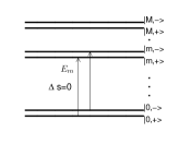
Figure 2: The atomic model for QEC. We use $|m.s\rangle$ to denote the level of the atom where m is the integer for energy while s is the number of spin, $s=\pm 1$. Taking $|0,\pm\rangle$ for the ground state, it will be transited to the $m-th$ level under the action of $E_{m}$. In this picture, the qubit of information is stored in the internal degree of spin and this information is protected since that all the transitions should obey the rule $\Delta s=0$.

The way of introducing $\tilde{U}$ in (11) is obviously general: For a given code and its corresponding set of errors $\{\sqrt{p_{m}}E_{m}\}_{m=0,1,...,M}$, we can always introduce the set of states, $\{|m,\pm\rangle\}_{m=0,1,...,M}$, by following the steps in (9) and (10). This set of states should formulate an orthogonal basis, as we shall show later, if the code satisfies the quantum error correction condition. Noting the basis, $\{|e_{m}\rangle\otimes|0\rangle,|e_{m}\rangle\otimes|1\rangle\}$, has also been given. In principle, one may get $\tilde{U}$ from (11) and design the quantum circuit for it. In following, we shall organize the above argument with a strict proof: For any code which satisfies the perfect error-correcting condition

$$\hat{P}_{C}E^{\dagger}_{m}E_{n}\hat{P}_{c}=\delta_{mn}\hat{P}_{C}$$ (13)

where the projection operator $\hat{P}_{C}$ is defined as $\hat{P}_{C}=|0,+\rangle\langle 0,+|+|0,-\rangle\langle 0,-|$, we have $\hat{P}_{C}E^{\dagger}_{m}E_{n}\hat{P}_{C}=(|0,+\rangle\langle m,+|+|0,-\rangle\langle m,-|)(|n,+\rangle\langle 0,+|+|n,-\rangle\langle 0,-|)$. Introducing the following four Hermitian operators, $\hat{O}_{1}=|0,+\rangle\langle 0,+|$, $\hat{O}_{2}=|0,-\rangle\langle 0,-|$, $\hat{O}_{3}=|0,+\rangle\langle 0,-|+|0,-\rangle\langle 0,+|$, and $\hat{O}_{4}=i|0,+\rangle\langle 0,-|-i|0,-\rangle\langle 0,+|$, we could perform the four calculations $\texttt{Tr}[\hat{O}_{i}(\cdot)]$ on the both sides of equation (13) and get the results,

$$\langle m,+|n,+\rangle=\langle m,-|n,-\rangle=\delta_{mn},$$

$$\langle m,+|n,-\rangle=\langle m,-|n,+\rangle=0,$$ (14)

which are sufficient to show that the set of states $\{|m,\pm\rangle\}_{m=0,1,...,M}$ formulate an orthogonal basis. With the $\tilde{U}$ from (11), we are able to show that the general scheme in Fig. 1b works for any perfect code. First, with $|\psi\rangle=\alpha|0\rangle+\beta|1\rangle$ and equation (11), we recover the result in (6), $\tilde{U}|e_{0}\rangle\otimes|\psi\rangle\rightarrow\alpha|0,+\rangle+\beta|0,-\rangle$. Suppose that the error $E_{m}$ happens, from the denotation in (10), there is $E_{m}\tilde{U}|e_{0}\rangle=\alpha|m,+\rangle+\beta|m,-\rangle$. After the action of $\tilde{U}^{\dagger}$ in (12), we have $\tilde{U}^{\dagger}E_{m}\tilde{U}|e_{0}\rangle=|e_{m}\rangle\otimes|\psi\rangle$, the same result given in (7). Noting that the conditions in (6) and (7) are sufficient for error-correcting of the principle system B, we conclude that any perfect QECCs can be applied for error correction in the unitary way shown in Fig. 1b.

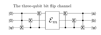
Figure 3: The circuit for the three binary flip cannel in [15]. Noting the circuit for encoding and the circuit of error-correcting have a mirror symmetry.

It should be noted that $\tilde{U}$ is not unique. This can be seen from the three qubit bit flip channel in [15]. Letting $|e_{0}\rangle=|00\rangle$, $|e_{1}\rangle=|01\rangle$, $|e_{2}\rangle=|10\rangle$, $|e_{3}\rangle=|11\rangle$, and fixing $E_{0}=I^{\otimes 3}$, we still have the freedom in defining the sequence of the operators. For example, the following two choices, (I) $E_{1}=\hat{X}\otimes\texttt{{I}}\otimes\texttt{{I}}$, $E_{2}=\textbf{{I}}\otimes\ \hat{X}\otimes\texttt{{I}}$, $E_{3}=\texttt{{I}}\otimes\textbf{{I}}\otimes\ \hat{X}$ and (II) $E_{1}=\textbf{{I}}\otimes\ \hat{X}\otimes\texttt{{I}}$, $E_{2}=\hat{X}\otimes\texttt{{I}}\otimes\texttt{{I}}$, $E_{3}=\texttt{{I}}\otimes\textbf{{I}}\otimes\ \hat{X}$, will lead two different $\tilde{U}$ which can both be applied for Fig. 1b. However, the circuits for them are different. So, the sequence of the operators should be specified when the quantum circuit for $\tilde{U}$ is to be designed. The circuit in Fig. 3 is for the three-qubit bit flip channel with $|0_{L}\rangle=|000\rangle$, $|1_{L}\rangle=|111\rangle$, and the sequence of the operators in (I) above. The circuit in Fig. 4 is constructed for the five-qubit code,

$$|0_{L}\rangle = -|00000\rangle+|00101\rangle+|01010\rangle+|01111\rangle$$

$$+ |10011\rangle-|10110\rangle+|11001\rangle+|11100\rangle$$

$$|1_{L}\rangle = -|00011\rangle-|00110\rangle+|01001\rangle-|01100\rangle$$ (15)

$$+ |10000\rangle+|10101\rangle+|11010\rangle-|11111\rangle,$$

which is get from the code in (4) by moving the third qubit to the final location. The sequence of the operators is:

$$\hat{I},\hat{X}_{4},\hat{Z}_{3},\hat{X}_{5},\hat{Z}_{2},\hat{Y}_{3},\hat{X}_{1},\hat{X}_{3},\hat{Z}_{1},\hat{Y}_{5},\hat{Z}_{5},\hat{X}_{2},\hat{Z}_{4},\hat{Y}_{4},\hat{Y}_{1},\hat{Y}_{2},$$

while the basis vectors $|e_{m}\rangle$ are fixed as $|e_{0}\rangle=|0000\rangle$, $|e_{1}\rangle=|0001\rangle$, $|e_{2}\rangle=|0010\rangle$,…, $|e_{15}\rangle=|1111\rangle$.

Figure 4: In the original circuit for the five qubit code in (4), the information is encoded in the third qubit. In the present work, we use the code in (15) and encode the qubit of information in the final location. The part of circuit, which is within the dash lines, plays the role of $U$ in Fig. 1a. It is designed in the similar way of [4]. H is used for the Hadamard gate. The filled circle denotes the control is $|1\rangle$ while the empty one is for $|0\rangle$. $\pi$ is the global phase shift $\exp\{i\pi\}$ in short. $\tilde{U}^{\dagger}$ is not given here, it can be easily constructed by letting the above circuit run backwards.

Considering the fact that both the $\tilde{U}$ and $\varepsilon:\{\sqrt{p_{m}}E_{m}\}$ are known, we could introduce the so-called transformed operators,

$$\tilde{E}_{m}=\tilde{U}^{\dagger}E_{m}\tilde{U},$$ (16)

and define the transformed channel as $\tilde{\varepsilon}:\{\sqrt{p_{m}}\tilde{E}_{m}\}$ with $\langle\Phi|\tilde{E}_{m}^{\dagger}\tilde{E}_{m}|\Phi\rangle=1.$ Certainly, there should be

$$\tilde{E}_{m}|e_{0}\rangle\otimes|\psi\rangle=|e_{m}\rangle\otimes|\psi\rangle.$$ (17)

Now, the process in Fig. 1b can be expressed with the compact form

$$\rho^{\texttt{out}}=\tilde{\varepsilon}(\rho^{\texttt{in}})=\sum_{m=0}^{M}p_{m}\tilde{E}_{m}\rho^{\texttt{in}}\tilde{E}_{m}^{\dagger}.$$ (18)

Certainly, $\rho^{\texttt{out}}=\sum_{m=0}^{M}p_{m}|e_{m}\rangle\langle e_{m}|\otimes|\psi\rangle\langle\psi|$. As it is shown in [12], the QEC with perfect codes can be unified with other QEC protocols like the decoherence-free subspaces and the noiseless subsystems. The unified scheme for quantum error-correction consists of a triple $(\mathcal{R},\varepsilon,\mathscr{U})$, $\mathscr{U}$ is correctable for $\varepsilon$ if

$$(\texttt{Tr}_{\texttt{A}}\circ\mathcal{P}_{\mathscr{U}}\circ\mathcal{R}\circ\varepsilon)(\rho)=\texttt{Tr}_{\texttt{A}}(\rho).$$ (19)

It can be shown that $\tilde{\varepsilon}$ is consistent with this unified scheme. At first, we introduce the decomposition of the joint system $A\otimes B$, $\mathcal{H}=(\mathcal{H}^{\texttt{A}}\otimes\mathcal{H}^{\texttt{B}})\oplus\mathcal{K}$, where the basis for each subspace is known: $\mathcal{H}^{\texttt{A}}$ is one-dimensional with $|e_{0}\rangle$, $\mathcal{H}^{\texttt{B}}$ is with its basis as $\{|0\rangle,|1\rangle\}$, and $\mathcal{K}$ has its basis to be $\{|e_{m}\rangle\otimes 0\rangle,|e_{m}\rangle\otimes|1\rangle\}$ for $m\geq 1$. Then, we could define a set of operators

$$\mathscr{U}=\{\rho\in\mathcal{B}(\mathcal{H}),\rho=|e_{0}\rangle\langle e_{0}|\otimes\rho^{\texttt{B}}\}$$ (20)

where $\rho^{\texttt{B}}$ is an arbitrary state of the principle system B. With $\hat{P}_{\mathscr{U}}=|e_{0}\rangle\langle e_{0}|\otimes(|0\rangle\langle 0|+|1\rangle\langle 1|)$, we have $\hat{P}_{\mathscr{U}}\mathcal{H}=\mathcal{H}^{\texttt{A}}\otimes\mathcal{H}^{\texttt{B}}$. Let $\mathcal{P}_{\mathscr{U}}=\hat{P}_{\mathscr{U}}(\cdot)\hat{P}_{\mathscr{U}}$, we find that our protocol in (18) could be expressed as

$$(\texttt{Tr}_{\texttt{A}}\circ\mathcal{P}_{\mathscr{U}}\circ\tilde{\varepsilon})(\rho)=\texttt{Tr}_{\texttt{A}}(\rho),\forall{\rho}\in\mathscr{U}.$$ (21)

In other words, it is captured in the unified scheme with the recovery operation $\mathcal{R}=\texttt{{I}}$.

For simplicity, we have expressed the operators of the errors with the form $\{\sqrt{p_{m}}E_{m}\}$. This denotation is strict if the code saturates the quantum Hamming bound. For the more general case, one may introduce an extra index besides the subscript m for the operators, say , $E^{\alpha_{m}}_{m}$, and let $\{E_{m}^{\alpha_{m}}\}$ denote the subset of the operators whose action on $|0,\pm\rangle$ will lead to the same state, $E_{m}^{\alpha_{m}}|0,\pm\rangle=|m,\pm\rangle$. This substitution, $E_{m}\rightarrow E_{m}^{\alpha_{m}}$, will not change the results above.

With a simple program, we have got the complete $\tilde{U}$ corresponding to the Shor’s nine qubit code, Steane’s seven qubit code, and the five qubit code of Bennett and co-authors. For each $\tilde{U}$, we have calculated all the deformed Kraus operators, $\tilde{U}^{\dagger}E_{m}\tilde{U}$, and verified that the result in (16) always holds. The quantum circuit for these complete unitary transformation are still under researching. Suppose the designed circuit has been realized in experiment, one could perform the standard quantum process tomography (SQPT) over the channel of the encoded qubit [15]. With the experimental data about the four final states of system B, which correspond to the set of input states, $|e_{0}\rangle\otimes|\phi_{j}\rangle$ with $\forall|\phi_{j}\rangle\in\{|0\rangle,|1\rangle,\frac{\sqrt{2}}{2}(|0\rangle+|1\rangle),\frac{\sqrt{2}}{2}(|0\rangle+i|1\rangle)\}$, one may easily judge whether the channel of B is perfect or not.

Compared with the standard QEC protocol, the scheme in Fig. 1b does not require the errors in the ancilla system to be corrected. In some aspects, our scheme is very similar with the passive QEC protocols where the recovery operation $\mathcal{R}$ takes a trivial form. As a known result, any code satisfying the quantum error-correction condition in (13) can be used in the standard QEC protocol. For the same code, we offer another choice of applying it for quantum error correction.

We would like to acknowledge the help discussion with Prof. Cen L.-X.

References

• (1) P. Shor, Phys. Rev. A 52, 2493(1995).
• (2) A. M. Steane, Phys. Rev. Lett. 77, 793(1996).
• (3) C. H. Bennett, D. P. DiVincenzo, J. A. Smolin, and W. K. Wootters, Phys. Rev. A 54, 3824(1996).
• (4) R. Laflamme, C. Miquel, J. P. Paz, and W. H. Zurek, Phys. Rev. Lett. 77, 198(1996).
• (5) E. Knill and R. Laflamme, Phys. Rev. A 55, 900(1997).
• (6) L.-M. Duan and G.-C. Guo, Phys. Rev. Lett. 79, 1953(1997).
• (7) D. Lidar, I. Chuang, and K. Whaley, Phys. Rev. Lett. 81, 2594(1998).
• (8) P. Zanardi and M. Rasetti, Phys. Rev. Lett. 79, 3306(1997).
• (9) E. Knill, R. Laflamme, and L.Viola, Phys. Rev. Lett. 84, 2525(2000).
• (10) P. Zanardi, Phys. Rev. A 63,12301(2000).
• (11) J. Kempe, D. Bacon, D. A. Lidar, and K. B. Whaley, Phys. Rev. A 63, 42307(2001).
• (12) D. Kribs, R. Laflamme, and D. Poulin, Phys. Rev. Lett. 94, 180501(2005).
• (13) D. Poulin, Phys. Rev. Lett. 95, 230504(2005).
• (14) D. W. Kribs and R. W. Spekkens, Phys. Rev. A 74, 042329(2006).
• (15) M. A. Nielson, and I. L. Chuang, Quantum Computation and Quantum information(Cambridge University Press, Cambridge, UK.2000).