Stability analysis of a tidally excited internal gravity wave near the centre of a solar-type star

Abstract

We perform a stability analysis of a tidally excited nonlinear internal gravity wave near the centre of a solar-type star in two-dimensional cylindrical geometry. The motivation is to understand the tidal interaction between short-period planets and their slowly rotating solar-type host stars, which involves the launching of internal gravity waves at the top of the radiation zone that propagate towards the centre of the star. Studying the instabilities of these waves near the centre, where nonlinearities are most important, is essential, since it may have implications for the survival of short-period planets orbiting solar-type stars. When these waves have sufficient amplitude to overturn the stratification, they break and form a critical layer, which efficiently absorbs subsequent ingoing wave angular momentum, and can result in the planet spiralling into the star. However, in previous simulations the waves have not been observed to undergo instability for smaller amplitudes. Here we perform a stability analysis of a nonlinear standing internal gravity wave in the central regions of a solar-type star. This work has two aims: to determine any instabilities that set in for small-amplitude waves, and to further understand the breaking process for large-amplitude waves that overturn the stratification. Our results are compared with the stability of a plane internal gravity wave in a uniform stratification, and with previous work by Kumar & Goodman on a similar problem to our own. Our main result is that the waves undergo parametric instabilities for any amplitude (in the absence of viscosity and thermal conduction). However, because the nonlinearity is spatially localised in the innermost wavelengths, the growth rates of these instabilities tend to be sufficiently small that they do not result in astrophysically important tidal dissipation. Indeed, we estimate that the modified tidal quality factors of the star that result are $Q^{\prime}_{\star}\gtrsim 10^{7}$, and possibly much greater, which implies that the resulting dissipation is at least two orders of magnitude weaker than that which results from critical-layer absorption. These results support our explanation for the survival of all currently observed short-period planets around solar-type main-sequence stars: that planets unable to cause wave breaking at the centre of their host stars are likely to survive against tidal decay. This hypothesis will be tested by ongoing and future observations of transiting planets, such as WASP and Kepler.

1 Introduction

The tidal interaction between a short-period planet and its host star can result in evolution of the stellar and planetary spins and the planetary orbit. In particular, dissipation of the energy stored in the tidal response in the star can result in the planet spiralling into the star when the period of the stellar spin is longer than the orbital period. This is because a final state in which the star spins synchronously with the planetary orbit cannot be achieved when the angular momentum of the orbit is at most comparable with that of the stellar spin (Counselman 1973; Hut 1980). In addition, the star constantly loses spin angular momentum as a result of magnetic braking, which means that a synchronous equilibrium state does not exist, and the resulting tidal torque eventually acts to pull the planet towards the star (Barker & Ogilvie, 2009). The efficiency of tidal evolutionary processes depend on the dissipative properties of the star and planet, which are usually parametrised by a dimensionless quality factor $Q^{\prime}$ for each body, which is an inverse measure of the dissipation. This is usually defined to be proportional to the ratio of the maximum energy stored in a tidal oscillation to the energy dissipated over one cycle (e.g. Goldreich & Soter 1966). The mechanisms that contribute to $Q^{\prime}$ for fluid bodies are poorly understood, but it is thought that $Q^{\prime}$ depends on tidal frequency, the internal structure of the body, and, in some cases, the amplitude of the tidal forcing. In this paper, we study the mechanisms of tidal dissipation in solar-type main-sequence stars, continuing an investigation described in previous work by the authors (Ogilvie & Lin 2007, hereafter OL07; Barker & Ogilvie 2010, hereafter BO10; Barker 2011, hereafter B11).

The response of a fluid body to tidal forcing can be decomposed into a prolate spheroidal quasi-hydrostatic bulge, referred to as the equilibrium tide, and a residual wave-like response, which results from the nonzero forcing frequency in the frame of the fluid, often referred to as the dynamical tide. In radiation zones of solar-type stars, the dynamical tide takes the form of internal (inertia) gravity waves (IGWs), which propagate at frequencies below the buoyancy frequency $N$. These have previously been proposed to contribute to $Q^{\prime}$ for solar-type stars (e.g. Goodman & Dickson 1998, hereafter GD98; Terquem et al. 1998).

A short-period planet efficiently excites IGWs at the top of the radiation zone (hereafter RZ), where their exists a location at which $N\sim 1/P$, with $P$ being the planetary orbital period. These waves propagate downwards into the RZ, until they reach the centre of the star, where they are geometrically focused and can become nonlinear. If their amplitudes are sufficiently large for the wave to overturn the isentropes, the wave breaks and deposits its angular momentum to form a critical layer, at which ingoing waves are efficiently absorbed. This results in a strong tidal torque, which can prevent the survival of sufficiently massive short-period planets around solar-type stars. However, it only occurs if the planet is sufficiently massive, or the centre of the star is sufficiently stably stratified. None of the planets currently observed to orbit solar-type main-sequence stars is likely to excite waves that break, which could be an important explanation for their survival.

In BO10 and B11 we performed two- and three-dimensional simulations of these waves as they approach the centre of the star. The results were found to be very similar in both two and three dimensions, and if the amplitude is insufficient for the waves to overturn the isentropes, the waves were observed to reflect approximately perfectly from the centre of the star, and no instability appeared to set in. However, this could be a result of insufficient spatial resolution or run-time in the simulations performed thus far. In this paper we perform a detailed stability analysis of a standing internal gravity wave in two dimensions. The aim of this work is to determine whether any instabilities are likely to occur in reality for small-amplitude waves, which are unable to overturn the isentropes. If an instability exists for these waves, and if this results in efficient tidal dissipation, then this could have important consequences for the survival of short-period planets around solar-type stars.

1.1 Stability analyses of IGWs

Many stability analyses of a plane IGW in Cartesian geometry with a uniform stratification have been performed (e.g. McEwan & Robinson 1975; Meid 1976; Drazin 1977; Klostermeyer 1982). These indicate that a monochromatic propagating plane IGW is always unstable to parametric instabilities, whatever its amplitude, in the absence of viscosity and thermal (or compositional) diffusion. In that problem such analyses were made possible for finite-amplitude (in addition to infinitesimal amplitude) waves because the solution is exact. This is a consequence of the fact that the wavevector $\mathbf{k}$ and velocity $\mathbf{u}$ satisfies $\mathbf{k}\cdot\mathbf{u}=0$, implying that the advective operator $\mathbf{u}\cdot\nabla$ annihilates any disturbance belonging to the same plane wave. These stability analyses allow a detailed understanding of the initial stages of the breaking process for these waves (e.g. Drazin 1977; Klostermeyer 1982; Lombard & Riley 1996; or the review: Staquet & Sommeria 2002).

When a small perturbation is added to a basic plane wave, the resulting evolutionary equations have periodic coefficients. This allows the possibility for parametric instability to occur. The first study of this problem was by McEwan & Robinson (1975), who considered perturbations with length scales much smaller than the primary IGW wavelength, in which case the problem can be reduced to the solution of Mathieu’s equation. The motion of the fluid in the basic wave gives rise to unstable modes, just as parametric oscillations of a pendulum are excited by periodic changes of its length. The growth rates of these parametrically unstable modes increase (linearly) with the amplitude of the basic wave.

Subsequent analyses expanded the perturbation onto a Floquet basis, and relaxed the small-scale assumption. These studies all found that, in a dissipationless fluid, the disturbances with the largest growth rates have the smallest spatial scales (e.g. Drazin 1977; Klostermeyer 1982). In viscous or radiative fluids, dissipative effects scale with the inverse square of the length scale of a given mode. This means that the most unstable wavelengths will no longer be those of the smallest spatial scale, but will be those for which the competing effects of dissipation and (nonlinear) growth favour the latter, and this will depend on the Reynolds number (also the Prandtl number when thermal diffusion is included).

Lombard & Riley (1996) & Sonmor & Klaassen (1997) performed a detailed stability analysis of a plane IGW, both demonstrating that the instability that contributes to wave breaking is driven by a combination of wave shear and wave entropy gradients. They find that wave-wave resonance interactions are the primary mode of instability for small-amplitude waves, with the picture being much more complicated near overturning amplitudes. However, no difference in the source of free energy driving the instability is found for waves that do and do not overturn the stratification for some wave phase. Some of their results have been confirmed in recent high resolution numerical simulations (e.g. Fritts et al. 2009). We discuss these stability analyses further in relation to our results in §8.3.

1.2 This work

In our problem we have obtained an exact 2D standing wave solution in cylindrical geometry representing IGWs near the centre of a solar-type star. This enables us to perform a stability analysis of this wave for any amplitude. This is the subject of the present paper. One important difference between our problem and previous studies is that the nonlinearity is spatially localised to the innermost wavelengths, whereas for the plane IGW problem, though the nonlinearity may be localised within each wavelength, there is periodic repitition in space.

In the centre of a star, (molecular) viscous damping is negligible, and the dominant linear dissipation mechanism is radiative diffusion. However, the waves excited by planets orbiting solar-type stars with several-day periods have much larger frequencies than their radiative damping rates. This means that parametrically excited modes with scales shorter than the primary wave could be produced. These will be damped by diffusion themselves, but not before they can draw energy from the primary wave, and possibly contribute to wave breaking.

We have already demonstrated through direct numerical simulations (BO10; B11) that a wave with sufficient amplitude to overturn the stratification undergoes a rapid instability (with a growth time on the order of a wave period) which leads to wave breaking. We found that the wave overturns the stratification during part of its cycle if the angular velocity in the wave exceeds the angular pattern speed of the forcing, i.e. $u_{\phi}/r\gtrsim\omega/m$, where $\omega$ is the wave frequency and $m$ is its azimuthal wavenumber. This can be expressed as the following breaking criterion derived in B11 valid for the current Sun. The tidally excited waves break near the centre of the star if the dimensionless nonlinearity in the wave

$$A\approx 0.28\left(\frac{C}{C_{\odot}}\right)^{\frac{5}{2}}\left(\frac{m_{p}}{M_{J}}\right)\left(\frac{M_{\odot}}{m_{\star}}\right)\left(\frac{P}{1\;\mathrm{day}}\right)^{\frac{1}{10}}\gtrsim 1,$$ (1)

where $m_{\star/p}$ is the mass of the star/planet, and $C$ is defined such that $N=Cr$ near the centre of the star. The parameter $A$ is defined so that the wave overturns the isentropes for some location in the wave if $A\geq 1$ (this is defined consistently with Eq. 16 below). This means that a one-day Jupiter-mass planet is not likely to excite IGWs with sufficient amplitudes to cause breaking at the centre of the current Sun. However, there is a strong dependence on $C$, which measures the strength of the stratification near the centre of the star, which implies that breaking is more likely in older and more massive stars (of solar-type, with radiative cores).

In the 2D simulations, the wave reflects perfectly from the centre of the star if its amplitude is insufficient to satisfy the breaking criterion, and long-term integrations do not show that any instabilities act on the waves. The picture in 3D is very similar. In this paper we perform a weakly nonlinear stability analysis of our 2D wave solution using a Galerkin spectral method. This work has two main aims:

• to better understand the early stages of the breaking process for large-amplitude waves ($A\geq 1$);

• to determine what (if any) instabilities may set in for waves that are unable to overturn the isentropes at any location in the wave ($A<1$).

The motivation for this study is that if the waves are subject to parametric instabilities (as proposed by Goodman & Dickson 1998, hereafter GD98; Kumar & Goodman 1996; hereafter KG96), whatever their amplitudes, the reflection of waves from the centre of the star will not be perfect. This would stand in contrast to the prediction from linear theory, and the results of our numerical simulations. The simulations performed thus far may not have the spatial resolution or have long enough run time to be able to capture small-scale parametric instabilities. Alternatively, the adopted boundary conditions may exclude the existence of parametric instabilities. If they indeed occur in reality, and the tidally excited waves are weakly nonlinearly damped by parametric instabilities, this could contribute to the tidal dissipation, and have implications for the survival of short-period planets with insufficient masses to satisfy Eq. 1 and cause breaking.

The paper is structured as follows. First, we present the Boussinesq-type model derived in BO10, and obtain an exact wave solution that represents a standing IGW that is confined within a circular domain. We then derive the equations governing linear perturbations to this wave, and expand these perturbations using an appropriate, complete, set of basis functions. The resulting eigenvalue problem is solved both for cases in which the wave does and does not overturn the isentropes, and the properties of the resulting unstable modes are studied. We particularly concentrate on determining the growth rates of the instabilities and how these vary with the parameters of the problem, as well as understanding what is the source of free energy driving them. This is then followed by a discussion, in which we compare our results with previous studies of the stability of a plane IGW. We also compare our results with previous work by KG96 on parametric instabilties of tidally excited waves, and discuss the implications of our results for the tidal dissipation in solar-type stars, and to the survival of short-period planets in orbit around them.

2 Internal gravity wave stability analysis

We start with the adiabatic Boussinesq-type system (BO10)

$$D\mathbf{u}=-\nabla q+\mathbf{r}b,$$ (3)

$$Db+C^{2}\mathbf{r}\cdot\mathbf{u}=0,$$

$$\nabla\cdot\mathbf{u}=0,$$ (4)

$$D=\partial_{t}+\mathbf{u}\cdot\nabla,$$ (5)

where $\mathbf{u}$ is the fluid velocity, $b$ is a buoyancy variable (proportional to the entropy perturbation) and $q$ is a modified pressure variable. These equations were derived in BO10 from the equations of gas dynamics and are able to describe the dynamics of nonlinear IGWs near the centre of a star where the density is nearly uniform and the buoyancy frequency is proportional to radius. In this model $N=Cr$, where $C$ is a constant that measures the strength of the stable stratification at the centre. This model is valid in the innermost $\lesssim 3\%$ of a solar-type star, which contains multiple IGW wavelengths for the waves excited by short-period planets. Acoustic waves have been filtered out from this model. We have also omitted viscosity and thermal conduction from these equations, although we will add these effects later.

Since we restrict our problem to two dimensions, we can express the velocity field in terms of a streamfunction $\psi$, defined in polar coordinates $(r,\phi)$ by

$$u_{r} = \frac{1}{r}\partial_{\phi}\psi,$$ (6)

$$u_{\phi} = -\partial_{r}\psi,$$ (7)

which automatically enforces the solenoidality constraint on the velocity. We consider a circular region with $r\in[0,r_{out}]$, taking $r_{out}=1$, which is an impermeable outer boundary at constant entropy, i.e., $\psi(1,\phi,t)=b(1,\phi,t)=0$, to confine the modes. We also adopt an inner regularity condition at $r=0$, which chooses the regular solutions of the system. This choice of boundary conditions ensures that the total energy of the perturbations is conserved, since the energy flux through the boundaries is always zero (because $u_{r}=b=0$ at $r=0,1$). We use dimensionless units such that the unit of length $[L]=r_{out}$, the unit of time $[T]=N^{-1}_{out}=C^{-1}r_{out}^{-1}$, and hence $C=1$ in these units.

To eliminate the modified pressure variable $q$, we take the curl of the momentum equation:

$$\partial_{t}(\nabla\times\mathbf{u})=\nabla\times\mathbf{r}b-\nabla\times(\mathbf{u}\cdot\nabla\mathbf{u}).$$ (8)

The $z$-component of this equation gives the vorticity equation, which, together with the buoyancy equation, is

$$\partial_{t}\zeta+\partial_{\phi}b = J(\psi,\zeta)$$ (9)

$$\partial_{t}b+\partial_{\phi}\psi = J(\psi,b),$$ (10)

where the vorticity is $\zeta=-\nabla^{2}\psi$. The nonlinear terms have been written in the form of Jacobians, defined by

$$J(A,B)=\frac{1}{r}\frac{\partial(A,B)}{\partial(r,\phi)}=\frac{1}{r}\left[(\partial_{r}A)(\partial_{\phi}B)-(\partial_{\phi}A)(\partial_{r}B)\right].$$ (11)

We consider a stationary, stably stratified background containing a nonlinear wave (denoted by subscript $w$), subject to a perturbation (denoted by primes). That is, we expand

$$b = b_{w}+b^{\prime},$$ (12)

$$\psi = \psi_{w}+\psi^{\prime}.$$ (13)

The linearisation of Eqs. 9 and 10 in terms of the perturbation is

$$\partial_{t}(-\nabla^{2}\psi^{\prime})+\partial_{\phi}b^{\prime} = J(\psi_{w},-\nabla^{2}\psi^{\prime})+J(\psi^{\prime},-\nabla^{2}\psi_{w})$$ (14)

$$\partial_{t}b^{\prime}+\partial_{\phi}\psi^{\prime} = J(\psi_{w},b^{\prime})+J(\psi^{\prime},b_{w}),$$ (15)

which is two equations for two unknowns $(\psi^{\prime},b^{\prime})$. The nonlinearities in this system provide coupling between different waves. We neglect the terms $J(\psi^{\prime},-\nabla^{2}\psi^{\prime})$ and $J(\psi^{\prime},b^{\prime})$, which is consistent with our weakly nonlinear approach.

2.1 Exact primary wave solution in 2D

We consider a nonlinear gravity wave (the primary wave) with a well-defined angular pattern speed and azimuthal wavenumber $m=2$. Eqs. 9 and 10 are invariant under transformation to a rotating frame, if the streamfunction is transformed appropriately. This is because the Coriolis force can be written as the gradient of a potential, and therefore has no effect. In the frame in which the wave is steady and $\phi$ is the azimuthal coordinate, our primary wave is

$$\psi_{w} = \;\mathrm{Re}\left[\frac{4}{k^{3}}AJ_{2}(kr)e^{2i\phi}\right]$$ (16)

$$= \frac{2}{k^{3}}\left[AJ_{2}(kr)e^{2i\phi}+A^{*}J_{2}(kr)e^{-2i\phi}\right],$$

$$b_{w} = k\psi_{w},$$ (17)

which is an $m=2$ wave with $n_{p}$ radial nodes (to be chosen later), where $J_{2}$ is a Bessel function. In general, $A\in\mathbb{C}$, but is time-independent in this frame. From here on, we take $A\in\mathbb{R}$, without loss of generality. Note that $\nabla^{2}\psi_{w}=-k^{2}\psi_{w}$, which implies that this solution is an exact (nonlinear) solution of Eqs. 9 and 10. We choose $k$ such that $J_{2}(k)=0$. This is equivalent to confining the primary wave in a circular region of unit radius with an impermeable outer boundary at constant entropy. We plot an example of this wave with $n_{p}=2$ in Fig. 1.

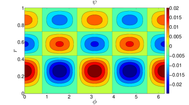
Figure 1: Streamfunction of the primary wave $\psi_{w}$ for $n_{p}=2$, with an arbitrary amplitude for illustration. Contours of constant $\psi_{w}$ are the streamlines of the primary wave flow. The flow goes clockwise around the red streamlines and anticlockwise around the blue streamlines. Stagnation points are located at the radial nodes $r$ where $J_{2}(kr)=0$, at azimuthal locations $\phi=\frac{(2n+1)}{4}\pi$ for $n\in\mathbb{Z}$.

This wave overturns the stratification when $\partial_{r}s<0$, where $s=(1/2)r^{2}+b_{w}$ is proportional to the total entropy. This is equivalent to $\frac{1}{r}\partial_{r}b_{w}<-1$. Note that overturning occurs only when $A>1$, and is more likely for waves with large radial node numbers and small azimuthal wavenumbers. The size of the convectively unstable region of the $m=2$ primary wave can be illustrated for a given $A$ and $n_{p}$, by calculating

$$N^{2} = g\partial_{r}s=r(r+\partial_{r}b)$$

$$= r^{2}+\frac{2A}{k}r\left(J_{1}(kr)-J_{3}(kr)\right)\cos 2\phi.$$

For illustration, we plot the 2D region that is convectively unstable for several $A$ values when $n_{p}=2$ in Fig. 2. An approximate size for the overturning region for small $r$ when $A>1$ is

$$r_{ov}\approx\sqrt{\frac{6}{k^{2}}\left(1-\frac{1}{A}\right)},$$ (18)

at the most unstable wave phase. When $A=1$ the overturning region is the point $r=0$, with the region expanding for larger $A$. If the instabilities that cause wave breaking are convectively driven, we would expect them to be strongly (though not necessarily completely) localised within these convectively unstable regions of the primary wave.

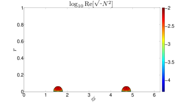
Figure 2: Spatial exent of the region that is made convectively unstable by the primary wave for $A=1.1$ (top) and $10$ (bottom), with $n_{p}=2$. This region expands from the point $r=0$ when $A=1$ to encompass the innermost few wavelengths for larger $A$.

2.2 Infinitesimal perturbations

We consider linear perturbations to this finite-amplitude primary wave, which we expand as (dropping the primes from now on)

$$\psi = \sum_{m=-\infty}^{\infty}\sum_{n=0}^{\infty}\psi_{m,n}(t)J_{m}(k_{m,n}r)e^{im\phi},$$ (19)

$$b = \sum_{m=-\infty}^{\infty}\sum_{n=0}^{\infty}b_{m,n}(t)J_{m}(k_{m,n}r)e^{im\phi},$$ (20)

where $k_{m,n}$ is chosen such that the solutions for each azimuthal wavenumber $m$, and radial node number $n\geq 0$, satisfy the outer boundary condition at $r=1$, for which

$$J_{m}(k_{m,n})=0.$$ (21)

This condition forces $k_{m,n}\in\mathbb{R}$, for $|m|,n\in\mathbb{Z}^{+}$. The above expansion automatically enforces a regularity condition on the perturbations at $r=0$. Eqs. 19 and 20 define our Galerkin basis. This basis is adopted for two reasons: the linear solutions ($A=0$) take the same form, and it automatically satisfies the chosen boundary conditions.

Note that our spectral-space amplitudes $\psi_{m,n}(t),b_{m,n}(t)\in\mathbb{C}$, so we must take the real part at the end of the calculation to obtain physical quantities. For each $m$, there is an infinite number of components with different values of $n$. In our spectral representation of the solution, we truncate these infinite series such that $1-L_{m}\leq m\leq L_{m}-1$, where $L_{m}$ is an odd number, and $0\leq n\leq L_{n}$. This truncation is chosen so that we have an exactly equal number either side of $m=0$ (and a similar number either side of the primary wave $m=2$) which ensures that our mathematical realisation of the problem has the symmetry property that we discuss in § 5.3 below.

2.3 Derivation of the evolutionary equations

Evolutionary equations for the amplitudes $\psi_{m,n}(t)$ and $b_{m,n}(t)$ can be derived by projection through integration onto the Galerkin basis. To do this we substitute the above expansions into the linear system defined by Eqs. 14–15. An important orthogonality relation is

$$\int_{0}^{2\pi}\int_{0}^{1}rJ_{m^{\prime}}(k_{m^{\prime},n^{\prime}}r)J_{m}(k_{m,n}r)e^{i(m-m^{\prime})\phi}drd\phi$$

$$\hskip 78.24507pt=\pi\left[J_{m+1}(k_{m,n})\right]^{2}\delta_{n,n^{\prime}}\delta_{m,m^{\prime}},$$ (22)

where $\delta$ is the Kronecker delta. Note that this results in different normalisation factors for each $m$ and $n$ wave. Also note that

$$-\nabla^{2}\left(J_{m}(k_{m,n}r)e^{im\phi}\right)=k_{m,n}^{2}J_{m}(k_{m,n}r)e^{im\phi}.$$ (23)

2.4 Linear solutions (in the absence of the primary wave)

Consider Eqs. 14–15 with $J(\dots,\dots)=0$, which is equivalent to having a hydrostatic background with no primary wave flow. If we substitute the expansions Eq. 19–20 into Eqs. 14–15, and then multiply by $rJ_{m^{\prime}}(k_{m^{\prime}n^{\prime}}r)e^{-im^{\prime}\phi}$, and finally integrate over $\phi\in[0,2\pi]$ and $r\in[0,1]$, we obtain

$$k_{m,n}^{2}\dot{\psi}_{m,n}+imb_{m,n}=0$$ (24)

$$\dot{b}_{m,n}+im\psi_{m,n}=0$$ (25)

for each $m,n$, after relabelling $m^{\prime}\rightarrow m$, and $n^{\prime}\rightarrow n$ following the integration. This system, together with the boundary conditions, can be solved to give

$$\psi_{m,n}=A_{m,n}e^{-i\omega_{m,n}t}+B_{m,n}e^{i\omega_{m,n}t},$$ (26)

with $A_{m,n},B_{m,n}\in\mathbb{C}$, and $\omega_{m,n}=\pm m/k_{m,n}$. This is the frequency of a non-interacting wave which is able to exist in the container in the absence of any primary wave flow. If we do not truncate the Galerkin basis at some finite values of $L_{n}$ and $L_{m}$, then these modes would be dense in the frequency interval $(0,1)$, since the maximum buoyancy frequency $N_{max}=1$. In a frame in which the fluid rotates with angular velocity $\Omega$, the Doppler-shifted wave frequency is $\hat{\omega}_{m,n}=\omega_{m,n}-m\Omega$. Note that $k_{m,n}$ increases with both $m$ and $n$, but $\omega_{m,n}$ decreases with $n$ and increases with $m$. When substituting the above solution back into Eq. 19–20, we obtain the linear solutions of the system, which are Bessel functions of a given order $|m|$ with $n$ nodes in the radial direction. This motivated our choice of Galerkin basis.

2.5 Nonlinear terms

We obtain our system of equations from Eqs. 14–15 through the same approach as in the previous section, to obtain for each $m$ and $n$,

$$k_{m,n}^{2}\dot{\psi}_{m,n}+imb_{m,n} = \frac{1}{\pi\left[J_{m+1}(k_{m,n})\right]^{2}}\int_{0}^{2\pi}\int_{0}^{1}$$ (27)

$$\bigg{\{}rJ_{m}(k_{m,n}r)e^{-im\phi}\left[J(\psi_{w},-\nabla^{2}\psi)\right.$$

$$\left.+J(\psi,-\nabla^{2}\psi_{w})\right]\bigg{\}}drd\phi,$$

$$\dot{b}_{m,n}+im\psi_{m,n} = \frac{1}{\pi\left[J_{m+1}(k_{m,n})\right]^{2}}\int_{0}^{2\pi}\int_{0}^{1}$$ (28)

$$\bigg{\{}rJ_{m}(k_{m,n}r)e^{-im\phi}\left[J(\psi_{w},b)\right.$$

$$\left.+J(\psi,b_{w})\right]\bigg{\}}drd\phi,$$

where the Jacobians contain sums over $n^{\prime}$ and $m^{\prime}$. The sum over $m^{\prime}$ is reduced to a pair of terms through the $\phi$ integration, using Eq. 2.3. A set of coupling integrals of triple products of Bessel functions also results, for which there is a sum of such terms over $n^{\prime}$, i.e., an $m,n$ wave is coupled through nonlinear terms to waves with $m\pm 2$ and (in principle) all node numbers $n\in\{0,\dots,\infty\}$. The system reduces to

$$k_{m,n}^{2}\dot{\psi}_{m,n}+imb_{m,n} = \sum_{n^{\prime}=0}^{\infty}\bigg{\{}i\alpha_{m,n,n^{\prime}}\left(k_{m-2,n^{\prime}}^{2}-k_{2,n_{p}}^{2}\right)\tilde{A}\psi_{m-2,n^{\prime}}$$ (29)

$$+i\beta_{m,n,n^{\prime}}\left(k_{m+2,n^{\prime}}^{2}-k_{2,n_{p}}^{2}\right)\tilde{A}^{*}\psi_{m+2,n^{\prime}}\bigg{\}},$$

$$\dot{b}_{m,n}+im\psi_{m,n} = \sum_{n^{\prime}=0}^{\infty}\bigg{\{}i\alpha_{m,n,n^{\prime}}\tilde{A}\left(b_{m-2,n^{\prime}}-k_{2,n_{p}}\psi_{m-2,n^{\prime}}\right)$$ (30)

$$+i\beta_{m,n,n^{\prime}}\tilde{A}^{*}\left(b_{m+2,n^{\prime}}-k_{2,n_{p}}\psi_{m+2,n^{\prime}}\right)\bigg{\}},$$

where

$$\tilde{A}=\frac{2}{k_{2,n_{p}}^{3}}A.$$ (31)

The coupling coefficients are

$$\alpha_{m,n,n^{\prime}} = \underbrace{\frac{2}{\left[J_{m+1}(k_{m,n})\right]^{2}}}_{\mathrm{normalisation}}\left((m-2)\mathcal{I}^{1}_{m,n,n^{\prime}}-2\mathcal{I}^{2}_{m,n,n^{\prime}}\right),$$ (32)

$$\beta_{m,n,n^{\prime}} = \underbrace{\frac{2}{\left[J_{m+1}(k_{m,n})\right]^{2}}}_{\mathrm{normalisation}}\left((m+2)\mathcal{I}^{3}_{m,n,n^{\prime}}+2\mathcal{I}^{4}_{m,n,n^{\prime}}\right),$$ (33)

with the integrals

$$\mathcal{I}^{1}_{m,n,n^{\prime}} = \int_{0}^{1}J_{m}(k_{m,n}r)\left[\partial_{r}J_{2}(k_{2,n_{p}}r)\right]J_{m-2}(k_{m-2,n^{\prime}}r)dr,$$

$$\mathcal{I}^{2}_{m,n,n^{\prime}} = \int_{0}^{1}J_{m}(k_{m,n}r)J_{2}(k_{2,n_{p}}r)\left[\partial_{r}J_{m-2}(k_{m-2,n^{\prime}}r)\right]dr,$$

$$\mathcal{I}^{3}_{m,n,n^{\prime}} = \int_{0}^{1}J_{m}(k_{m,n}r)\left[\partial_{r}J_{2}(k_{2,n_{p}}r)\right]J_{m+2}(k_{m+2,n^{\prime}}r)dr,$$

$$\mathcal{I}^{4}_{m,n,n^{\prime}} = \int_{0}^{1}J_{m}(k_{m,n}r)J_{2}(k_{2,n_{p}}r)\left[\partial_{r}J_{m+2}(k_{m+2,n^{\prime}}r)\right]dr.$$

Note that these are related by

$$\mathcal{I}^{3}_{m,n,n^{\prime}} = \mathcal{I}^{1}_{m+2,n^{\prime},n}\;,$$ (34)

$$\mathcal{I}^{4}_{m,n,n^{\prime}} = \mathcal{I}^{2}_{m+2,n^{\prime},n}-\mathcal{I}^{1}_{m+2,n^{\prime},n}\;,$$ (35)

where the latter follows from an integration by parts. For use in the derivation of the spectral space energy equation in a subsequent section, we find it convenient to define

$$\tilde{\alpha}_{m,n,n^{\prime}}=\pi\left[J_{m+1}(k_{m,n})\right]^{2}\alpha_{m,n,n^{\prime}},$$ (36)

and similarly for $\tilde{\beta}_{m,n,n^{\prime}}$. This is because we then have the relation

$$\tilde{\beta}_{m,n,n^{\prime}}=\tilde{\alpha}_{m+2,n^{\prime},n}.$$ (37)

2.6 Diffusive terms

In the presence of viscosity and radiative diffusion (or hyperdiffusion) Eqs. 14 and 15 have the additional terms $(-1)^{2+\alpha}\nu\nabla^{2+2\alpha}\psi$ and $(-1)^{1+\alpha}\kappa\nabla^{2\alpha}b$, respectively. Here $\alpha$ is chosen to give the standard diffusive operator ($\alpha=1$), or hyperdiffusion ($\alpha=2,3$). In this case we obtain the (linearised) system

$$k_{m,n}^{2}\dot{\psi}_{m,n}+imb_{m,n}=-\nu k_{m,n}^{2+2\alpha}\psi_{m,n},$$ (38)

$$\dot{b}_{m,n}+im\psi_{m,n}=-\kappa k_{m,n}^{2\alpha}b_{m,n},$$ (39)

instead of Eqs. 24–25, where $\nu$ is the kinematic (hyper-) viscosity and $\kappa$ is the thermal (hyper-) diffusivity, with similar modifications to Eqs. 29–30. The dispersion relation is then

$$\left(\omega_{m,n}+i\nu k_{m,n}^{2\alpha}\right)\left(\omega_{m,n}+i\kappa k_{m,n}^{2\alpha}\right)=\frac{m^{2}}{k_{m,n}^{2}},$$ (40)

indicating that the frequencies of the allowed solutions are modified in the presence of $\nu,\kappa$. The growth rate expected in the presence of weak diffusion is therefore $\mathrm{Im}\left[\omega\right]-\frac{1}{2}(\nu+\kappa)k_{m,n}^{2\alpha}$, with $\mathrm{Im}\left[\omega\right]$ being the appropriate inviscid growth rate. Since Eqs. 29–30 allow instability, to obtain growing modes in the presence of diffusion, $\nu$ and $\kappa$ must be sufficiently weak so that diffusive terms do not dominate over the nonlinear terms except for values of $n$ and $m$ close to the resolution limits of $L_{n}$ and $L_{m}$. Hyperdiffusion with $\alpha=3$ is adopted since it better restricts the dissipation to the highest wavenumbers. This enables numerical convergence in the eigenvalue problem discussed below, but does not significantly perturb the growth rates of the lower wavenumber eigenmodes with the values of $\nu,\kappa$ that we adopt. From here on, we also take $\nu=\kappa$.

With the inclusion of diffusive terms we require $1+2\alpha$ additional boundary conditions at each boundary. These are regularity conditions at the centre, and at the outer boundary we can consider a variety of idealised boundary conditions of the form $\nabla^{2\sigma}\psi=0$ for $\sigma=0,1,\dots,\alpha$ and $\nabla^{2\sigma}b=0$ for $\sigma=0,1,\dots,\alpha-1$. These are automatically satisfied by our Galerkin basis Eq. 19–20 and the definition of $k_{m,n}$. With these boundary conditions (which force $k_{m,n}$ to be real), the Galerkin basis is therefore exact for the single-wave diffusive problem. Note that this is also true if hyperdiffusion is adopted, due to property Eq. 23. In the numerical solution of the eigenvalue problem in the following sections we include these diffusive terms to achieve numerical convergence. This is necessary because in the absence of diffusion, the most unstable modes are found to prefer the smallest spatial scales.

3 Method of solution

Our system Eqs. 27–28 can be written in the form of a generalised eigenvalue problem of the form

$$\boldsymbol{\mathrm{A}}\mathbf{U}=\omega\boldsymbol{\mathrm{B}}\mathbf{U},$$ (41)

where $\mathbf{U}$ is the column vector whose components are the quantities $(\psi_{m,n},b_{m,n})$ for each $m$ and $n$. $\boldsymbol{\mathrm{A}}$ is the block tridiagonal matrix representing the system. This is done by seeking normal mode solutions of the form $\psi_{m,n}(t)\propto e^{-i\omega t}$ for each $m$ and $n$, and similarly for $b_{m,n}(t)$. $\boldsymbol{\mathrm{B}}$ is the diagonal matrix that can be composed as blocks of the form

$$-i\left(\begin{array}[]{cc}k_{m,n}^{2}&0\\ 0&1\\ \end{array}\right),$$ (44)

for each $m$ and $n$. We solve this problem using standard generalised eigenvalue solver routines, such as ZGGEV in the LAPACK library. This returns the eigenvalues $\{\omega\}$, and the spectral space eigenfunctions $\{\psi_{m,n},b_{m,n}\}$ corresponding to each eigenvalue. The real space eigenfunctions can be reconstructed from these, using Eqs. 19–20.

We choose $L_{n}=50$ and $L_{m}=27$ for most of the calculations (though a small number of higher resolution calculations were performed with $L_{m}$ values up to $45$, which confirm that our results are not dependent on resolution). There is a limit to the maximum values of $L_{n}$ and $L_{m}$ that we can reasonably adopt, due to the computational cost of choosing large values for each of these parameters. One reason for this is that the nonlinear terms require the computation of a large number of integrals, many of which have highly oscillatory integrands, and require very small relative error tolerances to be computed accurately (by the method of computation that we will describe in the next subsection). Another reason is that we compute the eigenvalues and eigenvectors using a QZ alogorithm, which has a high computational cost $O(10S^{3})$ for an $S\times S$ matrix, where $S=2L_{m}\left(L_{n}-1\right)$. This limits the values of $L_{n}$ and $L_{m}$. With our choice of $\alpha=3$ hyperdiffusion, it has been found that $10^{-14}\leq\nu\leq 10^{-11}$ is appropriate. This hyperdiffusion is found to give the spurious eigenvalues, whose eigenfunctions oscillate at the smallest scales, and are therefore not adequately resolved, a large decay rate, and allows our growing modes to be adequately converged for the values of $A$ and $n_{p}$ that we consider.

3.1 Numerical computation of table of integrals

The tables of integrals defined in § 2.5 are computed for each value of $m,n,n^{\prime}$ using a 4th/5th order adaptive step Runge-Kutta integrator. To enable efficient computations, the Bessel functions are computed simultaneously with the integrals. Note that Bessel’s equation

$$\partial_{r}(r\partial_{r}\psi)+r\left(k_{m,n}^{2}-\frac{m^{2}}{r^{2}}\right)\psi=0,$$ (45)

can be rewritten as the coupled set of first order ODEs

$$\frac{d\xi}{dr} = r\left(\frac{m^{2}}{r^{2}}-k_{m,n}^{2}\right)\psi,$$ (46)

$$\frac{d\psi}{dr} = \frac{\xi}{r}.$$ (47)

We also need the derivatives of various Bessel functions, so we also integrate

$$\frac{d^{2}\psi}{dr^{2}}=\frac{(m^{2}-r^{2}k_{m,n}^{2})\psi-\xi}{r^{2}},$$ (48)

to obtain the first derivative of each Bessel function. To compute the integrals, we integrate the integrands of $\mathcal{I}^{i}_{m,n,n^{\prime}}$ for $i\in\{1,2,3,4\}$, and take the value at $r=1$. This involves solving a system of 15 ODEs in total for each $m,n,n^{\prime}$. Using our chosen resolution of $L_{n}=50$, $L_{m}=27$, this involves the computation of $L_{m}(L_{n}-1)^{2}\sim 10^{5}$ integrals in total. These are computed for a given number of radial nodes in the primary wave in the range $0\leq n_{p}\leq 12$. We impose an inner boundary at $r_{in}=10^{-4}$ to avoid the coordinate singularity at the origin, and use initial conditions appropriate from considering the asymptotic behaviour of the Bessel functions. For small $L_{n}$ and $L_{m}$ values the numerical integrals have been checked to agree with those computed from Mathematica, and for large $L_{n}$ and $L_{m}$, several integrals containing the highest $n$ and $m$ values were also checked. We use a relative error tolerance of $10^{-13}$, which has been found to compute the most oscillatory integrals (corresponding to the highest $n$ and $m$ value) accurately (compared with Mathematica) to within at least $6$ decimal places.

4 Kinetic and potential energy equations

The kinetic and potential energies can be computed from either the real-space or spectral-space eigenfunctions. This enables a determination of the dominant source of free energy driving the instability (e.g. Lombard & Riley 1996), and also provides an independent calculation of the growth rate, which can be used to check our numerical code. We derive an energy equation in spectral space, and compute the volume-integrated terms using the numerically computed eigenfunctions, without converting to real space. This has been found to reduce numerical errors, resulting from large numerical cancellations in the most oscillatory Bessel functions, when the energy equations are instead computed in real space. In addition, it is simpler to construct the (hyper-) diffusion terms in spectral space, so that they can be fully taken into account in the energy budget.

We define

$$K = \int_{0}^{2\pi}\int_{0}^{1}\frac{1}{2}|\mathbf{u}|^{2}rdrd\phi,$$ (49)

$$P = \int_{0}^{2\pi}\int_{0}^{1}\frac{1}{2}b^{2}rdrd\phi,$$ (50)

$$E = K+P,$$ (51)

as the kinetic, potential and total energy densities of the disturbance, respectively. Note that

$$K = \frac{1}{2}\sum_{m=-\infty}^{\infty}\sum_{n=0}^{\infty}k_{m,n}^{2}|\psi_{m,n}|^{2}\pi\left[J_{m+1}(k_{m,n})\right]^{2},$$ (52)

$$P = \frac{1}{2}\sum_{m=-\infty}^{\infty}\sum_{n=0}^{\infty}|b_{m,n}|^{2}\pi\left[J_{m+1}(k_{m,n})\right]^{2},$$ (53)

$$E = K+P.$$ (54)

Evolutionary equations for the volume-integrated energy can be obtained from Eq. 29 and 30 together with the (hyper-) diffusion terms. After some rearrangement, these can be written

$$\dot{K} = \mathcal{N}_{sw}+F_{b}+F_{\nu},$$ (55)

$$\dot{P} = \mathcal{N}_{bw}-F_{b}+F_{\kappa},$$ (56)

$$\dot{E} = \mathcal{N}_{sw}+\mathcal{N}_{bw}+F_{\nu}+F_{\kappa},$$ (57)

where

$$\mathcal{N}_{sw} = \mathrm{Re}\sum_{m=-\infty}^{\infty}\sum_{n=0}^{\infty}\sum_{n^{\prime}=0}^{\infty}i\tilde{\alpha}_{m,n,n^{\prime}}\left(k_{m-2,n^{\prime}}^{2}-k_{m,n^{\prime}}^{2}\right)$$

$$\hskip 113.81102pt\tilde{A}\psi_{m,n}^{*}\psi_{m-2,n^{\prime}},$$

$$\mathcal{N}_{bw} = \mathrm{Re}\sum_{m=-\infty}^{\infty}\sum_{n=0}^{\infty}\sum_{n^{\prime}=0}^{\infty}i\tilde{\alpha}_{m,n,n^{\prime}}\tilde{A}k_{2,n_{p}}$$

$$\hskip 56.9055pt\left(b_{m,n}^{*}\psi_{m-2,n^{\prime}}+\psi_{m,n}^{*}b_{m-2,n^{\prime}}\right),$$

$$F_{b} = \mathrm{Re}\sum_{m=-\infty}^{\infty}\sum_{n=0}^{\infty}im\psi_{m,n}^{*}b_{m,n}\pi\left[J_{m+1}(k_{m,n})\right]^{2},$$

$$F_{\nu} = \mathrm{Re}\sum_{m=-\infty}^{\infty}\sum_{n=0}^{\infty}-\nu k_{m,n}^{2+2\alpha}|\psi_{m,n}|^{2}\pi\left[J_{m+1}(k_{m,n})\right]^{2},$$

$$F_{\kappa} = \mathrm{Re}\sum_{m=-\infty}^{\infty}\sum_{n=0}^{\infty}-\kappa k_{m,n}^{2\alpha}|b_{m,n}|^{2}\pi\left[J_{m+1}(k_{m,n})\right]^{2}.$$

$\mathcal{N}_{sw}$ represents the production of perturbation kinetic energy from the primary wave shear. $\mathcal{N}_{bw}$ represents the production of perturbation potential energy from the primary wave entropy gradients. Whichever of $\mathcal{N}_{sw}$ or $\mathcal{N}_{bw}$ is dominant tells us whether this instability is driven by the wave shear or the wave entropy gradients. $F_{b}$ is the buoyancy flux term, representing conversion between kinetic and potential energies of the disturbance. Finally, $F_{\nu}$ and $F_{\kappa}$ represent the irreversible loss of kinetic and potential energies as a result of the (hyper-) diffusion.

After truncation at $|m|=L_{m}$ and $n=n^{\prime}=L_{n}$, each of these terms are computed from the spectral space eigenfunctions, together with the numerically computed table of integrals. The growth rate can then be computed from

$$\mathrm{Im}[\omega{{}^{\prime}}]=\frac{\dot{E}}{2E}=\frac{\dot{K}}{2K}=\frac{\dot{P}}{2P}.$$ (58)

We have checked that each of these equations are accurately satisfied to within at worst a few percent for each of the unstable modes discussed in this paper. This provides a check of our analytical derivations and numerical calculations, and should convince ourselves that our results are consistent.

5 Numerical tests

In this section we briefly mention several numerical tests which we have performed to validate our numerical code, in addition to the one mentioned in the previous section. Following this section, in § 6 and 7 we discuss the results of our stability analysis for waves with $A<1$ and $A>1$, respectively.

5.1 Linear

In the absence of nonlinear couplings ($A=0$), we obtain a set of non-interacting modes with eigenfreqencies $\omega\in\{\omega_{m,n}\}$, where $\omega_{m,n}=\pm m/k_{m,n}$ (in the inertial frame), as we predicted in § 2.4. In the absence of diffusion, these have zero growth rate, i.e., Im$\left[\omega\right]=0$, for all eigenmodes. When hyperdiffusion is included, the eigenmodes each have a nonzero decay rate determined by the values of $\nu$ and $\kappa$, which is very accurately (to more than 10 decimal places) computed from considering only the terms $F_{\nu}$ and $F_{\kappa}$ in the energy equation. The real-space eigenfunctions that result are what is predicted from linear theory, in that they are Bessel functions of order $m$ with $n$ nodes in the radial direction.

5.2 Weakly nonlinear

We followed a typical eigenmode as $A$ is gradually increased from zero, and found that for $|A|\ll 1$, the shift in the eigenfrequency $\mathrm{Re}[\delta\omega]\propto A^{2}$, as we would expect for modes not undergoing parametric resonance (e.g. Landau & Lifshitz 1969).

5.3 Symmetries

The real-space solutions can be represented in the form

$$\mathrm{Re}\left[\sum_{m}\sum_{n}c_{m,n}(r)e^{i(m\phi-\omega t)}\right].$$ (59)

This is symmetric under the transformations $c_{m,n}(r)\rightarrow c_{m.n}^{*}(r)$, $m\rightarrow-m$ and $\omega\rightarrow-\omega^{*}$. This symmetry should exist for all primary wave amplitudes, and results from the fact that only the sign of the pattern speed $\omega/m$ has meaning, and not the sign of the wavenumber or frequency. This means that when the eigenvalues are plotted on the complex frequency plane, they should be symmetric about $\mathrm{Re}\left[\omega\right]=0$.

6 Results for waves with $A<1$: parametric instabilities

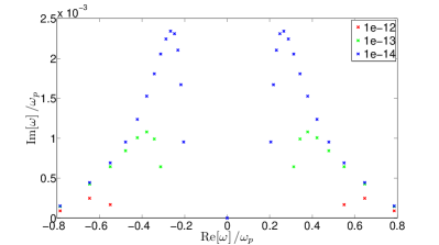
Figure 3: Distribution of unstable eigenvalues on the complex frequency plane for $A=0.1$, $n_{p}=2$ and $\nu=10^{-12},10^{-13},10^{-14}$.

We examine the unstable modes that exist when $0<A<1$, which is when the primary wave does not overturn the stratification at any location in the wave. The instability is a parametric instability, for which a simple model is briefly reviewed in Appendix A. When $A\neq 0$, the fraction of eigenmodes that are growing is nonzero (above a critical $A$ set by the values of $n_{p}$ and $\nu$, which can be understood from Eq. 75) and increases with $A$, as nonlinear growth starts to dominate over the decay due to diffusion for a larger number of modes. For small $A$, the eigenvalues of the unstable modes displayed on the complex plane are distributed in two curves which are symmetric about $\mathrm{Re}\left[\omega\right]=0$. This is illustrated in Fig. 3, and is a result of the symmetry described in § 5.3.

In the limit that $A\rightarrow 0$, the unstable modes can be identified as the parametrically excited free-wave modes. These are a pair of free wave modes that exist when $A=0$, which undergo modifications to their complex frequencies at $O(A)$ that reinforce each other. We have verified that the modes consist of a pair whose frequencies approximately add up to $\omega_{p}$ in the inertial frame, with a detuning $\Delta/\omega_{p}\lesssim 10^{-2}$. As $A$ is increased, the unstable modes consist of gradually more complicated superpositions of free wave modes, until for $A\gtrsim 1$, the eigenfunctions become localised in the convectively unstable regions. This will be studied in more detail in § 7. For $A\lesssim 1$, the eigenfunctions exist because of their confinement by the boundaries, though they interact quite strongly with the primary wave, and are generally not simply free wave modes with a nonzero growth rate.

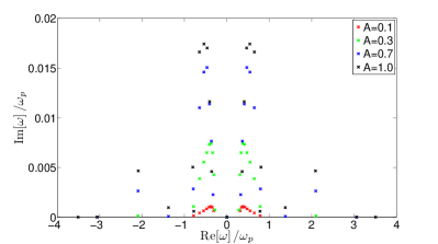
Figure 4: Distribution of unstable eigenvalues on the complex frequency plane for various values of $A$, with $n_{p}=2$ and $\nu=10^{-14}$.

The number of unstable modes that exist in this amplitude range depends quite strongly on viscosity. This is illustrated in Fig. 3. The number is also found to decrease as $n_{p}$ is increased. These two behaviours are related by the fact the a wave should undergo parametric instabilities, which have largest growth rates when the resonant tuning is good, which is more likely to occur for perturbations with larger wavenumbers. However, these large wavenumber components are strongly damped by diffusion. Increasing $n_{p}$ means that the “effective resolution” available to capture the unstable modes decreases. This is the same as increasing $\nu$, hence the same trends exhibited in increasing $n_{p}$ and $\nu$.

The neat distribution of eigenvalues into two curves does not persist as $A$ is increased, as illustrated in Fig. 4. The frequencies (in the rotating frame) are primarily smaller than the primary wave frequency in the inertial frame. However, a small number of modes exist for $A\gtrsim 0.3$ which have frequencies larger than $\omega_{p}$. Nevertheless, in each case the frequencies of the unstable modes are always smaller than the maximum buoyancy frequency in the flow (which corresponds with $1/\omega_{p}\sim 6$ in the units of this figure, for $n_{p}=2$). This makes sense if these are gravity wave-like disturbances, which are parametrically excited by the primary wave.

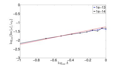
Figure 5: Im$\left[\omega\right]$ vs. $A$ for the most unstable mode with $n_{p}=2$ and $\nu=10^{-13},10^{-14}$. The solid red line has slope $1$. This shows that the instability approximately scales linearly with $A$ for small $A$, indicating that the instability when $A<1$ is due to a parametric resonance.

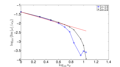
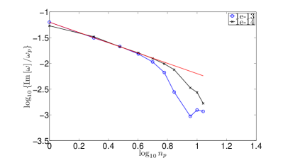
Figure 6: $\log_{10}$Im$\left[\omega/\omega_{p}\right]$ vs. $\log_{10}n_{p}$ for the most unstable mode when $A=0.5$ and $0.8$ respectively, for $\nu=10^{-13}$ and $10^{-14}$. The red line has a slope $-1$. The tail-off at larger $n_{p}$ is due to diffusion.

In Fig. 5, the growth rate for the most unstable mode is shown to scale approximately linearly with $A$ for $A\leq 1$. A slope of $1$ in this figure is predicted for $A\ll 1$ if the instability is due to a parametric resonance, and this appears to approximately hold for all $A$ in this range.

Our most important result of this study is illustrated in Fig. 6. This shows that the growth rate scales inversely with the number of wavelengths within the domain (note that this is after normalising by $\omega_{p}$). In this figure we plot the logarithm of the growth rate versus $\log_{10}n_{p}$ for $A=0.5$ and $0.8$, respectively. The slope is always approximately equal to $-1$ for low $n_{p}$. The tail-off at larger $n_{p}$ is due to diffusion, and arises because modes with smaller spatial scales parametrically excite modes with even smaller spatial scales (as a result of the theorem proved by Hasselmann 1967), which are then more easily damped by diffusion. As we would expect from this interpretation, the value of $n_{p}$ at which diffusion dominates moves to smaller $n_{p}$ as $\nu$ is increased. The inverse dependence on $n_{p}$ that is present when diffusion is unimportant is a key result. This suggests that although parametric instabilities exist for any amplitude in the absence of diffusion, in a sufficiently large domain they become unimportant. We discuss the relevance of this result to tidal dissipation in § 8.

6.1 Eigenfunctions

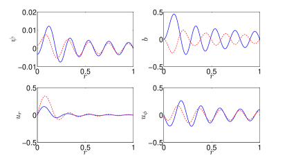
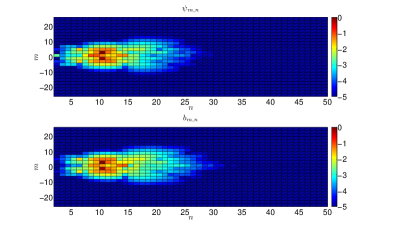
Figure 7: Top: Real (blue solid lines) and imaginary (red dashed lines) parts along $\phi=0$ of the spatial eigenfunctions for the most unstable mode for $A=0.1$, $n_{p}=2$, $\nu=10^{-13}$. The eigenfrequency is $\omega/\omega_{p}=0.378+0.001i$. Bottom: Spectral space eigenfunction of the same mode. The colour scale represents $\log_{10}|\psi_{m,n}/\mathrm{max}\{\psi_{m,n}\}|$, and similarly for $b_{m,n}$.

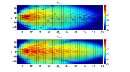
Figure 8: Top: Real (blue solid lines) and imaginary (red dashed lines) parts along $\phi=0$ of the spatial eigenfunctions for the most unstable mode with $A=1$, $n_{p}=2$, $\nu=10^{-13}$. The eigenfrequency is $\omega/\omega_{p}=0.540+0.017i$. Bottom: Spectral space eigenfunction of the same mode. The colour scale represents $\log_{10}|\psi_{m,n}/\mathrm{max}\{\psi_{m,n}\}|$, and similarly for $b_{m,n}$.

In the top panels of Figs. 7 and 8 we plot the real (blue solid lines) and imaginary parts (red dashed lines) along $\phi=0$ of the spatial eigenfunctions of the most unstable mode for $A=0.1$ and $0.5$, respectively. We have taken $n_{p}=2$ and $\nu=10^{-13}$. These modes exist throughout the box and are confined by the boundary. They become more distorted from the free wave modes as $A$ is increased towards unity (and in fact also for $A>1$, apart from the localised modes), especially in the innermost wavelengths of the primary wave. Note that the amplitude of the eigenfunctions is arbitrary since we are solving an eigenvalue problem. The bottom panels of Figs. 7 and 8 show the spectral space eigenfunctions of the same unstable modes. We have normalised $\psi_{m,n}$ and $b_{m,n}$ to their maximum values and taken the base 10 logarithm of each component to produce the figures. These show that growing modes for the chosen values of $A$ are not simply a pair of free wave modes which are excited by the primary wave. They contain many $n$ and $m$ values localised around a particular $n$ and $m$, and are therefore interacting strongly with the primary wave. Multiple $n$ and $m$ values are involved even when $A=0.1$. For the value of $\nu$ adopted, these modes are well resolved, as is shown from the amplitude decay of the spectral space eigenfunction, which occurs before the resolution limit is reached in $n$ and $m$.

6.2 Energetics of the instabilities

When $A<1$, the isentropes are never overturned by the primary wave, so a pure radial convective instability is not possible. However, these instabilities could be driven by the free energy resulting from the primary wave shear or entropy gradients, or a combination of the two. In this section, we compute the spectral-space energy contributions outlined in § 4, for a sample of growing modes in this amplitude range. We have confirmed that the growth rate is accurately computed from Eq. 58, to within a few percent at most. In Table 1 we outline the contributions to the growth rate from each term in Eqs. 55–57 for the most unstable mode for $A=0.1,0.5$ and $1$ with $n_{p}=2$ and $\nu=10^{-13}$. The eigenfunctions for two of these are plotted in Figs. 7 and 8. These examples are illustrative of every unstable mode that exists when $A<1$ (and also the non-localised modes that exist when $A>1$).

	$A=0.1$	$A=0.5$	$A=1$
$\mathrm{Re}\left[\omega\right]$	$0.065$	$0.080$	$0.093$
$\mathrm{Im}\left[\omega\right]$	$1.86\times 10^{-4}$	$1.97\times 10^{-3}$	$3.00\times 10^{-3}$
$K$	$3.28\times 10^{-2}$	$3.82\times 10^{-2}$	$3.70\times 10^{-2}$
$P$	$3.25\times 10^{-2}$	$3.87\times 10^{-2}$	$4.16\times 10^{-2}$
$\mathcal{N}_{sw}$	$-3.20\times 10^{-7}$	$-3.98\times 10^{-5}$	$-9.55\times 10^{-5}$
$\mathcal{N}_{bw}$	$3.57\times 10^{-5}$	$3.76\times 10^{-4}$	$6.62\times 10^{-4}$
$F_{b}$	$1.81\times 10^{-5}$	$2.04\times 10^{-4}$	$3.51\times 10^{-4}$
$F_{\nu}$	$-5.58\times 10^{-6}$	$-1.35\times 10^{-5}$	$-3.29\times 10^{-5}$
$F_{\kappa}$	$-5.55\times 10^{-6}$	$-2.01\times 10^{-5}$	$-6.03\times 10^{-5}$

Table 1: Energy components of the most unstable mode for $A=0.1,0.5$ and $1$, with $n_{p}=2$ and $\nu=10^{-13}$. Note that $\omega_{p}\approx 0.17$.

Firstly, we note that the integrated kinetic and potential energy of the modes are in approximate equipartition. A single wave can be proved to be in exact equipartition (as is shown in Appendix B), so we would expect $K\approx P$ if these modes are parametrically excited gravity waves with a single $n$ and $m$. That they are in approximate equipartition and include many $n$ and $m$ components indicates that these modes are the larger $A$ generalisations of the parametrically excited free wave modes. The source of free energy driving these modes is entirely the potential energy resulting from primary wave entropy gradients. Somewhat surprisingly, the primary wave shear contribution is much smaller, and actually stabilises the modes. This instability converts primary wave potential energy to disturbance potential energy, and then converts approximately half of this input energy to the disturbance kinetic energy through the buoyancy flux term. This process results in approximate equipartition between $K$ and $P$. Note that the entropy gradients in the primary wave are insufficient to cause convective instability. These modes are driven by weaker entropy gradients in radius and azimuth.

7 Results for waves with $A>1$: the initial stages of wave breaking

When $A>1$, the primary wave overturns the stratification during part of its cycle. Our simulations in BO10 have shown that an instability breaks the wave within a few wave periods once this first occurs. The initial stages of this breaking process are examined in this section by choosing $A>1$. To resolve convectively unstable modes with the adopted values of $L_{n}$ and $L_{m}$, we require the size of the overturning region to be sufficiently large. Since overturning occurs only at the point $r=0$ when $A=1$, this necessitates choosing values of $A$ larger than unity to capture such instabilities. We are interested in instabilities which act to break the waves in an (effectively) unbounded domain (the central regions of the RZ of a solar-type star), therefore the appropriate unstable mode should not rely on the boundaries for confinement, and should be localised within the innermost wavelength of the primary wave. This is because the presence of confining boundaries is artificial, and is imposed to specify the problem. With this in mind, we now discuss the results of our stability analysis for waves with $A>1$.

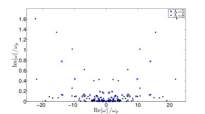
Figure 9: Distribution of unstable eigenvalues on the complex frequency plane for $n_{p}=2$ and various $A$ with $\nu=10^{-13}$.

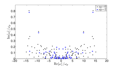
Figure 10: Distribution of unstable eigenvalues on the complex frequency plane for $A=10$ and various $n_{p}$, with $\nu=10^{-13}$.

The eigenvalues of the unstable modes displayed on the complex plane are shown in Fig. 9 for $A=5$ and $A=8$, both with $n_{p}=2$ and $\nu=10^{-13}$. The most unstable modes are located on distinct branches, which stand above the continuation of the modes that exist when $A<1$. From studying their eigenfunctions, we find that the modes on the branches are localised disturbances, unlike those below the main branches. The modes on the branches could therefore represent the type of mode that breaks the primary wave (this is discussed further in the next subsection). These branches extend further from the origin the greater the value of $A$. In Fig. 10 we plot the unstable modes for $A=5$ for two values of $n_{p}$. This shows that the unstable modes on the branches do not move around significantly as $n_{p}$ is varied. They therefore depend only weakly on the location of the outer boundary. Note, however, that the growth rate becomes smaller as we go to larger $n_{p}$ because of the increasing importance of diffusion.

Note that the largest frequency of some growing modes is larger than the maximum buoyancy frequency $N_{max}=1$ (which corresponds with $1/\omega_{p}\sim 6$ in the units of this figure, for $n_{p}=2$). The nonzero frequencies of the modes in this frame indicate that they are oscillatory, and are non-steady. In addition, the growth rates of the most unstable modes are sufficiently fast compared with the primary wave frequency that the instability grows within several wave periods after onset. This is consistent with the results of our simulations described in BO10.

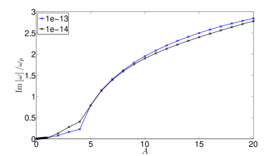
Figure 11: Im$\left[\omega\right]$ vs. $A$ for the most unstable mode for $n_{p}=2$, $\nu=10^{-13}$ and $10^{-14}$. The instability grows within a primary wave period when $A\gtrsim 5$, which is when the localised modes begin to appear.

The growth rate of the most unstable modes for a given $n_{p}$ increases with $A$ as illustrated in Fig. 11 for $n_{p}=2$, where curves for $\nu=10^{-13}$ and $10^{-14}$ have been plotted. There is an approximate square root dependence for $A\gtrsim 4$. If the instability is driven by convectively unstable entropy gradients, then we might expect

$$\mathrm{Im}\left[\omega^{\prime}\right] \lesssim \sqrt{\mathrm{max}\left[-N^{2}\right]}$$

$$= \left(\mathrm{max}\bigg{\{}-r^{2}-\frac{2A}{k_{2,n_{p}}}r\left(J_{1}(k_{2,n_{p}}r)\right.\right.$$

$$\left.\left.\hskip 71.13188pt-J_{3}(k_{2,n_{p}}r)\right)\cos 2\phi\bigg{\}}\right)^{1/2}.$$

Thus, for large $A$ the growth rate should scale with the square root of the primary wave amplitude. This behaviour is not observed when $1\lesssim A\lesssim 4$. In this range, the square root dependence may not be exhibited partly because there is insufficient resolution to accurately capture the modes that contribute to breaking since the overturning region is small compared with the box size. We have noticed that the growth rate does not significantly depend on $\nu$ (and therefore the resolution), for the most unstable modes, except in the range $1\lesssim A\lesssim 4$, which supports this explanation.

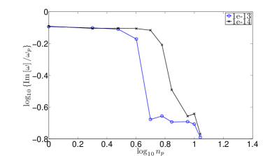
Figure 12: Im$\left[\omega\right]$ vs. $n_{p}$ for the most unstable localised modes when $A=5$ and $\nu=10^{-13}$ and $10^{-14}$.

The behaviour of the growth rate on $n_{p}$ is illustrated in Fig. 12 for the most unstable mode when $A=5$, for two values of $\nu$. For large $n_{p}$, the unstable modes have sufficiently small spatial scales for diffusion to become important, so we expect a tail-off at large $n_{p}$. The important point that can be taken from this figure is that the (normalised) growth rate of the localised modes on the branches does not depend on the number of wavelengths within the domain, for modes that are not strongly affected by diffusion. This means that the instability can be important in a large domain, such as a the RZ of a solar-type star, which contains many primary wavelengths. Note that this is very different to the behaviour found for the excited modes when $A<1$, as shown in Fig 6.

7.1 Eigenfunctions

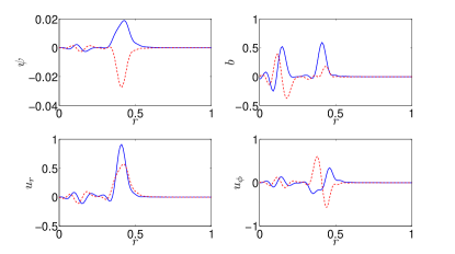
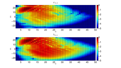
Figure 13: Top: Real (blue solid lines) and imaginary (red dashed lines) parts along $\phi=0$ of the spatial eigenfunctions for the most unstable mode with $A=5$, $n_{p}=2$, $\nu=10^{-13}$. The eigenfrequency is $\omega/\omega_{p}=9.68+0.302i$. Bottom: Spectral space eigenfunction of the same mode. The colour scale represents $\log_{10}|\psi_{m,n}/\mathrm{max}\{\psi_{m,n}\}|$, and similarly for $b_{m,n}$.

In the top panel of Fig. 13 we plot the real (blue solid lines) and imaginary parts (red dashed lines) along $\phi=0$ of the spatial eigenfunctions of the most unstable mode for $A=5$, $n_{p}=2$ and $\nu=10^{-13}$. The spectral-space eigenfunction of this mode is plotted in the bottom panel. The mode is strongly nonlinearly interacting with the primary wave, as shown by the number of different $n$ and $m$ values that appreciably contribute. The contribution to the eigenfunction is nonzero, but not maximal, near $|m|=L_{m}-1$, and is negligible at $n=L_{n}$, which indicates that this mode is adequately resolved. The eigenfunction is spatially localised within the innermost wavelengths of the primary wave. Each of the several most unstable modes in the range $5\leq A\leq 10$ which lie on the branches in Fig. 9 are localised modes, and have qualitatively different form to the type of modes that exist below the branches, which are a continuation of the modes that exist when $A<1$. As we go to larger $A$ for the same value of $\nu$, the most unstable mode utilises an increasing number of $n$ and $m$ values up to the resolution limit. This means that to adequately resolve the modes we would have to either increase the resolution or the value of $\nu$.

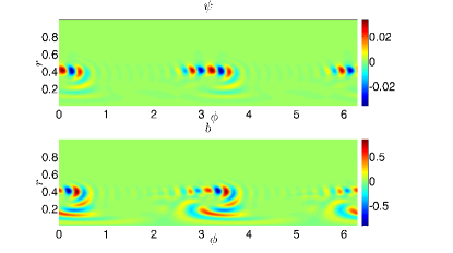
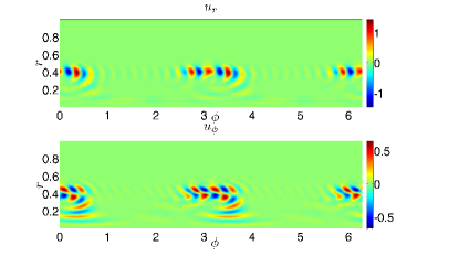
Figure 14: 2D Spatial eigenfunction of the most unstable mode for $A=10$, $n_{p}=2$ and $\nu=10^{-13}$, plotted on the $(\phi,r)$-plane.

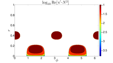
Figure 15: Unstable region for $A=10$, $n_{p}=2$. This can be compared with Fig. 14.

The components of the spatial eigenfunction of the most unstable mode when $A=5$, $n_{p}=2$ and $\nu=10^{-13}$, is plotted in Fig. 14 on the $(\phi,r)$-plane, to further illustrate the spatial dependence of this mode. In Fig. 15 we plot the region of negative $N^{2}$ for the same primary wave. A comparison of these figures makes clear that the eigenfunction is primarily localised within the regions made convectively unstable by the primary wave entropy perturbation. This adds further evidence to the conjecture that the instability is convective. We also find that any unstable mode on the branches of Fig. 9 that are excited when $5\leq A\leq 10$ are similarly localised and have a qualitatively similar appearance to the eigenfunction plotted in Fig. 14.

7.2 Energetics of the instabilities

In this section, we compute the spectral space energy contributions outlined in § 4 for a representative sample of the localised growing modes that exist when $A>1$. We have confirmed that the growth rate is accurately computed from Eq. 58, to within a few percent for the modes considered in this analysis. However, it must be noted that the most unstable mode when $A\gtrsim 5$ is typically not fully resolved with our adopted resolution and $\nu$, in that there is nonzero power in the highest $n$ and $m$ values. This can lead to errors in the energy analysis typically of order $10-30\%$, so we leave these modes out of this analysis, and only choose those that are adequately resolved for Table 2. In this table, we outline the contributions to the growth rate from each term in Eqs. 55–57 for several unstable modes that exist when $A\gtrsim 5$, each with $n_{p}=2$ and $\nu=10^{-13}$. The eigenfunction corresponding to the first of these is plotted in Figs. 13 and 14.

	$A=5$	$A=7$
$\mathrm{Re}\left[\omega\right]$	$1.67$	$2.40$
$\mathrm{Im}\left[\omega\right]$	$0.052$	$0.134$
$K$	$6.95\times 10^{-2}$	$3.37\times 10^{-2}$
$P$	$1.73\times 10^{-2}$	$1.02\times 10^{-2}$
$\mathcal{N}_{sw}$	$-5.50\times 10^{-3}$	$-1.57\times 10^{-3}$
$\mathcal{N}_{bw}$	$2.05\times 10^{-2}$	$1.55\times 10^{-2}$
$F_{b}$	$1.82\times 10^{-2}$	$1.22\times 10^{-2}$
$F_{\nu}$	$-2.10\times 10^{-3}$	$-1.33\times 10^{-3}$
$F_{\kappa}$	$-0.517\times 10^{-3}$	$-0.80\times 10^{-3}$

Table 2: Energy components of the most unstable mode for $A=5$ and $7$, with $n_{p}=2$ and $\nu=10^{-13}$. Note that $\omega_{p}\approx 0.17$.

As in the case of the modes that exist when $A<1$, the instability is driven by the free energy associated with primary wave entropy gradients, as is shown by the fact that $\mathcal{N}_{bw}$ is the dominant contribution to the growth. This is indeed what would be expected of a convectively driven instability. In addition, the primary wave shear is much weaker and tends to stabilise the modes. Unlike the modes that exist when $A<1$, we do not necessarily have $K\approx P$, and examples have been found that do and do not satisfy approximate equipartition, so these modes do not all appear to be gravity wave-like, unlike the parametrically excited modes that exist when $A<1$.

The growth rates are always $\lesssim\mathrm{Re}\left[\sqrt{-N^{2}}\right]$, which is expected to be an upper limit if the instability is convective. The negative contribution of shear, as well as hyperdiffusion mean that the modes that we have calculated have somewhat smaller growth rates that this simple estimate would predict. The route of energy transfer that drives the instability is the same as for the parametric instabilities discussed in the previous section.

8 Summary and discussion of results

In the previous two sections we have analysed the instabilities that exist when $A<1$ and $A>1$.

8.1 Wave breaking

When $A>1$ we have identified a class of localised modes that are driven by convectively unstable entropy gradients in the primary wave. These modes exist in the absence of an outer boundary, and are very likely to have initialised the wave breaking process in the simulations presented in BO10 and B11. Subsequent stages in the breaking process are not studied using this stability analysis because these would involve nonlinear interactions between the perturbations to the wave, which we neglected in our weakly nonlinear approach. The instability growth time is of the order of a primary wave period, which is in agreement with the wave breaking times observed in our simulations.

8.2 Parametric instabilities

When $A<1$, there exist pairs of parametrically excited modes driven by (convectively stable) primary wave entropy gradients, with wave shear playing a subordinate stabilising role. These modes exist because of their confinement by the outer boundary. Our most important result regarding these modes is the inverse dependence of the growth rate on $n_{p}$. This can be explained by considering the relative time the primary wave spends in the innermost regions, where its nonlinearity is strongest. The fraction of the total wave propagation time spent in the innermost regions, where growing modes are excited by the nonlinearity, scales with $k_{2,n_{p}}^{-1}\propto n_{p}^{-1}$, so the growth rate should scale also with $n_{p}^{-1}$. Combining this with our observation that the growth rate increases approximately linearly with wave amplitude, we can write

$$\mathrm{Im}\left[\omega\right]\propto\frac{A}{n_{p}},$$ (60)

for the modes excited when $A<1$.

Our simulations in BO10 and B11 did not show any instabilities acting on the waves when $A<1$. This can be neatly explained from Eq. 60 in the limit as $n_{p}\rightarrow\infty$, where the growth rate tends to zero. This limit is appropriate since the waves have effectively no outer boundary in the simulations, because we damp the waves before they reach the boundaries of the computational domain. The fact that we observed no instabilities in the simulations is therefore consistent with this stability analysis, and is not a consequence of limited run time or insufficient spatial resolution.

8.3 Comparison with the plane IGW problem

This problem has some important differences with the case of a plane IGW in a uniform stratification. For that problem, as we discussed in the introduction to this paper, parametric instabilities act for any $A$, and always result in instability in the absence of diffusion. In addition, Lombard & Riley (1996) find that the presence or absence of isentropic overturning does not seem to play a dominant role in, and is not the cause of, the instability. This is different from our problem, where we find that overturning results in the presence of a different class of localised modes, that are excited in the convectively unstable regions of the wave. However, we do find that the source of free energy driving the instability, which is the free energy associated with primary wave entropy gradients, is the same whether $A<1$ or $A>1$. It is true that parametric instabilities exist for any $A$ in our problem, like in the plane IGW problem, but these become unimportant in a large domain because the nonlinearity is spatially localised in the innermost wavelengths. This is different from the plane IGW problem, in which the nonlinearity is important everywhere in the wave.

The importance of overturning in our case could be because the primary wave shear does not drive the modes, and in fact typically acts to stabilise them. In the plane IGW problem, instabilities for any $A$ are driven by a combination of $\mathcal{N}_{sw}$ and $\mathcal{N}_{bw}$, whereas in our problem instabilities are always driven solely by $\mathcal{N}_{bw}$. Koudella & Staquet (2006) have also found $\mathcal{N}_{bw}$ to be the dominant energy source driving the instability of a (convectively stable) plane propagating IGW in 2D. They adopted a resonant triad model, which is valid for small wave amplitudes, to predict such a result. However, these calculations and ours were in two dimensions, so it remains to be seen whether shear would remain unimportant for our problem in 3D.

From the results of their stability analyses, Lombard & Riley (1996) and Sonmor & Klaassen (1997) state that wave stability is a three-dimensional problem. This might suggest that the picture we have outlined could differ in 3D. However, the simulations performed in B11 show a strong similarity with the 2D results in BO10. Performing a similar stability analysis in 3D would be somewhat involved, and would be restricted to studying the stability of small amplitude waves, because the wave solution is not exact in 3D. It would be possible to calculate higher order terms to the solution, which would make it valid for larger $A$, and then perform a stability analysis of this wave. Without performing such an analysis, it is difficult to quantify the importance of three-dimensional effects on the wave stability. Nevertheless, the excellent correspondence between the results of the simulations in 2D and 3D suggest that for our problem the inclusion of a third dimension would be unimportant, with regards to wave stability.

8.4 Implications for tidal dissipation

In B10 and B11, we discussed the implications of the wave breaking process for tidal dissipation in solar-type stars, and therefore to the survival of short-period planets. What more can we say in light of the results of this paper?

One result is that parametric instabilities exist for waves with $A<1$. These do not occur in an unbounded domain (the limit as $n_{p}\rightarrow\infty$), but will be present in the RZ of a solar-type star, since this does have an outer boundary, albeit many wavelengths from the centre of the star. We can roughly fit Eq. 60 to the results of our stability analysis, allowing us to give an upper bound to the expected growth rate of the strongest instability of a tidally excited gravity wave with $A<1$. We write

$$\mathrm{Im}\left[\frac{\omega}{\omega_{p}}\right]\approx K\frac{A}{n_{p}},$$ (61)

and calculate a value of $K$ from the solutions to our eigenvalue problem, where we typically find $K\approx 0.1$. In the RZ of a solar-type star, tidally excited gravity waves have $10^{2}\lesssim n_{p}\lesssim 10^{3}$, for orbital periods in the range $1\lesssim P\lesssim 3$ days. We can therefore calculate an upper bound on the expected growth rate of a parametric instability in a real star from taking $A=1$ and $n_{p}=10^{2}$, giving $\mathrm{Im}\left[\omega/\omega_{p}\right]\approx 10^{-3}$, so that the resulting growth time,

$$t_{grow}=\frac{1}{\mathrm{Im}\left[\omega\right]}\approx 2.7\;\mathrm{yrs}.$$ (62)

It is important to note that this estimate is likely to be an approximate lower bound on $t_{grow}$, and will not be strongly affected by the inclusion of the rest of the RZ, because the the amplitude of the waves, and therefore the nonlinearity, is much smaller away from the centre. (In addition, our Boussinesq-type model is only valid where $N\propto r$, which is only true near the centre of the star.) These calculations constrain the effects of nonlinear wave-wave interactions in the innermost regions, but do not take into account the rest of the RZ.

It is important to estimate the magnitude of the resulting tidal dissipation, so that we can evaluate its role in the evolution of short-period planets. Instead of considering the problem of continual forcing of the primary wave by the planet, we consider initialising the primary wave and ask how long it takes to be attenuated (and its energy dissipated), calling this timescale $t_{nl}$ (this is similar to the highly eccentric binary problem discussed in KG96, which we discuss in the next section). The torque on the star due to the gradual attenuation of the wave due to the combined action of these parametric instabilities at nonlinearly damping the wave, is

$$\Gamma=\frac{m}{\omega}F\left(1-e^{-\alpha}\right),$$ (63)

with the attenuation factor $\alpha=t_{group}/t_{nl}$, and $F$ being computed as outlined in B10 and B11. We define the global group travel time $t_{group}=2\int_{0}^{r_{b}}(1/c_{g,r})dr\approx 25$ d, from a numerical calculation for the waves excited by a planet in a one-day orbit around the current Sun. The next question is: what is $t_{nl}$? To calculate this accurately is a very difficult problem, and involves many uncertainties, particularly those involving the saturation process for these nonlinear couplings. However, we note that a lower bound on $t_{nl}$ can be obtained by the growth rate of the fastest growing parametric instability $t_{grow}$. This is because this will act as a bottleneck for the nonlinear cascade of energy from the primary wave, and so will limit the maximum decay rate of the primary wave. This is probably also true if we are continually forcing the wave. We can then estimate

$$\alpha\lesssim\frac{t_{group}}{t_{grow}}\approx 0.025.$$ (64)

This gives an upper bound on the torque resulting from the nonlinear damping of the primary wave.

The resulting tidal quality factor can be computed from the expression

$$Q^{\prime}_{\star}=\frac{9}{4\Gamma}\left(\frac{m_{p}}{m_{\star}+m_{p}}\right)^{2}\frac{m_{\star}R_{\star}^{2}}{\omega_{dyn}^{2}}\left(\frac{2\pi}{P}\right)^{4},$$ (65)

where $m_{\star,p}$ are the stellar and planetary masses, $R_{\star}$ is the stellar radius and $\omega_{dyn}^{2}$ is the square of the dynamical frequency of the star $Gm_{\star}/R_{\star}^{3}$. As before, $P$ is the planetary orbital period. This can be used to give a lower bound on the tidal quality factor resulting from nonlinear damping of the primary wave in the $A<1$ regime, where we find

$$Q^{\prime}_{\star}\gtrsim\frac{10^{5}}{1-e^{-\alpha}}\approx\alpha^{-1}10^{5}\approx 5\times 10^{6},$$ (66)

in the weak damping limit. The efficiency of this process is less than critical layer absorption by a factor $\alpha^{-1}\gg 1$. Note that this gives a lower bound on $Q^{\prime}_{\star}$, because $t_{nl}$ is likely to be somewhat larger than $t_{grow}$ (e.g. KG96 take $t_{nl}=10t_{grow}$). In addition, we have taken the most optimistic value of $A=1$, corresponding to the waves excited by a planet with a mass of about $3M_{J}$ (see Eq. 1). The resulting $Q^{\prime}_{\star}$ may therefore be one or several orders of magnitude larger than this lower bound. Furthermore, it is interesting to note that this bound may not be sensitive to the number of wavelengths in the RZ, and therefore to the orbital period, because the dependences of $t_{group}$ and $t_{grow}$ on $n_{p}$ cancel at leading order.

The parametric instabilities that exist when $A<1$ are much slower than the rapid instabilities that onset when $A>1$. The nonlinear outcome of the $A>1$ instabilities is that the wave breaks and forms a critical layer, which then absorbs subsequent ingoing waves, and results in astrophysically efficient tidal dissipation. The estimate of this section indicates that the parametric instabilities that exist when $A<1$ are much less efficient at dissipating energy in the tide, by several orders of magnitude. This important result supports the explanation outlined in B10 and B11 for the survival of short-period planets around solar-type stars.

8.5 Comparison with Kumar & Goodman

We can qualitatively compare our results with previous work by KG96, who studied nonlinear damping of tidal oscillations in highly eccentric solar-type binaries. They used a truncated Hamiltonian approach to study parametric instabilities of tidally excited f and g-modes. In their model, stellar eigenmodes are coupled together from terms that exist at third order in displacement in the expansion of the Lagrangian density, i.e., they adopt a weakly nonlinear approach. They consider the evolution of a mode that has been tidally excited, but is no longer subject to forcing, due to nonlinear coupling with a large number of g-modes that are present in the RZ of the star (and exist because they have already been excited by turbulent convection, for example). Their result indicates that high order and high degree g-modes can be parametrically excited by low order quadrupolar f and g-modes, and can draw energy from the primary mode on a timescale that is much shorter than the radiative damping time of the primary mode.

A direct comparison of our work with theirs is not possible for several reasons. Firstly, in their numerical work they mainly consider a primary f-mode coupling to many g-modes in the RZ. The f-mode eigenfunction has its largest magnitude at the surface and decays rapidly inwards, in contrast to the primary g-modes that we are considering, so the coupling strengths are likely to be different. Secondly, we only consider the nonlinear interactions in the central regions of the star, where they are likely to be most important for g-modes, whereas they consider these interactions throughout the whole star. Thirdly, our model is 2D, whereas their eigenfunctions are valid in 3D for a spherically symmetric background. This last point, however, is probably not important.

One important point is that they neglect the possibility of wave breaking, which would provide an upper limit to the amplitude of a given mode. This would prevent modes with large amplitudes from coupling with the primary wave, and the nonlinear outcome of the breaking (most notably critical layer formation) would significantly modify the strength of tidal dissipation. Their results will therefore not be valid for primary or daughter waves that satisfy a breaking criterion, since weakly nonlinear theory is insufficient in this case. Indeed, the concept of parametric instability is no longer valid if the daughters break and cannot form standing modes. This is particularly important given their primary application of eccentric solar-type binaries, since in that case, the ampliudes of the waves are likely to be large enough for wave breaking near the centre of their stars (this is estimated in the Appendix of OL07, for example).

Keeping in mind the differences between our approach and theirs, we now directly apply their results to our problem, and quantitatively compare the growth time of parametric instabilities with those found in this paper. The growth time in their work

$$t_{grow}\approx 4\left(\frac{E_{p,0}}{10^{35}\mathrm{J}}\right)^{-1/2},$$ (67)

where $E_{p,0}$ is the initial energy in the primary wave. For the g-modes that we consider,

$$E_{p,0} = \int\int\int\mathcal{E}r^{2}\sin\theta drd\theta d\phi$$ (68)

$$= F\int(1/c_{g,r})dr=Ft_{group}.$$

This can be computed to give $E_{p,0}\approx 2\times 10^{29}J$ for a Jupiter-mass planet on a one-day orbit around the current Sun, which has $A\approx 0.3$. This means that $t_{grow}\approx 3$ yr when $A=1$, which happens to agree surprisingly well with our calculation in the previous section, given the differences in our approach. The total number of daughter modes which simultaneously interact with the primary in their model is $\sim 10^{10}\left(\frac{E_{p,0}}{10^{35}\mathrm{J}}\right)^{5/4}\sim 10^{2}$ for our fiducial case. We also find that there are many growing modes for a given set of parameters in our stability analysis, so these statements appear qualitatively consistent. They find that collectively, these modes absorb most of the energy of the primary wave after a time $\sim 10t_{grow}$ (this is equivalent to assuming $\alpha\sim 2.5\times 10^{-3}$ in the previous section). This predicts $Q^{\prime}_{\star}\sim 5\times 10^{7}$ in their approach. We therefore conclude that our results are broadly consistent with KG96.

9 Conclusions

In this paper we have performed a stability analysis of a standing internal gravity wave near the centre of a solar-type star, using the 2D exact wave solution derived in BO10. This work has relevance to the tidal interaction between short-period planets and their solar-type host stars, since these waves are excited at the top of the radiation zone of such a star by the tidal forcing of the planet. The equations governing the evolution of the perturbations to this wave were written down in spectral space using a Galerkin spectral method, and then solved as an eigenvalue problem. This required the imposition of an artificial impermeable outer boundary several wavelengths from the centre of the star.

We have identified the modes that initiate the breaking process when the wave overturns the stratification. This type of mode is strongly localised in the convectively unstable regions of the primary wave, and is driven by unstable entropy gradients. Its growth time is comparable with the primary wave period, which is consistent with the breaking time observed in the simulations of BO10 and B11.

We have also studied the instabilities which exist for waves with insufficient amplitudes to overturn the stratification. We find that these are parametric instabilities driven by (convectively stable) entropy gradients in the primary wave. The growth rate of these modes scales inversely with the number of wavelengths within the domain, so they become less important for a real star than for the small container considered here. It is estimated that their growth times in a real star would be of the order of $3$ yr, which is much longer than the orbital period of a short-period planet, though many such modes are excited. Rough estimates are made that provide an upper bound on the resulting tidal dissipation, for which we find a lower bound on the tidal quality factor of $Q^{\prime}_{\star}\gtrsim 10^{7}$ from this process. This is much weaker than the dissipation resulting from critical layer absorption obtained in BO10 and B11, and so is unlikely to change the picture outlined in B11 for the survival of short-period planets.

The results of this paper provide further support for the hypothesis outlined in BO10 and B11 for the survival of short-period extrasolar planets around slowly rotating solar-type main-sequence stars. Coupled with weak dissipation of the stellar equilibrium tide by turbulent convection when the orbital period is shorter than the convective timescale (see e.g. Zahn 1966; Goldreich & Nicholson 1977; Goodman & Oh 1997; Penev & Sasselov 2011), and the absence of inertial wave excitation in their slowly rotating stellar hosts (OL07), it seems likely that short-period planets can survive against tidally induced orbital decay if they are unable to cause the internal gravity waves that they excite to break near the centre. This paper demonstrates that the waves need to overturn the stratification near the centre to obtain efficient tidal dissipation.

We discussed several differences between our problem and the stability of a plane IGW in a uniform stratification (e.g. Lombard & Riley 1996). We have confirmed that when the wave is confined in a container with an outer boundary it is unstable whatever its amplitude, in the absence of diffusion. However, the inverse dependence of the growth rate on the number of wavelengths within the container is quite different, and results from the finite time of nonlinear interaction being much shorter than the group travel time across a large container.

We compared our results to Kumar & Goodman (1996), who studied the nonlinear damping of tidally excited oscillations in highly eccentric binaries, and found some agreement. They predict that many ($\sim 10^{2}$) modes collectively draw energy from the primary wave, which we have qualitatively confirmed from our stability analysis. The growth rates of parametric instabilities for the same problem in both of our approaches when $A\approx 1$ are very similar. They therefore predict a similar lower bound for $Q^{\prime}_{\star}$ resulting from this process. This is promising, given the differences in our approach. It would be interesting to extend their numerical calculations by studying the parametric instabilities of g-modes including continual tidal forcing of the primary wave and nonlinear couplings involving many daughter and granddaughter modes, as well as taking into account the amplitude limiting effects of wave breaking. Weakly nonlinear theories such as ours and theirs are likely to be valid when considering the initial stages of the breaking process, and in studying whether any instabilities exist for suboverturning waves, which were the topics of study in this paper. However, they should not be used to determine long-term behaviour for waves which overturn the stratification (whenever $A>1$). This means that for the circularisation of eccentric solar-type close binary stars, it is inappropriate to use a weakly nonlinear approach, since in that case wave breaking is very likely to occur. Instead, the results of BO10 and B11 must be used to obtain the correct magnitude of the dissipation, and the resulting circularisation rate due to nonlinear interactions between gravity waves.

It would be worthwhile to confirm the results of this paper using 2D numerical simulations with SNOOPY, such as those described in BO10. An artificial impermeable outer boundary could be implemented in the code, and the resulting instabilities then studied. Of particular importance is to determine the rate at which energy is lost from the primary wave due to the parametric instabilities for suboverturning waves that we studied in this paper (i.e., to numerically calculate $t_{nl}$). This would enable a more accurate calculation of the magnitude of $Q^{\prime}_{\star}$ and would provide a useful independent check of our results. We defer such calculations to future work.

Appendix A Toy model: parametric instability of primary wave

Parametric instability is a type of resonant triad interaction in which the transfer of energy from a parent (subscript $p$) mode, with amplitude $A_{p}$, destabilises a pair of daughter (subscript $d1,d2$) modes (which exist when $A_{p}=0$). These can then be damped or subject to further nonlinear interactions (to produce granddaughter modes, and so on). The frequencies of the modes must satisfy an approximate temporal resonance condition $\omega_{p}\approx\omega_{d1}+\omega_{d2}$, for parametric resonance to occur.

The equations governing the temporal evolution of the mode amplitudes take the form (e.g. Dziembowski 1982; Wu & Goldreich 2001)

$$\dot{A}_{p} = \gamma_{p}A_{p}-i\omega_{p}A_{p}+i\omega_{p}\sigma A_{d1}A_{d2},$$ (69)

$$\dot{A}_{d1} = -\gamma_{d1}A_{d1}-i\omega_{d1}A_{d1}+i\omega_{d1}\sigma A_{p}A^{*}_{d2},$$ (70)

$$\dot{A}_{d2} = -\gamma_{d2}A_{d2}-i\omega_{d2}A_{d2}+i\omega_{d2}\sigma A^{*}_{d1}A_{p}.$$ (71)

In these equations, $\gamma_{j}$ is the linear growth/damping rate of mode $j$, and $\sigma$ is the nonlinear coupling strength for these three modes. Here $A_{j}$ is the amplitude of mode $j$, with the energy in that mode being proportional to $|A_{j}|^{2}$.

The coupling coefficient $\sigma$ is largest when $\omega_{d1}\approx\omega_{d2}\equiv\omega$, and therefore $\omega\approx\omega_{p}/2$. If the daughter modes have similar frequency, then we can assume that they have similar spatial scales. Hence we can take their damping rates to be the same, i.e., $\gamma_{d1}=\gamma_{d2}\equiv\gamma$. To consider the initial stages of the breaking process we take $A_{p}$ to be approximately constant in time. In our problem the primary wave is maintained at a constant amplitude due to forcing, and is not unstable. The evolutionary equations reduce to

$$\dot{A}_{d1} = -\gamma A_{d1}-i\omega A_{d1}+i\omega\sigma A_{p}A_{d2}^{*},$$ (72)

$$\dot{A}_{d2} = -\gamma A_{d2}-i\omega A_{d2}+i\omega\sigma A_{d1}^{*}A_{p}.$$ (73)

If we take $A_{d1}\propto\exp st$, then the growth rate is

$$\mathrm{Re}\left[s\right]=-\frac{\gamma}{2}+\frac{1}{2}\omega\sigma|A_{p}|.$$ (74)

The growth rate is reduced if the detuning $\Delta\omega=\omega_{p}-\omega_{d1}-\omega_{d2}\neq 0$, by changing the second term to $(1/2)\sqrt{\omega_{d1}\omega_{d2}\sigma^{2}|A_{p}|^{2}-(\Delta\omega)^{2}}$. From this model, we expect $\gamma\neq 0$ to simply reduce the growth rate for a given mode. In addition the growth rate scales linearly with the amplitude of the primary (parent) mode. The threshold amplitude for instability in this simple model is

$$|A_{p}|\geq\frac{\gamma}{\omega\sigma},$$ (75)

which depends on the coupling strength $\sigma$.

The spatial dependence of the interaction is contained in the coupling coefficient $\sigma$, which contains an integral of the product of the three eigenfunctions. This toy model of parametric instability is useful as a simple model to understand some of the results of § 6. It is interesting to note that in this model, $\omega\approx m/k_{m,n}\sim n_{p}^{-1}$ for $A\ll 1$, since in this limit the daughter modes have frequencies comparable with the linear mode frequencies. This results in a growth rate scaling inversely with $n_{p}$.

Appendix B A single IGW is in equipartition

An IGW with a single value of $m$ and $n$ satisfies equipartition of kinetic and potential energies, when integrated over a multiple of half-wavelengths, as we will now prove. If we take $f(r)=J_{m}(k_{m,n}r)e^{im\phi}$, we can rewrite Bessel’s equation in the form

$$\frac{1}{r}\partial_{r}\left(r\partial_{r}f\right)-\frac{m^{2}}{r^{2}}f=-k_{m,n}^{2}f.$$ (76)

After multiplying by $rf$, and then integrating over radius from $r_{1}$ to $r_{2}$, we obtain

$$\int_{r_{1}}^{r_{2}}\left[(\partial_{r}f)^{2}+\frac{m^{2}}{r^{2}}f^{2}\right]rdr=\int_{r_{1}}^{r_{2}}k_{m,n}^{2}f^{2}dr+\left[rf\partial_{r}f\right]^{r_{2}}_{r_{1}}.$$ (77)

Since

$$K=\pi\int_{r_{1}}^{r_{2}}\left[(\partial_{r}f)^{2}+\frac{m^{2}}{r^{2}}f^{2}\right]rdr,$$ (78)

is the integrated kinetic energy, and

$$P=\pi\int_{r_{1}}^{r_{2}}k_{m,n}^{2}f^{2}dr,$$ (79)

is the integrated potential energy, as defined in the text, this statement is telling us that equipartition holds if we integrate over a range where $f$ or $\partial_{r}f$ are zero at the end points.

References

- Barker (2011) Barker A. J., 2011, MNRAS, 414, 1365
- Barker & Ogilvie (2009) Barker A. J., Ogilvie G. I., 2009, MNRAS, 395, 2268
- Barker & Ogilvie (2010) Barker A. J., Ogilvie G. I., 2010, MNRAS, 404, 1849
- Counselman (1973) Counselman III C. C., 1973, ApJ, 180, 307
- Drazin (1977) Drazin P. G., 1977, Proc. R. Soc. Lond. A., 356, 411
- Dziembowski (1982) Dziembowski W., 1982, Acta Astronomica, 32, 147
- Fritts et al. (2009) Fritts D. C., Wang L., Werne J., Lund T., Wan K., 2009, J. Atmos. Sci., 66, 1126
- Goldreich & Nicholson (1977) Goldreich P., Nicholson P. D., 1977, Icarus, 30, 301
- Goldreich & Soter (1966) Goldreich P., Soter S., 1966, Icarus, 5, 375
- Goodman & Dickson (1998) Goodman J., Dickson E. S., 1998, ApJ, 507, 938
- Goodman & Oh (1997) Goodman J., Oh S. P., 1997, ApJ, 486, 403
- Hasselmann (1967) Hasselmann K., 1967, J. Fluid Mech., 30, 737
- Hut (1980) Hut P., 1980, A&A, 92, 167
- Klostermeyer (1982) Klostermeyer J., 1982, J. Fluid Mech., 119, 367
- Koudella & Staquet (2006) Koudella C. R., Staquet C., 2006, J. Fluid Mech., 548, 165
- Kumar & Goodman (1996) Kumar P., Goodman J., 1996, ApJ, 466, 946
- Landau & Lifshitz (1969) Landau L. D., Lifshitz E. M., 1969, Mechanics
- Lombard & Riley (1996) Lombard P. N., Riley J. J., 1996, Physics of Fluids, 8, 3271
- McEwan & Robinson (1975) McEwan A. D., Robinson R. M., 1975, J. Fluid Mech., 67, 667
- Meid (1976) Meid R. P., 1976, J. Fluid Mech., 78, 763
- Ogilvie & Lin (2007) Ogilvie G. I., Lin D. N. C., 2007, ApJ, 661, 1180
- Penev & Sasselov (2011) Penev K., Sasselov D., 2011, ApJ, 731, 67
- Sonmor & Klaassen (1997) Sonmor L. J., Klaassen G. P., 1997, J. Atmos. Sci., 54, 2655
- Staquet & Sommeria (2002) Staquet C., Sommeria J., 2002, Ann. Rev. Fluid Mech., 34, 559
- Terquem et al. (1998) Terquem C., Papaloizou J. C. B., Nelson R. P., Lin D. N. C., 1998, ApJ, 502, 788
- Wu & Goldreich (2001) Wu Y., Goldreich P., 2001, ApJ, 546, 469
- Zahn (1966) Zahn J. P., 1966, Annales d’Astrophysique, 29, 489