Modeling Social Networks with Node Attributes using the
Multiplicative Attribute Graph Model

Abstract

Networks arising from social, technological and natural domains exhibit rich connectivity patterns and nodes in such networks are often labeled with attributes or features. We address the question of modeling the structure of networks where nodes have attribute information. We present a Multiplicative Attribute Graph (MAG) model that considers nodes with categorical attributes and models the probability of an edge as the product of individual attribute link formation affinities. We develop a scalable variational expectation maximization parameter estimation method. Experiments show that MAG model reliably captures network connectivity as well as provides insights into how different attributes shape the network structure.

1 Introduction

Social and biological systems can be modeled as interaction networks where nodes and edges represent entities and interactions. Viewing real systems as networks led to discovery of underlying organizational principles [3, 18] as well as to high impact applications [14]. As organizational principles of networks are discovered, questions are as follow: Why are networks organized the way they are? How can we model this?

Network modeling has rich history and can be roughly divided into two streams. First are the explanatory “mechanistic” models [7, 12] that posit simple generative mechanisms that lead to networks with realistic connectivity patterns. For example, the Copying model [7] states a simple rule where a new node joins the network, randomly picks an existing node and links to some of its neighbors. One can prove that under this generative mechanism networks with power-law degree distributions naturally emerge. Second line of work are statistical models of network structure [1, 4, 16, 17] which are usually accompanied by model parameter estimation procedures and have proven to be useful for hypothesis testing. However, such models are often analytically untractable as they do not lend themselves to mathematical analysis of structural properties of networks that emerge from the models.

Recently a new line of work [15, 19] has emerged. It develops network models that are analytically tractable in a sense that one can mathematically analyze structural properties of networks that emerge from the models as well as statistically meaningful in a sense that there exist efficient parameter estimation techniques. For instance, Kronecker graphs model [10] can be mathematically proved that it gives rise to networks with a small diameter, giant connected component, and so on [13, 9]. Also, it can be fitted to real networks [11] to reliably mimic their structure.

However, the above models focus only on modeling the network structure while not considering information about properties of the nodes of the network. Often nodes have features or attributes associated with them. And the question is how to characterize and model the interactions between the node properties and the network structure. For instance, users in a online social network have profile information like age and gender, and we are interested in modeling how these attributes interact to give rise to the observed network structure.

We present the Multiplicative Attribute Graphs (MAG) model that naturally captures interactions between the node attributes and the observed network structure. The model considers nodes with categorical attributes and the probability of an edge between a pair of nodes depends on the individual attribute link formation affinities. The MAG model is analytically tractable in a sense that we can prove that networks arising from the model exhibit connectivity patterns that are also found in real-world networks [5]. For example, networks arising from the model have heavy-tailed degree distributions, small diameter and unique giant connected component [5]. Moreover, the MAG model captures homophily (i.e., tendency to link to similar others) as well as heterophily (i.e., tendency to link to different others) of different node attributes.

In this paper we develop MagFit, a scalable parameter estimation method for the MAG model. We start by defining the generative interpretation of the model and then cast the model parameter estimation as a maximum likelihood problem. Our approach is based on the variational expectation maximization framework and nicely scales to large networks. Experiments on several real-world networks demonstrate that the MAG model reliably captures the network connectivity patterns and outperforms present state-of-the-art methods. Moreover, the model parameters have natural interpretation and provide additional insights into how node attributes shape the structure of networks.

2 Multiplicative Attribute Graphs

The Multiplicative Attribute Graphs model (MAG) [5] is a class of generative models for networks with node attributes. MAG combines categorical node attributes with their affinities to compute the probability of a link. For example, some node attributes (e.g., political affiliation) may have positive affinities in a sense that same political view increases probability of being linked (i.e., homophily), while other attributes may have negative affinities, i.e., people are more likely to link to others with a different value of that attribute.

Formally, we consider a directed graph $A$ (represented by its binary adjacency matrix) on $N$ nodes. Each node $i$ has $L$ categorical attributes, $F_{i1},\cdots,F_{iL}$ and each attribute $l$ ($l=1,\cdots,L$) is associated with affinity matrix $\Theta_{l}$ which quantifies the affinity of the attribute to form a link . Each entry $\Theta_{l}[k,k^{\prime}]\in(0,1)$ of the affinity matrix indicates the potential for a pair of nodes to form a link, given the $l$-th attribute value $k$ of the first node and value $k^{\prime}$ of the second node. For a given pair of nodes, their attribute values “select” proper entries of affinity matrices, i.e., the first node’s attribute selects a “row” while the second node’s attribute value selects a “column”. The link probability is then defined as the product of the selected entries of affinity matrices. Each edge $(i,j)$ is then included in the graph $A$ independently with probability $p_{ij}$:

$$p_{ij}:=P(A_{ij}=1)=\prod_{l=1}^{L}\Theta_{l}[F_{il},F_{jl}]\,.$$ (1)

Figure 1 illustrates the model. Nodes $i$ and $j$ have the binary attribute vectors $[0,0,1,0]$ and $[0,1,1,0]$, respectively. We then select the entries of the attribute matrices, $\Theta_{1}[0,0]$, $\Theta_{2}[0,1]$, $\Theta_{3}[1,1]$, and $\Theta_{4}[0,0]$ and compute the link probability $p_{ij}$ of link $(i,j)$ as a product of these selected entries.

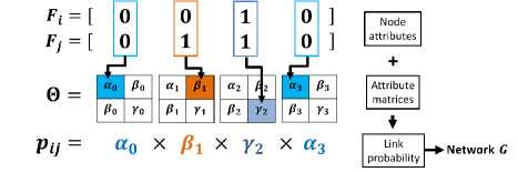
Figure 1: Multiplicative Attribute Graph (MAG) model. Each node $i$ has categorical attribute vector $F_{i}$. The probability $p_{ij}$ of edge $(i,j)$ is then determined by attributes “selecting” appropriate the entries of attribute affinity matrices $\Theta_{l}$.

Kim & Leskovec [5] proved that the MAG model captures connectivity patterns observed in real-world networks, such as heavy-tailed (power-law or log-normal) degree distributions, small diameters, unique giant connected component and local clustering of the edges. They provided both analytical and empirical evidence demonstrating that the MAG model effectively captures the structure of real-world networks.

The MAG model can handle attributes of any cardinality, however, for simplicity we limit our discussion to binary attributes. Thus, every $F_{il}$ takes value of either $0$ or $1$, and every $\Theta_{l}$ is a $2\times 2$ matrix.

Model parameter estimation. So far we have seen how given the node attributes $F$ and the corresponding attribute affinity matrices $\Theta$ we generate a MAG network. Now we focus on the reverse problem: Given a network $A$ and the number of attributes $L$ we aim to estimate affinity matrices $\Theta$ and node attributes $F$.

In other words, we aim to represent the given real network $A$ in the form of the MAG model parameters: node attributes $F=\{F_{il};i=1,\cdots,N,~{}l=1,\cdots,L\}$ and attribute affinity matrices $\Theta=\{\Theta_{l};l=1,\cdots,L\}$. MAG yields a probabilistic adjacency matrix that independently assigns the link probability to every pair of nodes, the likelihood $P(A|F,\Theta)$ of a given graph (adjacency matrix) $A$ is the product of the edge probabilities over the edges and non-edges of the network:

$$P(A|F,\Theta)=\prod_{A_{ij}=1}p_{ij}\prod_{A_{ij}=0}(1-p_{ij})$$ (2)

and $p_{ij}$ is defined in Eq. (1).

Now we can use the maximum likelihood estimation to find node attributes $F$ and their affinity matrices $\Theta$. Hence, ideally we would like to solve

$$\arg\max_{F,\Theta}P(A|F,\Theta)\,.$$ (3)

However, there are several challenges with this problem formulation. First, notice that Eq. (3) is a combinatorial problem of $O(LN)$ categorical variables even when the affinity matrices $\Theta$ are fixed. Finding both $F$ and $\Theta$ simultaneously is even harder. Second, even if we could solve this combinatorial problem, the model has a lot of parameters which may cause high variance.

To resolve these challenges, we consider a simple generative model for the node attributes. We assume that the $l$-th attribute of each node is drawn from an i.i.d. Bernoulli distribution parameterized by $\mu_{l}$. This means that the $l$-th attribute of every node takes value 1 with probability $\mu_{l}$, i.e., $F_{il}\sim Bernoulli\left(\mu_{l}\right)$.

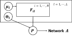
Figure 2: MAG model: Node attributes $F_{il}$ are sampled from $\mu_{l}$ and combined with affinity matrices $\Theta_{l}$ to generate a probabilistic adjacency matrix $P$.

Figure 2 illustrates the model in plate notation. First, node attributes $F_{il}$ are generated by the corresponding Bernoulli distributions $\mu_{l}$. By combining these node attributes with the affinity matrices $\Theta_{l}$, the probabilistic adjacency matrix $P$ is formed. Network $A$ is then generated by a series of coin flips where each edge $A_{ij}$ appears with probability $P_{ij}$.

Even this simplified model provably generates networks with power-law degree distributions, small diameter, and unique giant component [5]. The simplified model requires only $5L$ parameters (4 per each $\Theta_{l}$, 1 per $\mu_{l}$). Note that the number of attributes $L$ can be thought of as constant or slowly increasing in the number of nodes $N$ (e.g., $L=O(\log N)$) [2, 5].

The generative model for node attributes slightly modifies the objective function in Eq. (3). We maintain the maximum likelihood approach, but instead of directly finding attributes $F$ we now estimate parameters $\mu_{l}$ that then generate latent node attributes $F$.

We denote the log-likelihood $\log P(A|\mu,\Theta)$ as $\mathcal{L}(\mu,\Theta)$ and aim to find $\mu=\{\mu_{l}\}$ and $\Theta=\{\Theta_{l}\}$ by maximizing

$${\mathcal{L}(\mu,\Theta)=\log P(A|\mu,\Theta)=\log\sum_{F}P\left(A,F|\mu,\Theta\right)\,.}$$

Note that since $\mu$ and $\Theta$ are linked through $F$ we have to sum over all possible instantiations of node attributes $F$. Since $F$ consists of $L\cdot N$ binary variables, the number of all possible instantiations of $F$ is $O(2^{LN})$, which makes computing $\mathcal{L}(\mu,\Theta)$ directly intractable. In the next section we will show how to quickly (but approximately) compute the summation.

To compute likelihood $P\left(A,F|\mu,\Theta\right)$, we have to consider the likelihood of node attributes. Note that each edge $A_{ij}$ is independent given the attributes $F$ and each attribute $F_{il}$ is independent given the parameters $\mu_{l}$. By this conditional independence and the fact that both $A_{ij}$ and $F_{il}$ follow Bernoulli distributions with parameters $p_{ij}$ and $\mu_{l}$ we obtain

$$P(A,F|\mu,\Theta)=P(A|F,\mu,\Theta)P(F|\mu,\Theta)$$

$$=P(A|F,\Theta)P(F|\mu)$$

$$=\prod_{A_{ij}=1}p_{ij}\prod_{A_{ij}=0}(1-p_{ij})\prod_{F_{il}=0}\mu_{l}\prod_{F_{il}=1}(1-\mu_{l})$$ (4)

where $p_{ij}$ is defined in Eq. (1).

3 MAG Parameter Estimation

Now, given a network $A$, we aim to estimate the parameters $\mu_{l}$ of the node attribute model as well as the attribute affinity matrices $\Theta_{l}$. We regard the actual node attribute values $F$ as latent variables and use the expectation maximization framework.

We present the approximate method to solve the problem by developing a variational Expectation-Maximization (EM) algorithm. We first derive the lower bound $\mathcal{L}_{Q}(\mu,\Theta)$ on the true log-likelihood $\mathcal{L}(\mu,\Theta)$ by introducing the variational distribution $Q(F)$ parameterized by variational parameters $\phi$. Then, we indirectly maximize $\mathcal{L}(\mu,\Theta)$ by maximizing its lower bound $\mathcal{L}_{Q}(\mu,\Theta)$. In the E-step, we estimate $Q(F)$ by maximizing $\mathcal{L}_{Q}(\mu,\Theta)$ over the variational parameters $\phi$. In the M-step, we maximize the lower bound $\mathcal{L}_{Q}(\mu,\Theta)$ over the MAG model parameters ($\mu$ and $\Theta$) to approximately maximize the actual log-likelihood $\mathcal{L}(\mu,\Theta)$. We alternate between E- and M-steps until the parameters converge.

Variational EM. Next we introduce the distribution $Q(F)$ parameterized by variational parameters $\phi$. The idea is to define an easy-to-compute $Q(F)$ that allows us to compute the lower-bound $\mathcal{L}_{Q}(\mu,\Theta)$ of the true log-likelihood $\mathcal{L}(\mu,\Theta)$. Then instead of maximizing the hard-to-compute $\mathcal{L}$, we maximize $\mathcal{L}_{Q}$.

We now show that in order to make the gap between the lower-bound $\mathcal{L}_{Q}$ and the original log likelihood $\mathcal{L}$ small we should find the easy-to-compute $Q(F)$ that closely approximates $P(F|A,\mu,\Theta)$. For now we keep $Q(F)$ abstract and precisely define it later.

We begin by computing the lower bound $\mathcal{L}_{Q}$ in terms of $Q(F)$. We plug $Q(F)$ into $\mathcal{L}(\mu,\Theta)$ as follows:

$$\mathcal{L}(\mu,\Theta) =\log\sum_{F}P(A,F|\mu,\Theta)$$

$$=\log\sum_{F}Q(F)\frac{P(A,F|\mu,\Theta)}{Q(F)}$$

$$=\log\mathbf{E}_{Q}\left[{\frac{P(A,F|\mu,\Theta)}{Q(F)}}\right]\,.$$ (5)

As $\log x$ is a concave function, by Jensen’s inequality,

$$\log\mathbf{E}_{Q}\left[{\frac{P(A,F|\mu,\Theta)}{Q(F)}}\right]\geq\mathbf{E}_{Q}\left[{\log\frac{P(A,F|\mu,\Theta)}{Q(F)}}\right]\,.$$

Therefore, by taking

$$\mathcal{L}_{Q}(\mu,\Theta)=\mathbf{E}_{Q}\left[{\log P(A,F|\mu,\Theta)-\log Q(F)}\right]\,,$$ (6)

$\mathcal{L}_{Q}(\mu,\Theta)$ becomes the lower bound on $\mathcal{L}(\mu,\Theta)$.

Now the question is how to set $Q(F)$ so that we make the gap between $\mathcal{L}_{Q}$ and $\mathcal{L}$ as small as possible. The lower bound $\mathcal{L}_{Q}$ is tight when the proposal distribution $Q(F)$ becomes close to the true posterior distribution $P(F|A,\mu,\Theta)$ in the KL divergence. More precisely, since $P(A|\mu,\Theta)$ is independent of $F$, $\mathcal{L}(\mu,\Theta)=\log P(A|\mu,\Theta)=\mathbf{E}_{Q}\left[{\log P(A|\mu,\Theta)}\right]$. Thus, the gap between $\mathcal{L}$ and $\mathcal{L}_{Q}$ is

$$\mathcal{L}(\mu,\Theta)-\mathcal{L}_{Q}(\mu,\Theta)$$

$$=\log P(A|\mu,\Theta)-\mathbf{E}_{Q}\left[{\log P(A,F|\mu,\Theta)-\log Q(F)}\right]$$

$$=\mathbf{E}_{Q}\left[{\log P(A|\mu,\Theta)-\log P(A,F|\mu,\Theta)+\log Q(F)}\right]$$

$$=\mathbf{E}_{Q}\left[{\log P(F|A,\mu,\Theta)-\log Q(F)}\right]\,,$$

which means that the gap between $\mathcal{L}$ and $\mathcal{L}_{Q}$ is exactly the KL divergence between the proposal distribution $Q(F)$ and the true posterior distribution $P(F|A,\mu,\Theta)$.

Now we know how to choose $Q(F)$ to make the gap small. We want $Q(F)$ that is easy-to-compute and at the same time closely approximates $P(F|A,\mu,\Theta)$. We propose the following $Q(F)$ parameterized by $\phi$:

$$F_{il} \sim Bernoulli(\phi_{il})$$

$$Q_{il}(F_{il}) ={\phi_{il}}^{{F_{il}}}\left(1-{\phi_{il}}\right)^{1-{F_{il}}}$$

$$Q(F) =\prod_{i,l}Q_{il}(F_{il})$$ (7)

where $\phi=\{\phi_{il}\}$ are variational parameters and $F=\{F_{il}\}$. Our $Q(F)$ has several advantages. First, the computation of $\mathcal{L}_{Q}$ for fixed model parameters $\mu$ and $\Theta$ is tractable because $\log P(A,F|\mu,\Theta)-\log Q(F)$ in Eq. (6) is separable in terms of $F_{il}$. This means that we are able to update each $\phi_{il}$ in turn to maximize $\mathcal{L}_{Q}$ by fixing all the other parameters: $\mu$, $\Theta$ and all $\phi$ except the given $\phi_{il}$. Furthermore, since each $\phi_{il}$ represents the approximate posterior distribution of $F_{il}$ given the network, we can estimate each attribute $F_{il}$ by $\phi_{il}$.

Regularization by mutual information. In order to improve the robustness of MAG parameter estimation procedure, we enforce that each attribute is independent of others. The maximum likelihood estimation cannot guarantee the independence between the node attributes and so the solution might converge to local optima where the attributes are correlated. To prevent this, we add a penalty term that aims to minimize the mutual information (i.e., maximize the entropy) between pairs of attributes.

Since the distribution for each attribute $F_{il}$ is defined by $\phi_{il}$, we define the mutual information between a pair of attributes in terms of $\phi$. We denote this mutual information as $\mbox{MI}(F)=\sum_{l\neq l^{\prime}}\mbox{MI}_{ll^{\prime}}$ where $\mbox{MI}_{ll^{\prime}}$ represents the mutual information between the attributes $l$ and $l^{\prime}$. We then regularize the log-likelihood with the mutual information term. We arrive to the following MagFit optimization problem that we actually solve

$$\arg\max_{\phi,\mu,\Theta}\mathcal{L}_{Q}(\mu,\Theta)-\lambda\sum_{l\neq l^{\prime}}\mbox{MI}_{ll^{\prime}}\,.$$ (8)

We can quickly compute the mutual information $\mbox{MI}_{ll^{\prime}}$ between attributes $l$ and $l^{\prime}$. Let $F_{\{\cdot l\}}$ denote a random variable representing the value of attribute $l$. Then, the probability $P(F_{\{\cdot l\}}=x)$ that attribute $l$ takes value $x$ is computed by averaging $Q_{il}(x)$ over $i$. Similarly, the joint probability $P(F_{\{\cdot l\}}=x,F_{\{\cdot l^{\prime}\}}=y)$ of attributes $l$ and $l^{\prime}$ taking values $x$ and $y$ can be computed given $Q(F)$. We compute $\mbox{MI}_{ll^{\prime}}$ using $Q_{il}$ defined in Eq. (7) as follows:

$$p_{l}(x):=P(F_{\{\cdot l\}}=x)=\frac{1}{N}\sum_{i}Q_{il}(x)$$

$$p_{ll^{\prime}}(x,y):=P(F_{\{\cdot l\}}=x,F_{\{\cdot l^{\prime}\}}=y)=\frac{1}{N}\sum_{i}Q_{il}(x)Q_{il^{\prime}}(y)$$

$$\mbox{MI}_{ll^{\prime}}=\sum_{x,y\in\{0,1\}}p_{ll^{\prime}}(x,y)\log\left(\frac{p_{ll^{\prime}}(x,y)}{p_{l}(x)p_{l^{\prime}}(y)}\right)\,.$$ (9)

The MagFit algorithm. To solve the regularized MagFit problem in Eq. (8), we use the EM algorithm which maximizes the lower bound $\mathcal{L}_{Q}(\mu,\Theta)$ regularized by the mutual information. In the E-step, we reduce the gap between the original likelihood $\mathcal{L}(\mu,\Theta)$ and its lower bound $\mathcal{L}_{Q}(\mu,\Theta)$ as well as minimize the mutual information between pairs of attributes. By fixing the model parameters $\mu$ and $\Theta$, we update $\phi_{il}$ one by one using a gradient-based method. In the M-step, we then maximize $\mathcal{L}_{Q}(\mu,\Theta)$ by updating the model parameters $\mu$ and $\Theta$. We repeat E- and M-steps until all the parameters $\phi$, $\mu$, and $\Theta$ converge. Next we briefly overview the E- and the M-step. We give further details in Appendix.

Variational E-Step. In the E-step, we consider model parameters $\mu$ and $\Theta$ as given and we aim to find the values of variational parameters $\phi$ that maximize $\mathcal{L}_{Q}(\mu,\Theta)$ as well as minimize the mutual information $\mbox{MI}(F)$. We use the stochastic gradient method to update variational parameters $\phi$. We randomly select a batch of entries in $\phi$ and update them by their gradient values of the objective function in Eq. (8). We repeat this procedure until parameters $\phi$ converge.

First, by computing $\frac{\partial\mathcal{L}_{Q}}{\partial{\phi_{il}}}$ and $\frac{\partial\mbox{MI}}{\partial\phi_{il}}$, we obtain the gradient $\nabla_{\phi}\left(\mathcal{L}_{Q}(\mu,\Theta)-\lambda\mbox{MI}(F)\right)$ (see Appendix for details). Then we choose a batch of $\phi_{il}$ at random and update them by $\frac{\partial\mathcal{L}_{Q}}{\partial{\phi_{il}}}-\lambda\frac{\partial\mbox{MI}}{\partial{\phi_{il}}}$ in each step. The mutual information regularization term typically works in the opposite direction of the likelihood. Intuitively, the regularization prevents the solution from being stuck in the local optimum where the node attributes are correlated. Algorithm 1 gives the pseudocode.

Algorithm 1 MagFit-VarEStep($A,\mu,\Theta$)

  Initialize $\phi^{(0)}=\{\phi_{il}:i=1,\cdots,N,\quad l=1,\cdots,L\}$

    

  for $t\leftarrow 0$ to $T-1$ do

     $\phi^{(t+1)}\leftarrow\phi^{(t)}$

     Select $S\subset\phi^{(t)}$ with $|S|=B$

     for $\phi_{il}^{(t)}\in S$ do

        Compute $\frac{\partial\mathcal{L}_{Q}}{\partial{\phi_{il}}}$

        $\frac{\partial\mbox{MI}}{\partial{\phi_{il}}}\leftarrow 0$

        for $l^{\prime}\neq l$ do

           Compute $\frac{\partial\mbox{MI}_{ll^{\prime}}}{\partial\phi_{il}}$

           $\frac{\partial\mbox{MI}}{\partial{\phi_{il}}}\leftarrow\frac{\partial\mbox{MI}}{\partial{\phi_{il}}}+\frac{\partial\mbox{MI}_{ll^{\prime}}}{\partial\phi_{il}}$

        end for

        $\phi_{il}^{(t+1)}\leftarrow\phi_{il}^{(t)}+\eta(\frac{\partial\mathcal{L}_{Q}}{\partial{\phi_{il}}}-\lambda\frac{\partial\mbox{MI}}{\partial{\phi_{il}}})$

     end for

  end for

Algorithm 2 MagFit-VarMStep($\phi$, $G$, $\Theta^{(0)}$)

    

  for $l\leftarrow 1$ to $L$ do

     $\mu_{l}\leftarrow\frac{1}{N}\sum_{i}\phi_{il}$

  end for

    

  for $t\leftarrow 0$ to $T-1$ do

     for $l\leftarrow 1$ to $L$ do

        $\Theta^{(t+1)}_{l}\leftarrow\Theta^{(t)}_{l}+\eta\nabla_{\Theta_{l}}\mathcal{L}_{Q}$

     end for

  end for

Variational M-Step. In the E-step, we introduced the variational distribution $Q(F)$ parameterized by $\phi$ and approximated the posterior distribution $P(F|A,\mu,\Theta)$ by maximizing $\mathcal{L}_{Q}(\mu,\Theta)$ over $\phi$. In the M-step, we now fix $Q(F)$, i.e., fix the variational parameters $\phi$, and update the model parameters $\mu$ and $\Theta$ to maximize $\mathcal{L}_{Q}$.

First, in order to maximize $\mathcal{L}_{Q}(\mu,\Theta)$ with respect to $\mu$, we need to maximize $\mathcal{L}_{\mu_{l}}=\sum_{i}\mathbf{E}_{Q_{il}}\left[{\log P(F_{il}|\mu_{l})}\right]$ for each $\mu_{l}$. By definitions in Eq. (4) and (7), we obtain

$$\mathcal{L}_{\mu_{l}}=\sum_{i}\left(\phi_{il}\mu_{il}+(1-\phi_{il})(1-\mu_{il})\right)\,.$$

Then $\mathcal{L}_{\mu_{l}}$ is maximized when

$$\frac{\partial\mathcal{L}_{\mu_{l}}}{\partial\mu_{l}}=\sum_{i}\phi_{il}-N=0$$

where $\mu_{l}=\frac{1}{N}\sum_{i}\phi_{il}$.

Second, to maximize $\mathcal{L}_{Q}(\mu,\Theta)$ with respect to $\Theta_{l}$, we maximize $\mathcal{L}_{\Theta}=\mathbf{E}_{Q}\left[{\log P(A,F|\mu,\Theta)-\log Q(F)}\right]$. We first obtain the gradient

$$\nabla_{\Theta_{l}}\mathcal{L}_{\Theta}=\sum_{i,j}\nabla_{\Theta_{l}}\mathbf{E}_{Q_{i,j}}\left[{\log P(A_{ij}|F_{i},F_{j},\Theta)}\right]$$ (10)

and then use a gradient-based method to optimize $\mathcal{L}_{Q}(\mu,\Theta)$ with regard to $\Theta_{l}$. Algorithm 2 gives details for optimizing $\mathcal{L}_{Q}(\mu,\Theta)$ over $\mu$ and $\Theta$.

Speeding up MagFit. So far we described how to apply the variational EM algorithm to MAG model parameter estimation. However, both E-step and M-step are infeasible when the number of nodes $N$ is large. In particular, in the E-step, for each update of $\phi_{il}$, we have to compute the expected log-likelihood value of every entry in the $i$-th row and column of the adjacency matrix $A$. It takes $O(LN)$ time to do this, so overall $O(L^{2}N^{2})$ time is needed to update all $\phi_{il}$. Similarly, in the M-step, we need to sum up the gradient of $\Theta_{l}$ over every pair of nodes (as in Eq. (10)). Therefore, the M-step requires $O(LN^{2})$ time and so it takes $O(L^{2}N^{2})$ to run a single iteration of EM. Quadratic dependency in the number of attributes $L$ and the number of nodes $N$ is infeasible for the size of the networks that we aim to work with here.

To tackle this, we make the following observation. Note that both Eq. (10) and computation of $\frac{\partial\mathcal{L}_{Q}}{\partial{\phi_{il}}}$ involve the sum of expected values of the log-likelihood or the gradient. If we can quickly approximate this sum of the expectations, we can dramatically reduce the computation time. As real-world networks are sparse in a sense that most of the edges do not exist in the network, we can break the summation into two parts — a fixed part that “pretends” that the network has no edges and the adjustment part that takes into account the edges that actually exist in the network.

For example, in the M-step we can separate Eq. (10) into two parts, the first term that considers an empty graph and the second term that accounts for the edges that actually occurred in the network:

$$\nabla_{\Theta_{l}}\mathcal{L}_{\Theta}=\sum_{i,j}\nabla_{\Theta_{l}}\mathbf{E}_{Q_{i,j}}\left[{\log P(0|F_{i},F_{j},\Theta)}\right]$$

$$\quad+\sum_{A_{ij}=1}\nabla_{\Theta_{l}}\mathbf{E}_{Q_{i,j}}\left[{\log P(1|F_{i},F_{j},\Theta)-\log P(0|F_{i},F_{j},\Theta)}\right]\,.$$ (11)

Now we approximate the first term that computes the gradient pretending that the graph $A$ has no edges:

$$\sum_{i,j}\nabla_{\Theta_{l}}\mathbf{E}_{Q_{i,j}}\left[{\log P(0|F_{i},F_{j},\Theta)}\right]$$

$$=\nabla_{\Theta_{l}}\mathbb{E}_{Q_{i,j}}[\sum_{i,j}\log P(0|F_{i},F_{j},\Theta)]$$

$$\approx\nabla_{\Theta_{l}}\mathbf{E}_{Q_{i,j}}\left[{N(N-1)\mathbb{E}_{F}[\log P(0|F,\Theta)]}\right]$$

$$=\nabla_{\Theta_{l}}N(N-1)\mathbb{E}_{F}[\log P(0|F,\Theta)]\,.$$ (12)

Since each $F_{il}$ follows the Bernoulli distribution with parameter $\mu_{l}$, Eq. (12) can be computed in $O(L)$ time. As the second term in Eq. (11) requires only $O(LE)$ time, the computation time of the M-step is reduced from $O(LN^{2})$ to $O(LE)$. Similarly we reduce the computation time of the E-step from $O(L^{2}N^{2})$ to $O(L^{2}E)$ (see Appendix for details). Thus overall we reduce the computation time of MagFit from $O(L^{2}N^{2})$ to $O(L^{2}E)$.

4 Experiments

Having introduced the MAG model estimation procedure MagFit, we now turn our attention to evaluating the fitting procedure itself and the ability of the MAG model to capture the connectivity structure of real networks. There are three goals of our experiments: (1) evaluate the success of MagFit parameter estimation procedure; (2) given a network, infer both latent node attributes and the affinity matrices to accurately model the network structure; (3) given a network where nodes already have attributes, infer the affinity matrices. For each experiment, we proceed by describing the experimental setup and datasets.

Convergence of MagFit. First, we briefly evaluate the convergence of the MagFit algorithm. For this experiment, we use synthetic MAG networks with $N=1024$ and $L=4$. Figure 3(a) illustrates that the objective function $\mathcal{L}_{Q}$, i.e., the lower bound of the log-likelihood, nicely converges with the number of EM iterations. While the log-likelihood converges, the model parameters $\mu$ and $\Theta$ also nicely converge. Figure 3(b) shows convergence of $\mu_{1},\dots,\mu_{4}$, while Fig. 3(c) shows the convergence of entries $\Theta_{l}[0,0]$ for $l=1,\dots,4$. Generally, in 100 iterations of EM, we obtain stable parameter estimates.

We also compare the runtime of the fast MagFit to the naive version where we do not use speedups for the algorithm. Figure 3(d) shows the runtime as a function of the number of nodes in the network. The runtime of the naive algorithm scales quadratically $O(N^{2})$, while the fast version runs in near-linear time. For example, on 4,000 node network, the fast algorithm runs about 100 times faster than the naive one.

(a) Convergence of $\mathcal{L}_{Q}(\mu,\Theta)$

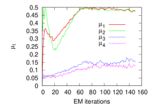
(b) Convergence of $\mu_{l}$’s

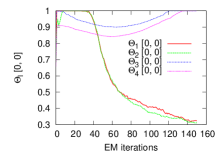
(c) Convergence of $\Theta_{l}{[0,0]}$’s

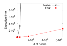
(d) Run time

Figure 3: Parameter convergence and scalability.

Based on these experiments, we conclude that the variational EM gives robust parameter estimates. We note that the MagFit optimization problem is non-convex, however, in practice we observe fast convergence and good fits. Depending on the initialization MagFit may converge to different solutions but in practice solutions tend to have comparable log-likelihoods and consistently good fits. Also, the method nicely scales to networks with up to hundred thousand nodes.

Experiments on real data. We proceed with experiments on real datasets. We use the LinkedIn social network [8] at the time in its evolution when it had $N=$ 4,096 nodes and $E=$ 10,052 edges. We also use the Yahoo!-Answers question answering social network, again from the time when the network had $N=$ 4,096, $E=$ 5,678 [8]. For our experiments we choose $L=11$, which is roughly $\log N$ as it has been shown that this is the optimal choice for $L$ [5].

Now we proceed as follows. Given a real network $A$, we apply MagFit to estimate MAG model parameters $\hat{\Theta}$ and $\hat{\mu}$. Then, given these parameters, we generate a synthetic network $\hat{A}$ and compare how well synthetic $\hat{A}$ mimics the real network $A$.

Evaluation. To measure the level of agreement between synthetic $\hat{A}$ and the real $A$, we use several different metrics. First, we evaluate how well $\hat{A}$ captures the structural properties, like degree distribution and clustering coefficient, of the real network $A$. We consider the following network properties:

• In/Out-degree distribution (InD/OutD) is a histogram of the number of in-coming and out-going links of a node.

• Singular values (SVal) indicate the singular values of the adjacency matrix versus their rank.

• Singular vector (SVec) represents the distribution of components in the left singular vector associated with the largest singular value.

• Clustering coefficient (CCF) represents the degree versus the average (local) clustering coefficient of nodes of a given degree [18].

• Triad participation (TP) indicates the number of triangles that a node is adjacent to. It measures the transitivity in networks.

Since distributions of the above quantities are generally heavy-tailed, we plot them in terms of complementary cumulative distribution functions ($P(X>x)$ as a function of $x$). Also, to indicate the scale, we do not normalize the distributions to sum to 1.

Second, to quantify the discrepancy of network properties between real and synthetic networks, we use a variant of Kolmogorov-Sminorv (KS) statistic and the $L2$ distance between different distributions. The original KS statistics is not appropriate here since if the distribution follows a power-law then the original KS statistics is usually dominated by the head of the distribution. We thus consider the following variant of the KS statistic: $\textit{KS}(D_{1},D_{2})=\max_{x}|\log D_{1}(x)-\log D_{2}(x)|$ [6], where $D_{1}$ and $D_{2}$ are two complementary cumulative distribution functions. Similarly, we also define a variant of the $L2$ distance on the log-log scale, $\textit{L2}(D_{1},D_{2})=\sqrt{\frac{1}{\log b-\log a}\left(\int_{a}^{b}\left(\log D_{1}(x)-\log D_{2}(x)\right)^{2}\,d(\log x)\right)}$ where $[a,b]$ is the support of distributions ${D_{1}}$ and ${D_{2}}$. Therefore, we evaluate the performance with regard to the recovery of the network properties in terms of the KS and L2 statistics.

Last, since MAG generates a probabilistic adjacency matrix $P$, we also evaluate how well $P$ represents a given network $A$. We use the following two metrics:

• Log-likelihood (LL) measures the possibility that the probabilistic adjacency matrix $P$ generates network $A$: $LL=\sum_{ij}\log(P_{ij}^{A_{ij}}(1-P_{ij})^{1-A_{ij}})$.

• True Positive Rate Improvement (TPI) represents the improvement of the true positive rate over a random graph: $TPI=\sum_{A_{ij}=1}P_{ij}/\frac{E^{2}}{N^{2}}$. TPI indicates how much more probability mass is put on the edges compared to a random graph (where each edge occurs with probability $E/N^{2}$).

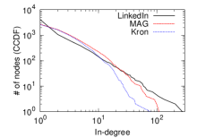
(a) In-degree

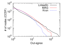
(b) Out-degree

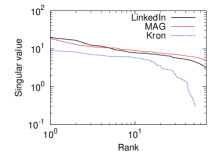
(c) Singular value

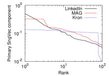
(d) Singular vector

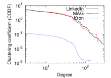
(e) Clustering coefficient

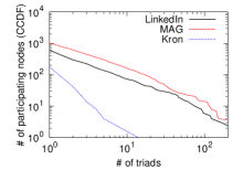
(f) Triad participation

Figure 4: The recovered network properties by the MAG model and the Kronecker graphs model on the LinkedIn network. For every network property, MAG model outperforms the Kronecker graphs model.

Table 1: KS and L2 of MAG and the Kronecker graphs model on the LinkedIn network. MAG exhibits 50-70% better performance than Kronecker graphs model.

KS	InD	OutD	SVal	SVec	TP	CCF	Avg
MAG	3.70	3.80	0.84	2.43	3.87	3.16	2.97
Kron	4.00	4.32	1.15	7.22	8.08	6.90	5.28
L2
MAG	1.01	1.15	0.46	0.62	1.68	1.11	1.00
Kron	1.54	1.57	0.65	6.14	6.00	4.33	3.37

Recovery of the network structure. We begin our investigations of real networks by comparing the performance of the MAG model to that of the Kronecker graphs model [9], which offers a state of the art baseline for modeling the structure of large networks. We use evaluation methods described in the previous section where we fit both models to a given real-world network $A$ and generate synthetic $\hat{A}_{MAG}$ and $\hat{A}_{Kron}$. Then we compute the structural properties of all three networks and plot them in Figure 4. Moreover, for each of the properties we also compute KS and L2 statistics and show them in Table 1.

Figure 4 plots the six network properties described above for the LinkedIn network and the synthetic networks generated by fitting MAG and Kronecker models to the LinkedIn network. We observe that MAG can successfully produce synthetic networks that match the properties of the real network. In particular, both MAG and Kronecker graphs models capture the degree distribution of the LinkedIn network well. However, MAG model performs much better in matching spectral properties of graph adjacency matrix as well as the local clustering of the edges in the network.

Table 1 shows the KS and L2 statistics for each of the six structural properties plotted in Figure 4. Results confirm our previous visual inspection. The MAG model is able to fit the network structure much better than the Kronecker graphs model. In terms of the average KS statistics, we observe 43% improvement, while observe even greater improvement of 70% in the L2 metric. For degree distributions and the singular values, MAG outperforms Kronecker for about 25% while the improvement on singular vector, triad participation and clustering coefficient is 60 $\sim$ 75%.

We make similar observations on the Yahoo!-Answers network but omit the results for brevity. We include them in Appendix.

(a) Homophily	(b) Heterophily	(c) Core-Periphery

Figure 5: Structures in which a node attribute can affect link affinity. The widths of arrows correspond to the affinities towards link formation.

We interpret the improvement of the MAG over Kronecker graphs model in the following way. Intuitively, we can think of Kronecker graphs model as a version of the MAG model where all affinity matrices $\Theta_{l}$ are the same and all $\mu_{l}=0.5$. However, real-world networks may include various types of structures and thus different attributes may interact in different ways. For example, Figure 5 shows three possible linking affinities of a binary attribute. Figure 5(a) shows a homophily (love of the same) attribute affinity and the corresponding affinity matrix $\Theta$. Notice large values on the diagonal entries of $\Theta$, which means that link probability is high when nodes share the same attribute value. The top of each figure demonstrates that there will be many links between nodes that have the value of the attribute set to “0” and many links between nodes that have the value “1”, but there will be few links between nodes where one has value “0” and the other “1”. Similarly, Figure 5(b) shows a heterophily (love of the different) affinity, where nodes that do not share the value of the attribute are more likely to link, which gives rise to near-bipartite networks. Last, Figure 5(c) shows a core-periphery affinity, where links are most likely to form between “0” nodes (i.e., members of the core) and least likely to form between “1” nodes (i.e., members of the periphery). Notice that links between the core and the periphery are more likely than the links between the nodes of the periphery.

Turning our attention back to MAG and Kronecker models, we note that real-world networks globally exhibit nested core-periphery structure [9] (Figure 5(c)). While there exists the core (densely connected) and the periphery (sparsely connected) part of the network, there is another level of core-periphery structure inside the core itself. On the other hand, if viewing the network more finely, we may also observe the homophily which produces local community structure. MAG can model both global core-periphery structure and local homophily communities, while the Kronecker graphs model cannot express the different affinity types because it uses only one initiator matrix.

For example, the LinkedIn network consists of 4 core-periphery affinities, 6 homophily affinities, and 1 heterophily affinity matrix. Core-periphery affinity models active users who are more likely to connect to others. Homophily affinities model people who are more likely to connect to others in the same job area. Interestingly, there is a heterophily affinity which results in bipartite relationship. We believe that the relationships between job seekers and recruiters or between employers and employees leads to this structure.

Table 2: LL and TPI values for LinkedIn (LI) and Yahoo!-Answers (YA) networks

	LL(LI)	TPI (LI)	LL(YA)	TPI (YA)
MAG	-47663	232.8	-33795	192.2
Kron	-87520	10.0	-48204	5.4

TPI and LL. We also compare the LL and TPI values of MAG and Kronecker models on both LinkedIn and Yahoo!-Answers networks. Table 2 shows that MAG outperforms Kronecker graphs by surprisingly large margin. In LL metric, the MAG model shows $50\sim\,60$ % improvement over the Kronecker model. Furthermore, in TPI metric, the MAG model shows $23\sim\,35$ times better accuracy than the Kronecker model. From these results, we conclude that the MAG model achieves a superior probabilistic representation of a given network.

Case Study: AddHealth network. So far we considered node attributes as latent and we inferred the affinity matrices $\Theta$ as well as the attributes themselves. Now, we consider the setting where the node attributes are already given and we only need to infer affinities $\Theta$. Our goal here is to study how real attributes explain the underlying network structure.

We use the largest high-school friendship network ($N=$ 457, $E=$ 2,259) from the National Longitudinal Study of Adolescent Health (AddHealth) dataset. The dataset includes more than 70 school-related attributes for each student. Since some attributes do not take binary values, we binarize them by taking value 1 if the value of the attribute is less than the median value. Now we aim to investigate which attributes affect the friendship formation and how.

We set $L=7$ and consider the following methods for selecting a subset of 7 attributes:

• R7: Randomly choose 7 real attributes and fit the model (i.e., only fit $\Theta$ as attributes are given).

• L7: Regard all 7 attributes as latent (i.e., not given) and estimate $\mu_{l}$ and $\Theta_{l}$ for $l=1,\dots,7$.

• F7: Forward selection. Select attributes one by one. At each step select an additional attribute that maximizes the overall log-likelihood (i.e., select a real attribute and estimate its $\Theta_{l}$).

• F5+L2: Select 5 real attributes using forward selection. Then, we infer 2 more latent attributes.

To make the MagFit work with fixed real attributes (i.e., only infer $\Theta$) we fix $\phi_{il}$ to the values of real attributes. In the E-step we then optimize only over the latent set of $\phi_{il}$ and the M-step remains as is.

AddHealth network structure. We begin by evaluating the recovery of the network structure. Figure 6 shows the recovery of six network properties for each attribute selection method. We note that each method manages to recover degree distributions as well as spectral properties (singular values and singular vectors) but the performance is different for clustering coefficient and triad participation.

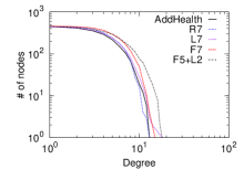
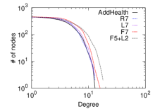
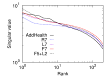
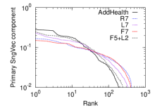
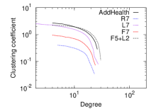
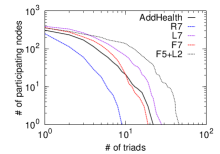
Figure 6: Properties of the AddHealth network.

Table 3: Performance of different selection methods.

KS	InD	OutD	SVal	SVec	TP	CCF	Avg
R7	1.00	0.58	0.48	2.92	4.52	4.45	2.32
F7	2.32	2.80	0.30	2.68	2.60	1.58	2.05
F5+L2	3.45	4.00	0.26	0.95	1.30	3.45	2.24
L7	1.58	1.58	0.18	2.00	2.67	2.66	1.78
L2
R7	0.25	0.16	0.25	0.96	3.18	1.74	1.09
F7	0.71	0.67	0.18	0.98	1.26	0.78	0.76
F5+L2	0.80	0.87	0.13	0.34	0.76	1.30	0.70
L7	0.29	0.27	0.10	0.64	0.75	1.22	0.54

Table 3 shows the discrepancies in the 6 network properties (KS and L2 statistics) for each attribute selection method. As expected, selecting 7 real attributes at random (R7) performs the worst. Naturally, L7 performs the best (23% improvement over R7 in KS and 50% in L2) as it has the most degrees of freedom. It is followed by F5+L2 (the combination of 5 real and 2 latent attributes) and F7 (forward selection).

As a point of comparison we also experimented with a simple logistic regression classifier where given the attributes of a pair of nodes we aim to predict an occurrence of an edge. Basically, given network $A$ on $N$ nodes, we have $N^{2}$ (one for each pair of nodes) training examples: $E$ are positive (edges) and $N^{2}-E$ are negative (non-edges). However, the model performs poorly as it gives 50% worse KS statistics than MAG. The average KS of logistic regression under R7 is 3.24 (vs. 2.32 of MAG) and the same statistic under F7 is 3.00 (vs. 2.05 of MAG). Similarly, logistic regression gives 40% worse L2 under R7 and 50% worse L2 under F7. These results demonstrate that using the same attributes MAG heavily outperforms logistic regression. We understand that this performance difference arises because the connectivity between a pair of nodes depends on some factors other than the linear combination of their attribute values.

Table 4: LL and TPI for the AddHealth network.

	R7	F7	F5+L2	L7
LL	-13651	-12161	-12047	-9154
TPI	1.0	1.1	1.9	10.0

Last, we also examine the LL and TPI values and compare them to the random attribute selection R7 as a baseline. Table 4 gives the results. Somewhat contrary to our previous observations, we note that F7 only slightly outperforms R7, while F5+L2 gives a factor 2 better TPI than R7. Again, L7 gives a factor 10 improvement in TPI and overall best performance.

Table 5: Affinity matrices of 5 AddHealth attributes.

Affinity matrix	Attribute description
[0.572 0.146; 0.146 0.999]	School year (0 if $\geq$ 2)
[0.845 0.332; 0.332 0.816]	Highest level math (0 if $\geq$ 6)
[0.788 0.377; 0.377 0.784]	Cumulative GPA (0 if $\geq$ 2.65)
[0.999 0.246; 0.246 0.352]	AP/IB English (0 if taken)
[0.794 0.407; 0.407 0.717]	Foreign language (0 if taken)

Attribute affinities. Last, we investigate the structure of attribute affinity matrices to illustrate how MAG model can be used to understand the way real attributes interact in shaping the network structure. We use forward selection (F7) to select 7 real attributes and estimate their affinity matrices. Table 5 reports first 5 attributes selected by the forward selection.

First notice that AddHealth network is undirected graph and that the estimated affinity matrices are all symmetric. This means that without a priori biasing the fitting towards undirected graphs, the recovered parameters obey this structure. Second, we also observe that every attribute forms a homophily structure in a sense that each student is more likely to be friends with other students of the same characteristic. For example, people are more likely to make friends of the same school year. Interestingly, students who are freshmen or sophomore are more likely (0.99) to form links among themselves than juniors and seniors (0.57). Also notice that the level of advanced courses that each student takes as well as the GPA affect the formation of friendship ties. Since it is difficult for students to interact if they do not take the same courses, the chance of the friendships may be low. We note that, for example, students that take advanced placement (AP) English courses are very likely to form links. However, links between students who did not take AP English are nearly as likely as links between AP and non-AP students. Last, we also observe relatively small effect of the number of foreign language courses taken on the friendship formation.

5 Conclusion

We developed MagFit, a scalable variational expectation maximization method for parameter estimation of the Multiplicative Attribute Graph model. The model naturally captures interactions between node attributes and the network structure. MAG model considers nodes with categorical attributes and the probability of an edge between a pair of nodes depends on the product of individual attribute link formation affinities. Experiments show that MAG reliably captures the network connectivity patterns as well as provides insights into how different attributes shape the structure of networks. Venues for future work include settings where node attributes are partially missing and investigations of other ways to combine individual attribute linking affinities into a link probability.

Acknowledgements

Research was in-part supported by NSF CNS-1010921, NSF IIS-1016909, AFRL FA8650-10-C-7058, LLNL DE-AC52-07NA27344, Albert Yu & Mary Bechmann Foundation, IBM, Lightspeed, Yahoo and the Microsoft Faculty Fellowship.

Appendix A Variational EM Algorithm

In Section 2, we proposed a version of MAG model by introducing a generative Bernoulli model for node attributes and formulated the problem to solve. In the following Section 3, we gave a sketch of MagFit that used the variational EM algorithm to solve the problem. Here we provide how to compute the gradients of the model parameters ($\phi$, $\mu$, and $\Theta$) for the of E-step and M-step that we omitted in Section 3. We also give the details of the fast MagFit in the following.

A.1 Variational E-Step

In the E-step, the MAG model parameters $\mu$ and $\Theta$ are given and we aim to find the optimal variational parameter $\phi$ that maximizes $\mathcal{L}_{Q}(\mu,\Theta)$ as well as minimizes the mutual information factor $\mbox{MI}(F)$. We randomly select a batch of entries in $\phi$ and update the selected entries by their gradient values of the objective function $\mathcal{L}_{Q}(\mu,\Theta)$. We repeat this updating procedure until $\phi$ converges.

In order to obtain $\nabla_{\phi}\left(\mathcal{L}_{Q}(\mu,\Theta)-\lambda\mbox{MI}(F)\right)$, we compute $\frac{\partial\mathcal{L}_{Q}}{\partial{\phi_{il}}}$ and $\frac{\partial\mbox{MI}}{\partial\phi_{il}}$ in turn as follows.

Computation of $\frac{\partial\mathcal{L}_{Q}}{\partial{\phi_{il}}}$. To calculate the partial derivative $\frac{\partial\mathcal{L}_{Q}}{\partial{\phi_{il}}}$, we begin by restating $\mathcal{L}_{Q}(\mu,\Theta)$ as a function of one specific parameter $\phi_{il}$ and differentiate this function over $\phi_{il}$. For convenience, we denote $F_{-il}=\{F_{jk}:j\neq i,k\neq l\}$ and $Q_{-il}=\prod_{j\neq i,k\neq l}Q_{jk}$. Note that $\sum_{F_{il}}Q_{il}(F_{il})=1$ and $\sum_{F_{-il}}Q_{-il}(F_{-il})$ because both are the sums of probabilities of all possible events. Therefore, we can separate $\mathcal{L}_{Q}(\mu,\Theta)$ in Eq. (6) into the terms of $Q_{il}(F_{il})$ and $Q_{-il}(F_{-il})$:

$$\mathcal{L}_{Q}(\mu,\Theta)$$

$$=\mathbf{E}_{Q}\left[{\log P(A,F|\mu,\Theta)-\log Q(F)}\right]$$

$$=\sum_{F}Q\left(F\right)\left(\log P\left(A,F|\mu,\Theta\right)-\log Q\left(F\right)\right)$$

$$=\sum_{F_{-il}}\sum_{F_{il}}Q_{-il}(F_{-il})Q_{il}(F_{il})$$

$$\quad\times\left(\log P\left(A,F|\mu,\Theta\right)-\log Q_{il}\left(F_{il}\right)-\log Q_{-il}\left(F_{-il}\right)\right)$$

$$=\sum_{F_{il}}Q_{il}(F_{il})\left(\sum_{F_{-il}}Q_{-il}\left(F_{-il}\right)\log P\left(A,F|\mu,\Theta\right)\right)$$

$$\quad\quad-\sum_{F_{il}}Q_{il}(F_{il})\log Q_{il}(F_{il})$$

$$\quad\quad-\sum_{F_{-il}}Q_{-il}(F_{-il})\log Q_{-il}(F_{-il})$$

$$=\sum_{F_{il}}Q_{il}(F_{il})\mathbf{E}_{Q_{-il}}\left[{\log P\left(A,F|\mu,\Theta\right)}\right]$$

$$\quad\quad+\mathcal{H}(Q_{il})+\mathcal{H}(Q_{-il})$$ (13)

where $\mathcal{H}(P)$ represents the entropy of distribution $P$.

Since we compute the gradient of $\phi_{il}$, we regard the other variational parameter $\phi_{-il}$ as a constant so $\mathcal{H}(Q_{-il})$ is also a constant. Moreover, as $\mathbf{E}_{Q_{-il}}\left[{\log P\left(A,F|\mu,\Theta\right)}\right]$ integrates out all the terms with regard to $\phi_{-il}$, it is a function of $F_{il}$. Thus, for convenience, we denote $\mathbf{E}_{Q_{-il}}\left[{\log P\left(A,F|\mu,\Theta\right)}\right]$ as $\log\tilde{P_{il}}\left({F_{il}}\right)$. Then, since $F_{il}$ follows a Bernoulli distribution with parameter $\phi_{il}$, by Eq. (13)

$$\mathcal{L}_{Q}(\mu,\theta) =(1-\phi_{il})\left(\log\tilde{P_{il}}\left({1}\right)-\log(1-\phi_{il})\right)$$

$$\quad+\phi_{il}\left(\log\tilde{P_{il}}\left({0}\right)-\log\phi_{il}\right)+const\,.$$ (14)

Note that both $\tilde{P_{il}}\left({0}\right)$ and $\tilde{P_{il}}\left({1}\right)$ are constant. Therefore,

$$\frac{\partial\mathcal{L}_{Q}}{\partial{\phi_{il}}}=\log\frac{\tilde{P_{il}}\left({0}\right)}{\phi_{il}}-\log\frac{\tilde{P_{il}}\left({1}\right)}{1-\phi_{il}}\,.$$ (15)

To complete the computation of $\frac{\partial\mathcal{L}_{Q}}{\partial{\phi_{il}}}$, now we focus on the value of $\tilde{P_{il}}\left({F_{il}}\right)$ for $F_{il}=0,1$. By Eq. (4) and the linearity of expectation, $\log\tilde{P_{il}}\left({F_{il}}\right)$ is separable into small tractable terms as follows:

$$\log\tilde{P_{il}}\left({F_{il}}\right) =\mathbf{E}_{Q_{-il}}\left[{\log P(A,F|\mu,\Theta)}\right]$$

$$=\sum_{u,v}\mathbf{E}_{Q_{-il}}\left[{\log P(A_{uv}|F_{u},F_{v},\Theta)}\right]$$

$$\quad+\sum_{u,k}\mathbf{E}_{Q_{-il}}\left[{\log P(F_{uk}|\mu_{k})}\right]$$ (16)

where $F_{i}=\{F_{il}:l=1,2,\cdots,L\}$. However, if $u,v\neq i$, then $\mathbf{E}_{Q_{-il}}\left[{\log P(A_{uv}|F_{u},F_{v},\Theta)}\right]$ is a constant, because the average over $Q_{-il}(F_{-il})$ integrates out all the variables $F_{u}$ and $F_{v}$. Similarly, if $u\neq i$ and $k\neq l$, then $\mathbf{E}_{Q_{-il}}\left[{\log P(F_{uk}|\mu_{k})}\right]$ is a constant. Since most of terms in Eq. (16) are irrelevant to $\phi_{il}$, $\log\tilde{P_{il}}\left({F_{il}}\right)$ is simplified as

$$\log\tilde{P_{il}}\left({F_{il}}\right) =\left(\sum_{j}\mathbf{E}_{Q_{-il}}\left[{\log P(A_{ij}|F_{i},F_{j},\Theta)}\right]\right)$$

$$\quad+\left(\sum_{j}\mathbf{E}_{Q_{-il}}\left[{\log P(A_{ji}|F_{j},F_{i},\Theta)}\right]\right)$$

$$\quad+\log P(F_{il}|\mu_{l})+C$$ (17)

for some constant $C$.

By definition of $P(F_{il}|\mu_{l})$ in Eq. (4), the last term in Eq. (17) is

$$\log P(F_{il}|\mu_{l})=F_{il}\log\mu_{l}+(1-F_{il})\log(1-\mu_{il})\,.$$ (18)

With regard to the first two terms in Eq. (17),

$$\log P(A_{ij}|F_{i},F_{j},\Theta)=\log P(A_{ji}|F_{i},F_{j},\Theta^{T})\,.$$

Hence, the methods to compute the two terms are equivalent. Thus, we now focus on the computation of $\mathbf{E}_{Q_{-il}}\left[{\log P(A_{ij}|F_{i},F_{j},\Theta)}\right]$.

First, in case of $A_{ij}=1$, by definition of $P(A_{ij}|F_{i},F_{j})$ in Eq. (4),

$$\mathbf{E}_{Q_{-il}}\left[{\log P(A_{ij}=1|F_{i},F_{j},\Theta)}\right]$$

$$=\mathbf{E}_{Q_{-il}}\left[{\sum_{k}\log\Theta_{k}[F_{ik},F_{jk}]}\right]$$

$$=\mathbf{E}_{Q_{jl}}\left[{\log\Theta_{l}[F_{il},F_{jl}]}\right]+\sum_{k\neq l}\mathbf{E}_{Q_{ik,jk}}\left[{\log\Theta_{k}[F_{ik},F_{jk}]}\right]$$

$$=\mathbf{E}_{Q_{jl}}\left[{\log\Theta_{l}[F_{il},F_{jl}]}\right]+C^{\prime}$$ (19)

for some constant $C^{\prime}$ where $Q_{ik,jk}(F_{ik},F_{jk})=Q_{ik}(F_{ik})Q_{jk}(F_{jk})$, because $\mathbf{E}_{Q_{ik,jk}}\left[{\log\Theta_{k}[F_{ik},F_{jk}]}\right]$ is constant for each $k$.

Second, in case of $A_{ij}=0$,

$$P(A_{ij}=0|F_{i},F_{j},\Theta) =1-\prod_{k}\Theta_{k}[F_{ik},F_{jk}]\,.$$ (20)

Since $\log P(A_{ij}|F_{i},F_{j},\Theta)$ is not separable in terms of $\Theta_{k}$, it takes $O(2^{2L})$ time to compute $\mathbf{E}_{Q_{-il}}\left[{\log P(A_{ij}|F_{i},F_{j},\Theta)}\right]$ exactly. We can reduce this computation time to $O(L)$ by applying Taylor’s expansion of $\log(1-x)\approx-x-\frac{1}{2}x^{2}$ for small $x$:

$$\mathbf{E}_{Q_{-il}}\left[{\log P(A_{ij}=0|F_{i},F_{j},\Theta)}\right]$$

$$\approx\mathbf{E}_{Q_{-il}}\left[{-\prod_{k}\Theta_{k}[F_{ik},F_{jk}]-\frac{1}{2}\prod_{k}\Theta^{2}_{k}[F_{ik},F_{jk}]}\right]$$

$$=-\mathbf{E}_{Q_{jl}}\left[{\Theta_{l}[F_{il},F_{jl}]}\right]\prod_{k\neq l}\mathbf{E}_{Q_{ik,jk}}\left[{\Theta_{k}[F_{ik},F_{jk}]}\right]$$

$$\quad\quad-\frac{1}{2}\mathbf{E}_{Q_{jl}}\left[{\Theta^{2}_{l}[F_{il},F_{jl}]}\right]\prod_{k\neq l}\mathbf{E}_{Q_{ik,jk}}\left[{\Theta^{2}_{k}[F_{ik},F_{jk}]}\right]$$ (21)

where each term can be computed by

$$\mathbf{E}_{Q_{il}}\left[{Y_{l}[F_{il},F_{jl}]}\right] =\phi_{jl}Y_{l}[F_{il},0]+(1-\phi_{jl})Y_{l}[F_{il},1]$$

$$\mathbf{E}_{Q_{ik,jk}}\left[{Y_{k}[F_{ik},F_{jk}]}\right] =[\phi_{ik}~{}~{}\phi_{jk}]\cdot Y_{k}\cdot[1-\phi_{ik}~{}~{}1-\phi_{jk}]^{T}$$

for any matrix $Y_{l},Y_{k}\in\mathbb{R}^{2\times 2}$.

In brief, for fixed $i$ and $l$, we first compute $\mathbf{E}_{Q_{-il}}\left[{\log P(A_{ij}|F_{i},F_{j},\Theta)}\right]$ for each node $j$ depending on whether or not $i\rightarrow j$ is an edge. By adding $\log P(F_{il}|\mu_{l})$, we then acheive the value of $\log\tilde{P_{il}}\left({F_{il}}\right)$ for each $F_{il}$. Once we have $\log\tilde{P_{il}}\left({F_{il}}\right)$, we can finally compute $\frac{\partial\mathcal{L}_{Q}}{\partial{il}}$.

Scalable computation. However, as we analyzed in Section 3, the above E-step algorithm requires $O(LN)$ time for each computation of $\frac{\partial\mathcal{L}_{Q}}{\partial{\phi_{il}}}$ so that the total computation time is $O(L^{2}N^{2})$, which is infeasible when the number of nodes $N$ is large.

Here we propose the scalable algorithm of computing $\frac{\partial\mathcal{L}_{Q}}{\partial{\phi_{il}}}$ by further approximation. As described in Section 3, we quickly approximate the value of $\frac{\partial\mathcal{L}_{Q}}{\partial{\phi_{il}}}$ as if the network would be empty, and adjust it by the part where edges actually exist. To approximate $\frac{\partial\mathcal{L}_{Q}}{\partial{\phi_{il}}}$ in empty network case, we reformulate the first term in Eq. (17):

$$\sum_{j}\mathbf{E}_{Q_{-il}}\left[{\log P(A_{ij}|F_{i},F_{j},\Theta)}\right]=\sum_{j}\mathbf{E}_{Q_{-il}}\left[{\log P(0|F_{i},F_{j},\Theta)}\right]$$

$$\quad+\sum_{A_{ij}=1}\mathbf{E}_{Q_{-il}}\left[{\log P(1|F_{i},F_{j},\Theta)-\log P(0|F_{i},F_{j},\Theta)}\right]$$ (22)

However, since the sum of i.i.d. random variables can be approximated in terms of the expectaion of the random variable, the first term in Eq. (22) can be approximated as follows:

$$\sum_{j}\mathbf{E}_{Q_{-il}}\left[{\log P(0|F_{i},F_{j},\Theta)}\right]$$

$$=\mathbf{E}_{Q_{-il}}\left[{\sum_{j}\log P(0|F_{i},F_{j},\Theta)}\right]$$

$$\approx\mathbf{E}_{Q_{-il}}\left[{(N-1)\mathbb{E}_{F_{j}}[\log P(0|F_{i},F_{j},\Theta)]}\right]$$

$$=(N-1)\mathbb{E}_{F_{j}}[\log P(0|F_{i},F_{j},\Theta)]$$ (23)

As $F_{jl}$ marginally follows a Bernoulli distribution with $\mu_{l}$, we can compute Eq. (23) by using Eq. (21) in $O(L)$ time. Since the second term of Eq. (22) takes $O(LN_{i})$ time where $N_{i}$ represents the number of neighbors of node $i$, Eq. (22) takes only $O(LN_{i})$ time in total. As in the E-step we do this operation by iterating for all $i$’s and $l$’s, the total computation time of the E-step eventually becomes $O(L^{2}E)$, which is feasible in many large-scale networks.

Computation of $\frac{\partial\mbox{MI}}{\partial{\phi_{il}}}$. Now we turn our attention to the derivative of the mutual information term. Since $\mbox{MI}(F)=\sum_{l\neq l^{\prime}}\mbox{MI}_{ll^{\prime}}$, we can separately compute the derivative of each term $\frac{\partial\mbox{MI}_{ll^{\prime}}}{\partial\phi_{il}}$. By definition in Eq. (9) and Chain Rule,

$$\frac{\partial\mbox{MI}_{ll^{\prime}}}{\partial\phi_{il}}=\sum_{x,y\in\{0,1\}}\frac{\partial p_{ll^{\prime}}(x,y)}{\partial\phi_{il}}\log\frac{p_{ll^{\prime}}(x,y)}{p_{l}(x)p_{l^{\prime}}(y)}$$

$$\quad+\frac{\partial p_{ll^{\prime}}(x,y)}{\partial\phi_{il}}+\frac{p_{ll^{\prime}}(x,y)}{p_{l}(x)}\frac{\partial p_{l}(x)}{\partial\phi_{il}}+\frac{p_{ll^{\prime}}(x,y)}{p_{l^{\prime}}(y)}\frac{\partial p_{l^{\prime}}(y)}{\partial\phi_{il}}\,.$$ (24)

The values of $p_{ll^{\prime}}(x,y)$, $p_{l}(x)$, and $p_{l^{\prime}}(y)$ are defined in Eq. (9). Therefore, in order to compute $\frac{\partial\mbox{MI}_{ll^{\prime}}}{\partial\phi_{il}}$, we need the values of $\frac{\partial p_{ll^{\prime}}(x,y)}{\partial\phi_{il}}$, $\frac{\partial p_{l}(x)}{\partial\phi_{il}}$, and $\frac{\partial p_{l^{\prime}}(y)}{\partial\phi_{il}}$. By definition in Eq. (9),

$$\frac{\partial p_{ll^{\prime}}(x,y)}{\partial\phi_{il}}=Q_{il^{\prime}}(y)\frac{\partial Q_{il}}{\partial\phi_{il}}$$

$$\frac{\partial p_{l}(x)}{\partial\phi_{il}}=\frac{\partial Q_{il}}{\partial\phi_{il}}$$

$$\frac{\partial p_{l^{\prime}}(y)}{\partial\phi_{il}}=0$$

where $\frac{\partial Q_{il}}{\partial\phi_{il}}|_{F_{il}=0}=1$ and $\frac{\partial Q_{il}}{\partial\phi_{il}}|_{F_{il}=1}=-1$.

Since all terms in $\frac{\partial\mbox{MI}_{ll^{\prime}}}{\partial\phi_{il}}$ are tractable, we can eventually compute $\frac{\partial\mbox{MI}}{\partial{\phi_{il}}}$.

A.2 Variational M-Step

In the E-Step, with given model parameters $\mu$ and $\Theta$, we updated the variational parameter $\phi$ to maximize $\mathcal{L}_{Q}(\mu,\Theta)$ as well as to minimize the mutual information between every pair of attributes. In the M-step, we basically fix the approximate posterior distribution $Q(F)$, i.e. fix the variational parameter $\phi$, and update the model parameters $\mu$ and $\Theta$ to maximize $\mathcal{L}_{Q}(\mu,\Theta)$.

To reformulate $\mathcal{L}_{Q}(\mu,\Theta)$ by Eq. (4),

$$\mathcal{L}_{Q}(\mu,\Theta)$$

$$=\mathbf{E}_{Q}\left[{\log P(A,F|\mu,\Theta)-\log Q(F)}\right]$$

$$=\mathbf{E}_{Q}\left[{\sum_{i,j}P(A_{ij}|F_{i},F_{j},\Theta)+\sum_{i,l}P(F_{il}|\mu_{l})}\right]+\mathcal{H}(Q)$$

$$=\sum_{i,j}\mathbf{E}_{Q_{i,j}}\left[{\log P(A_{ij}|F_{i},F_{j},\Theta)}\right]$$

$$\quad+\sum_{l}\left(\sum_{i}\mathbf{E}_{Q_{il}}\left[{\log P(F_{il}|\mu_{l})}\right]\right)+\mathcal{H}(Q)$$ (25)

where $Q_{i,j}(F_{\{i\cdot\}},F_{\{j\cdot\}})$ represents $\prod_{l}Q_{il}(F_{il})Q_{jl}(F_{jl})$.

After all, $\mathcal{L}_{Q}(\mu,\Theta)$ in Eq. (25) is divided into the following terms: a function of $\Theta$, a function of $\mu_{l}$, and a constant. Thus, we can exclusively update $\mu$ and $\Theta$. Since we already showed how to update $\mu$ in Section 3, here we focus on the maximization of $\mathcal{L}_{\Theta}=\mathbf{E}_{Q}\left[{\log P(A,F|\mu,\Theta)-\log Q(F)}\right]$ using the gradient method.

Computation of $\nabla_{\Theta_{l}}\mathcal{L}_{\Theta}$. To use the gradient method, we need to compute the gradient of $\mathcal{L}_{\Theta}$:

$$\nabla_{\Theta_{l}}\mathcal{L}_{\Theta}=\sum_{i,j}\nabla_{\Theta_{l}}\mathbf{E}_{Q_{i,j}}\left[{\log P(A_{ij}|F_{i},F_{j},\Theta)}\right]\,.$$ (26)

We separately calculate the gradient of each term in $\mathcal{L}_{\Theta}$ as follows: For every $z_{1},z_{2}\in\{0,1\}$, if $A_{ij}=1$,

$$\frac{\partial\mathbf{E}_{Q_{i,j}}\left[{\log P(A_{ij}|F_{i},F_{j},\Theta)}\right]}{\partial\Theta_{l}[z_{1},z_{2}]}\bigg{|}_{A_{ij}=1}$$

$$=\frac{\partial}{\partial\Theta_{l}[z_{1},z_{2}]}\mathbf{E}_{Q_{i,j}}\left[{\sum_{k}\log\Theta_{k}[F_{ik},F_{jk}]}\right]$$

$$=\frac{\partial}{\partial\Theta_{l}[z_{1},z_{2}]}\mathbf{E}_{Q_{i,j}}\left[{\log\Theta_{l}[F_{il},F_{jl}]}\right]$$

$$=\frac{Q_{il}(z_{1})Q_{jl}(z_{2})}{\Theta_{l}[z_{1},z_{2}]}\,.$$ (27)

On the contrary, if $A_{ij}=0$, we use Taylor’s expansion as used in Eq. (21):

$$\frac{\partial\mathbf{E}_{Q_{i,j}}\left[{\log P(A_{ij}|F_{i},F_{j},\Theta)}\right]}{\partial\Theta_{l}[z_{1},z_{2}]}\bigg{|}_{A_{ij}=0}$$

$$\approx\frac{\partial}{\partial\Theta_{l}}\mathbf{E}_{Q_{i,j}}\left[{-\prod_{k}\Theta_{k}[F_{ik},F_{jk}]-\frac{1}{2}\prod_{k}\Theta^{2}_{k}[F_{ik},F_{jk}]}\right]$$

$$=-Q_{il}(z_{1})Q_{jl}(z_{2})\prod_{k\neq l}\mathbf{E}_{Q_{ik,jk}}\left[{\Theta_{k}[F_{ik},F_{jk}]}\right]$$

$$\quad\quad-Q_{il}(z_{1})Q_{jl}(z_{2})\Theta_{k}[z_{1},z_{2}]\prod_{k\neq l}\mathbf{E}_{Q_{ik,jk}}\left[{\Theta^{2}_{k}[F_{ik},F_{jk}]}\right]$$ (28)

where $Q_{il,jl}(F_{il},F_{jl})=Q_{il}(F_{il})Q_{jl}(F_{jl})$.

Since

$$\mathbf{E}_{Q_{ik,jk}}\left[{f(\Theta)}\right]=\sum_{z_{1},z_{2}}Q_{ik}(z_{1})Q_{jk}(z_{2})f\left(\Theta[z_{1},z_{2}]\right)$$

for any function $f$ and we know each function values of $Q_{il}(F_{il})$ in terms of $\phi_{il}$, we are able to achieve the gradient $\nabla_{\Theta_{l}}\mathcal{L}_{\Theta}$ by Eq. (26) $\sim$ (28).

Scalable computation. The M-step requires to sum $O(N^{2})$ terms in Eq. (26) where each term takes $O(L)$ time to compute. Similarly to the E-step, here we propose the scalable algorithm by separating Eq. (26) into two parts, the fixed part for an empty graph and the adjustment part for the actual edges:

$$\nabla_{\Theta_{l}}\mathcal{L}_{\Theta}=\sum_{i,j}\nabla_{\Theta_{l}}\mathbf{E}_{Q_{i,j}}\left[{\log P(0|F_{i},F_{j},\Theta)}\right]$$

$$\quad+\sum_{A_{ij}=1}\nabla_{\Theta_{l}}\mathbf{E}_{Q_{i,j}}\left[{\log P(1|F_{i},F_{j},\Theta)-\log P(0|F_{i},F_{j},\Theta)}\right]\,.$$ (29)

We are able to approximate the first term in Eq. (29), the value for the empty graph part, as follows:

$$\sum_{i,j}\nabla_{\Theta_{l}}\mathbf{E}_{Q_{i,j}}\left[{\log P(0|F_{i},F_{j},\Theta)}\right]$$

$$=\nabla_{\Theta_{l}}\mathbf{E}_{Q_{i,j}}\left[{\sum_{i,j}\log P(0|F_{i},F_{j},\Theta)}\right]$$

$$\approx\nabla_{\Theta_{l}}\mathbf{E}_{Q_{i,j}}\left[{N(N-1)\mathbb{E}_{F}[\log P(0|F,\Theta)]}\right]$$

$$=\nabla_{\Theta_{l}}N(N-1)\mathbb{E}_{F}[\log P(0|F,\Theta)]\,.$$ (30)

Since each $F_{il}$ marginally follows the Bernoulli distribution with $\mu_{l}$, Eq. (30) is computed by Eq. (28) in $O(L)$ time. As the second term in Eq. (29) requires only $O(LE)$ time, the computation time of the M-step is finally reduced to $O(LE)$ time.

Appendix B Experiments

B.1 Yahoo!-Ansers Network

Here we add some experimental results that we omitted in Section 4. First, Figure 7 compares the six network properties of Yahoo!-Answers network and the synthetic networks generated by MAG model and Kronecker graphs model fitted to the real network. The MAG model in general shows better performance than the Kronecker graphs model. Particularly, the MAG model greatly outperforms the Kronecker graphs model in local-clustering properties (clustering coefficient and triad participation).

Second, to quantify the recovery of the network properties, we show the KS and L2 statistics for the synthetic networks generated by MAG model and Kronecker graphs model in Table 6. Through Table 6, we can confirm the visual inspection in Figure 7. The MAG model shows better statistics than the Kronecker graphs model in overall and there is huge improvement in the local-clustering properties.

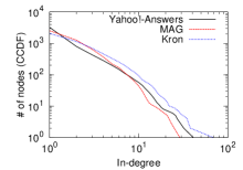
(a) In-degree

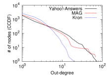
(b) Out-degree

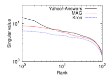
(c) Singular value

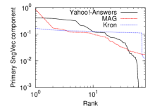
(d) Singular vector

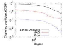
(e) Clustering coefficient

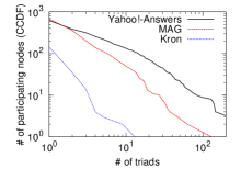
(f) Triad participation

Figure 7: The recovered network properties by the MAG model and the Kronecker graphs model on the Yahoo!-Answers network. For every network property, MAG model outperforms the Kronecker graphs model.

Table 6: KS and L2 for MAG and Kronecker model fitted to Yahoo!-Answers network

KS	InD	OutD	SVal	SVec	TP	CCF	Avg
MAG	3.00	2.80	14.93	13.72	4.84	4.80	7.35
Kron	2.00	5.78	13.56	15.47	7.98	7.05	8.64
L2
MAG	0.96	0.74	0.70	6.81	2.76	2.39	2.39
Kron	0.81	2.24	0.69	7.41	6.14	4.73	3.67

B.2 AddHealth Network

We briefly mentioned the logistic regression method in AddHealth network experiment. Here we provide the details of the logistic regression and full experimental results of it.

For the variables of the logistic regression, we use a set of real attributes in the AddHealth network dataset. For such set of attributes, we used F7 (forward selection) and R7 (random selection) defined in Section 4. Once the set of attributes is fixed, we come up with a linear model:

$$P(i\rightarrow j)=\frac{\exp(c+\sum_{l}\alpha_{l}F_{il}+\sum_{l}\beta_{l}F_{jl})}{1+\exp(c+\sum_{l}\alpha_{l}F_{il}+\sum_{l}\beta_{l}F_{jl})}\,.$$

Table 7 shows the KS and L2 statistics for logistic regression methods under R7 and F7 attribute sets. It seems that the logistic regression succeeds in the recovery of degree distributions. However, it fails to recover the local-clustering properties (clustering coefficient and triad participation) for both sets.

Table 7: KS and L2 for logistic regression methods fitted to AddHealth network

KS	InD	OutD	SVal	SVec	TP	CCF	Avg
R7	2.00	2.58	0.58	3.03	5.39	5.91	3.24
F7	1.59	1.59	0.52	3.03	5.43	5.91	3.00
L2
R7	0.54	0.58	0.29	1.09	3.43	2.42	1.39
F7	0.42	0.24	0.27	1.12	3.55	2.09	1.28

References

- [1] E. M. Airoldi, D. M. Blei, S. E. Fienberg, and E. P. Xing. Mixed membership stochastic blockmodels. JMLR, 9:1981–2014, 2007.
- [2] A. Bonato, J. Janssen, and P. Pralat. The geometric protean model for on-line social networks. In WAW ’10, 2010.
- [3] M. Faloutsos, P. Faloutsos, and C. Faloutsos. On power-law relationships of the internet topology. In SIGCOMM ’99, pages 251–262, 1999.
- [4] P. Hoff, A. Raftery, and M. Handcock. Latent space approaches to social network analysis. Journal of the American Statistical Association, 97:1090–1098, 2002.
- [5] M. Kim and J. Leskovec. Multiplicative attribute graph model of real-world networks. In WAW ’10, 2010.
- [6] M. Kim and J. Leskovec. Network completion problem: Inferring missing nodes and edges in networks. In SDM ’11, 2011.
- [7] R. Kumar, P. Raghavan, S. Rajagopalan, D. Sivakumar, A. Tomkins, and E. Upfal. Stochastic models for the web graph. In FOCS ’00, page 57, 2000.
- [8] J. Leskovec, L. Backstrom, R. Kumar, and A. Tomkins. Microscopic evolution of social networks. In KDD ’08, pages 462–470, 2008.
- [9] J. Leskovec, D. Chakrabarti, J. Kleinberg, C. Faloutsos, and Z. Ghahramani. Kronecker Graphs: An Approach to Modeling Networks. JMLR, 2010.
- [10] J. Leskovec, D. Chakrabarti, J. M. Kleinberg, and C. Faloutsos. Realistic, mathematically tractable graph generation and evolution, using kronecker multiplication. In PKDD ’05, pages 133–145, 2005.
- [11] J. Leskovec and C. Faloutsos. Scalable modeling of real graphs using kronecker multiplication. In ICML ’07, 2007.
- [12] J. Leskovec, J. M. Kleinberg, and C. Faloutsos. Graphs over time: densification laws, shrinking diameters and possible explanations. In KDD ’05, 2005.
- [13] M. Mahdian and Y. Xu. Stochastic kronecker graphs. In WAW ’07, pages 179–186, 2007.
- [14] L. Page, S. Brin, R. Motwani, and T. Winograd. The pagerank citation ranking: Bringing order to the web. Technical report, Stanford Dig. Lib. Tech. Proj., 1998.
- [15] G. Palla, L. Lovasz, and T. Vicsek. Multifractal network generator. PNAS, 107(17):7640–7645, 2010.
- [16] G. Robins and P. Pattison and Y. Kalish and D. Lusher An introduction to exponential random graph (p*) models for social networks. Social Networks, 29(2):173–191, 2007.
- [17] P. Sarkar and A. W. Moore. Dynamic social network analysis using latent space models. SIGKDD Explorations, 7:31–40, December 2005.
- [18] D. J. Watts and S. H. Strogatz. Collective dynamics of ’small-world’ networks. Nature, 393:440–442, 1998.
- [19] S. J. Young and E. R. Scheinerman. Random Dot Product Graph Models for Social Networks, volume 4863 of Lecture Notes in Computer Science. 2007.