Thermodynamic, Dynamic, Structural and Excess Entropy Anomalies for core-softened potentials

Abstract

Using molecular dynamic simulations we study three families of continuous core-softened potentials consisting of two length scales: a shoulder scale and an attractive scale. All the families have the same slope between the two length scales but exhibit different potential energy gap between them. For each family three shoulder depths are analyzed. We show that all these systems exhibit a liquid-liquid phase transition between a high density liquid phase and a low density liquid phase ending at a critical point. The critical temperature is the same for all cases suggesting that the critical temperature is only dependent on the slope between the two scales. The critical pressure decreases with the decrease of the potential energy gap between the two scales suggesting that the pressure is responsible for forming the high density liquid. We also show, using the radial distribution function and the excess entropy analysis, that the density, the diffusion and the structural anomalies are present if particles move from the attractive scale to the shoulder scale with the increase of the temperature indicating that the anomalous behavior depends only in what happens up to the second coordination shell.

I Introduction

The phase behavior of single component systems as particles interacting via the so-called core-softened $(CS)$ potentials is receiving a lot of attention recently. These potentials exhibit a repulsive core with a softening region with a shoulder or a ramp [1, 2, 3, 4, 5, 6, 7, 8]. These models originates from the desire of constructing a simple two-body isotropic potential capable of describing the complicated features of systems interacting via anisotropic potentials. This procedure generates systems that are analytically and computationally tractable and that one hopes are capable to retain the qualitative features of the real complex systems [9, 10, 11, 12].

The physical motivation behind these studies is the recently acknowledged possibility that some single component systems interacting through a core-softened potential display density and diffusion anomalies. This opened the discussion about the relation between the existence of thermodynamic anomalies in liquids and the form of the effective potential [13, 14, 15, 16, 17, 18].

These anomalies appear in two different ways. First, it is the density anomaly. Most liquids contract upon cooling. This is not the case of water and other fluid systems. For water the specific volume at ambient pressure starts to increase when cooled below $T\approx 4^{o}C$. The anomalous behavior of water was first suggested 300 years ago [19] and was confirmed by a number of experiments [9, 10]. Besides, between $0.1$ MPa and $190$ MPa water also exhibits an anomalous increase of compressibility [20, 21] and, at atmospheric pressure, an increase of isobaric heat capacity upon cooling [22, 23].

Experiments for Te, [24] Ga, Bi, [25] S, [26, 27] and Ge₁₅Te₈₅, [11] and simulations for silica, [12, 28, 29, 30] silicon [31] and BeF₂, [12] show the same density anomaly.

But density anomaly is not the only unusual behavior that these materials have. For a normal liquid the diffusion constant, $D$, decreases under compression. This is not the case of water. $D$ increases on compression at low temperature, $T$, up to a maximum $D_{\rm max}(T)$ at $p=p_{D\mathrm{max}}(T)$. [10, 32]. Numerical simulations for SPC/E water [33] recover the experimental results and show that the anomalous behavior of $D$ extends to the metastable liquid phase of water at negative pressure, a region that is difficult to access for experiments [34, 35, 36, 37]. In this region the diffusivity $D$ decreases for decreasing $p$ until it reaches a minimum value $D_{\rm min}(T)$ at some pressure $p_{D\mathrm{min}}(T)$, and the normal behavior, with $D$ increasing for decreasing $p$, is reestablished only for $p<p_{D\mathrm{min}}(T)$ [34, 38, 39, 35, 36, 37]. Besides water, silica [29, 28] and silicon [40] also exhibit a diffusion anomalous region.

Acknowledging that CS potentials may engender density and diffusion anomalous behavior, a number of CS potentials were proposed to model the anisotropic systems described above. They possess a repulsive core that exhibits a region of softening where the slope changes dramatically. This region can be a shoulder or a ramp [1, 41, 42, 43, 44, 45, 46, 47, 48, 49, 50, 6, 51, 52, 53, 54, 55, 56, 57, 15, 16, 58, 59]. These models exhibit density and diffusion anomalies, but depending on the specific shape of the potential, the anomalies might be hidden in the metastable phase [16]. Also there are a number of core-softened potentials in which the anomalies are not present [60, 61]. The relation between the specific shape of the effective core-softened potential and the microscopic mechanism necessary for the presence of the anomalies is still under debate [62, 57, 16, 63].

Recently it was suggested that the link between the presence of the density and diffusion anomaly and the microscopic details of the system can be analyzed in the framework of the excess-entropy-based formalism [64] applied to similar systems by Errington et al. [65] and Chakraborty and Chakravarty [66]. Within this approach the presence of the density and the diffusion anomalies are related to the density dependence of the excess entropy, $s_{\mathrm{ex}}$.

The computation of the excess entropy, however, requires integrating the radial distribution function in the whole space. The anomalous behavior, however, seems to depend only in the two length scales present in the system and, therefore, should not depend on the particle distributions far away. Here we propose that two length scales potentials will have density and diffusion anomalies if the two scales would be accessible. In principle the accessibility only depends in the distribution of particles in these two distances. Therefore, the knowledge of the complete excess entropy is not necessary for knowing if the system has or not anomalies. The behavior of the partial excess entropy, computed only up to the second coordination shell should give enough information to determine if a system has anomalies or not.

In this paper we test this assumption by computing the pressure-temperature phase diagram and the excess entropy for three families of core-softened potentials that have two length scale: a shoulder scale and an attractive scale [67, 18]. In all the three families the slope between the two scales is the same [13]. The shoulder scale is made more favorable by decreasing the energy gap between the two length scales (see potentials A, B and C in Fig. 1). In addition the shoulder scale becomes more favorable by making the depth of the shoulder scale deeper (see potentials A1, A2 and A3 in Fig. 1). The slope between the two length scales is kept fixed in order to have the liquid-liquid critical point and the density anomalous region in the same region of the pressure temperature phase diagram [13].

The remaining of this paper goes as follows. In Sec. II the model is introduced. The simulations details are given Sec. III. In Sec. IV the results are discussed. Finally, Sec. V presents the conclusion.

II The Model

We consider a system of $N$ particles, with diameter $\sigma$, where the pair interaction is described by a family of continuous potentials given by

$$\centering U(r)=\epsilon\left[\left(\frac{\sigma}{r}\right)^{a}-\left(\frac{\sigma}{r}\right)^{b}\right]+\sum_{j=1}^{4}h_{j}\exp\left[-\left(\frac{r-c_{j}}{w_{j}}\right)^{2}\right]\;\;.\@add@centering$$ (1)

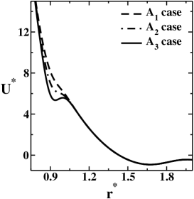
(a) Values of $c_{1}=0.90c^{ref}$, $h_{1}=0.30h^{ref},0.60h^{ref}$ and $0.90h^{ref}$.

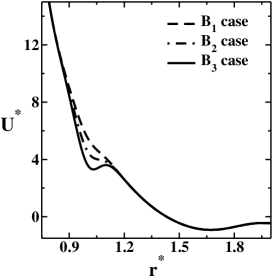
(b) Values of $c_{1}=1.00c^{ref}$, $h_{1}=0.25h^{ref},0.50h^{ref}$ and $0.75h^{ref}$.

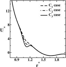
(c) Values of $c_{1}=1.10c^{ref}$, $h_{1}=0.22h^{ref},0.44h^{ref}$ and $0.66h^{ref}$.

Figure 1: Interaction potential obtained by changing parameters $h_{1}$ in the Eq. (1).The potential and the distances are in dimensionless units $U^{*}=U/\gamma$ and $r^{*}=r/r_{0}$.Here we use $\epsilon/\gamma=0.02$ and $\sigma/r_{0}=1.47$.

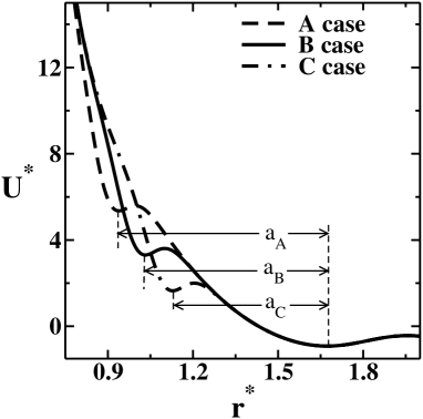
(a)  Distance between the scales.

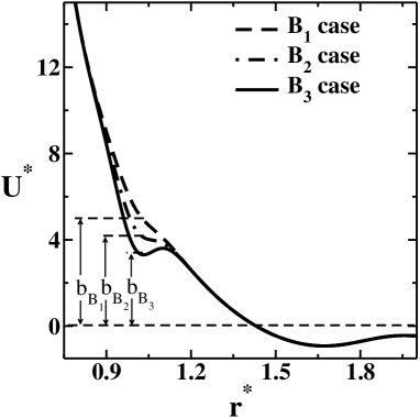
(b)  Different depths of the first scale.

Figure 2: Scheme to distinguish the distance between the scales and depths of the first scale.

The first term is a Lennard-Jones potential and the second term is composed by four Gaussians, each Gaussian is centered in $c_{j}$. This potential can represent a whole family of intermolecular interactions, depending of the choice of the parameters $a,b,\sigma,\{h_{j},c_{j},w_{j}\}$, with $j=1,\dots,4$. The values of these parameters are in Table 1. The parameters are chosen in order to obtain a two length scale potential [67, 68, 69] that is related to the interaction between two tetramers [67, 68].

The simulations are made in dimensionless units, therefore all the physical quantities are given in terms of the energy scale $\gamma$ and the distance scale $r_{0}$ where $\gamma$ is the energy scale and $r_{0}$ is the length scale chosen so the minimum of the potential in the $B_{3}$ case is about $r^{*}=1$. The distance scale is chosen so the minimum of the shoulder scale in the $B_{3}$ case Here we use $\epsilon/\gamma=0.02$ and $\sigma/r_{0}=1.47$.

Modifying the parameters $c_{1}$ and $h_{1}$ in the Eq. (1), according to Table 2, allow us to change the depth of the shoulder well, as illustrated in Fig. 1. Here we use nine different values for $h_{1}$ and they are expressed as a multiple of a reference value $h_{1}^{ref}$. We also use three different values of $c_{1}$ and they are expressed as a multiple of a reference value $c_{1}^{ref}$. For all the nine cases the values of $a,b,\{w_{j}\}$ with $j=1,\dots,4$, ${c_{i}}$ with $i=2,\dots,3$, $h^{ref}$ and $c^{href}$. Table 1 gives the parameter values in $\AA$ and $kcal/mol$ consistent with modeling ST4 water [67].

Modifying the distance between the two minima of the two scales, shoulder scale $(SC)$ and attractive scale $(AS)$, leads to the three families $A$, $B$ and $C$ as shown in Fig. 1. The changes in the distance between the two length scales were done in such way to preserve the slope between the two scales and, therefore, to have in all the cases the region of density anomaly in the same region of the pressure-temperature phase diagram as proposed by Yan et. al [70].

The family $A$ has the largest distance and the largest potential energy gap between the two length scales ($a_{A}=0.72$ in Fig. 2), the family $B$ has the intermediate distance and intermediate potential energy gap between the two length scales ($a_{B}=0.62$ in Fig. 2), and the family $C$ has the shortest distance and the smallest potential energy gap between the two length scales, ($a_{C}=0.52$ in Fig. 2).

For each family, we analyze three different depths of the shoulder scale represented by $1$, $2$ and $3$ (see Fig. 2). The potentials $1$ have the most shallow shoulder scale , the potentials $2$ have intermediate shoulder depth and the potentials $3$ have the deepest shoulder scale. Table 3 gives the values for the depths for each one of the families.

In summary, we analyze nine different potentials: $A_{1},A_{2},A_{3},B_{1},B_{2},B_{3},C_{1},C_{2}$ and $C_{3}$ as illustrated in Fig. 1. The values of the different $h_{1}$ for each case are listed in Table 2.

Barraz et al. [18] investigated the family $B$. It was shown that this potential exhibits thermodynamic, dynamic and structural anomalies if the shoulder scale is not too deep. Their result suggests that in order to have anomalies it is necessary but no sufficient to have two length scales competing. Both length scales must be accessible. When the shoulder scale becomes too deep the particles are trapped in this length scale and no anomaly is present. By making the shoulder deeper we are decreasing the difference in energy between the scales and therefore destroying the competition.

Here we explore the accessibility or the absence of accessibility by changing both the energy gap between the two length scales and the distance between them.

III The Simulation Details

The properties of the system were obtained by $NVT$ molecular dynamics using Nose-Hoover heat-bath with coupling parameter $Q=2$. The system is characterized by 500 particles in a cubic box with periodic boundary conditions, interacting with the intermolecular potential described above. All physical quantities are expressed in reduced units [71] given by

$$t^{*} = tr_{0}(m/\gamma)^{1/2}$$

$$T^{*} = \frac{k_{B}T}{\gamma}$$

$$p^{*} = \frac{pr_{0}^{3}}{\gamma}$$

$$\rho^{*} = \rho r_{0}^{3}$$

$$D^{*} = D\sqrt{\frac{m}{\gamma r_{0}^{2}}}\;\;.$$ (2)

Standard periodic boundary conditions together with predictor-corrector algorithm were used to integrate the equations of motion with a time step $\Delta t^{*}=0.002$ and potential cut off radius $r_{c}^{*}=3.5$. The initial configuration were set on solid and on liquid states and, in both cases, the equilibrium state was reached after $t_{eq}^{*}=1000$ (what is in fact $500,000$ steps since $\Delta t^{*}=0.002$). From this time on the physical quantities were stored in intervals of $\Delta t_{R}^{*}=1$ during $t_{R}^{*}=1000$. The system is uncorrelated after $t_{d}^{*}=10$, from the velocity auto-correlation function. With $50$ descorrelated samples were used to get the average of the physical quantities.

The thermodynamic stability of the system was checked by analyzing the dependence of pressure on density namely

$$\frac{\partial p}{\partial\rho}<0$$ (3)

, by the behavior of the energy and also by visual analysis of the final structure, searching for cavitation.

At the phase boundary between the liquid and the amorphous phases we found stable states points at both phases. The state with the lower energy was considered. In this particular region of the pressure-temperature phase diagram the energy was a good approximation for the Helmoltz free energy.

The error bars for temperatures and pressures away from the critical region are smaller than the size of the gray lines. The error bar near the critical point are $\Delta T=0.0025$ and $\Delta p=0.05$. Our error is controlled by making averages of uncorrelated measures.

Table 1: Parameters for potentials A, B and C in reduced unit.

Parameter	Value	Parameter	Value	Parameter	Value	Parameter	Value
$a$	$9.056$	$w_{1}$	$0.085$	$c_{1}^{ref}$	$0.996$	$h_{1}^{ref}$	$-3.79$
$b$	$4.044$	$w_{2}$	$0.618$	$c_{2}$	$0.529$	$h_{2}$	$1.209$
$\epsilon$	$0.020$	$w_{3}$	$0.826$	$c_{3}$	$1.598$	$h_{3}$	$-1.503$
$\sigma$	$1.475$	$w_{4}$	$0.214$	$c_{4}$	$1.929$	$h_{4}$	$0.767$

Table 2: Parameters of $c_{1}$ and $h_{1}$ for potentials A, B and C.

Potentials	Values	Potentials	Values	Potentials	Values	Potentials	Values
$A$	$0.90\,c_{1}^{ref}$	$A_{1}$	$0.30\,h_{1}^{ref}$	$B_{1}$	$0.25\,h_{1}^{ref}$	$C_{1}$	$0.22\,h_{1}^{ref}$
$B$	$1.00\,c_{1}^{ref}$	$A_{2}$	$0.60\,h_{1}^{ref}$	$B_{2}$	$0.50\,h_{1}^{ref}$	$C_{2}$	$0.44\,h_{1}^{ref}$
$C$	$1.10\,c_{1}^{ref}$	$A_{3}$	$0.90\,h_{1}^{ref}$	$B_{3}$	$0.75\,h_{1}^{ref}$	$C_{3}$	$0.66\,h_{1}^{ref}$

Table 3: Values for the depths for each one of the families.

Potential	Value	Potential	Value	Potential	Value
$b_{A_{1}}$	$7.10$	$b_{B_{1}}$	$4.94$	$b_{C_{1}}$	$2.95$
$b_{A_{2}}$	$6.20$	$b_{B_{2}}$	$4.07$	$b_{C_{2}}$	$2.33$
$b_{A_{3}}$	$5.28$	$b_{B_{3}}$	$3.32$	$b_{C_{3}}$	$1.60$

IV Results

Pressure-Temperature Phase Diagram

First, we explore the effects that the increase of the shoulder depth and the decrease of the distance between the two scales have in the location in the pressure-temperature phase diagram of the different phases. Fig. 3 illustrates the pressure versus temperature phase diagram of the three families $A$, $B$ and $C$ of potentials. At high temperatures there are a fluid phase and a gas phase (not shown). These two phases coexist at a first order line that ends at a critical point (see Table 4 for the pressure and the temperature values).

At low temperatures and high pressures there are two liquid phases coexisting at a first order line ending at a second critical point (see Table 5 for the pressure and the temperature values). The thermodynamic stability of the state points was checked by analyzing the dependence of pressure on density using Eq. 3. The critical point was identified in the graph by the region where isochores cross. The coexistence line was obtained as the medium line between the stability limit of each phase.

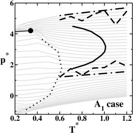
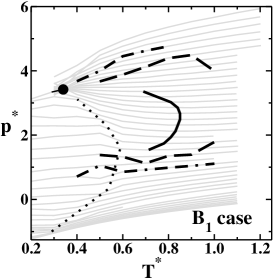
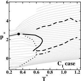
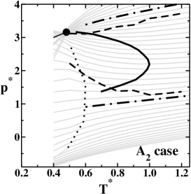
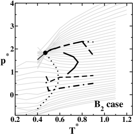
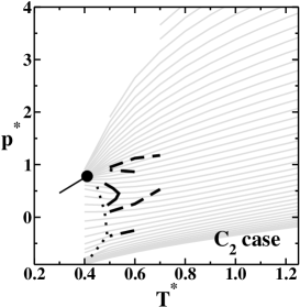
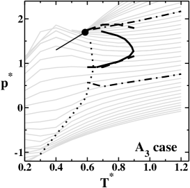
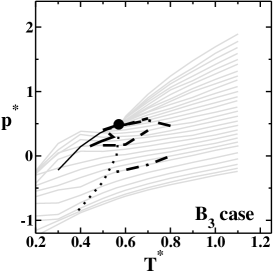
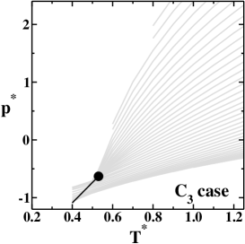
Figure 3: Pressure-temperature phase diagram for the family $A$ in the left-hand side, for the family $B$ in the middle and for $C$ in the right-hand side. The thin solid lines are the isochores $0.30<\rho^{*}<0.65$. The liquid-liquid critical point is the dot, the temperature of maximum density is the solid thick line, the diffusion extrema is the dashed line and the structural extrema is the dashed-dotted line. The dotted line indicates the limit between the fluid and the amorphous regions. For the diffusion coefficient and radial distribution functions it is possible to determine the amorphous region. The full line on the left side of the second critical point is an approximate line of the coexistence of fluids of high and low density.

Comparison between the cases $A_{1}$, $B_{1}$ and $C_{1}$ indicates that as the distance between the two scales decreases, the critical pressure decreases but the critical temperature remains the same as illustrated in Fig. 4. This observation is confirmed in the cases $A_{2}$, $B_{2}$ and $C_{2}$ and in the cases $A_{3}$, $B_{3}$ and $C_{3}$ (see Table 5 for the critical pressures and the temperatures).

How can this result be understood? The two liquid phases are formed due to the presence of the two competing scales. The low density liquid is related to the attractive scale while the high density liquid is related to the shoulder scale. In order to reach the high density liquid phase the system has to overcome a large potential energy but also have to become very compact in the case $A_{1}$. The potential energy gap and the distance between the two length scales are higher in the case $A$ than in the case $C$, therefore the pressure needed for forming a high density liquid phase is higher in the case $A$ than it is in the case $C$.

Table 4: First critical point location for potentials $A$, $B$ and $C$.

Potential	$T_{c1}^{*}$	$p_{c1}^{*}$	Potential	$T_{c1}^{*}$	$p_{c1}^{*}$	Potential	$T_{c1}^{*}$	$p_{c1}^{*}$
$A_{1}$	$1.94$	$0.074$	$B_{1}$	$1.93$	$0.072$	$C_{1}$	$1.98$	$0.076$
$A_{2}$	$1.95$	$0.074$	$B_{2}$	$1.98$	$0.078$	$C_{2}$	$2.08$	$0.088$
$A_{3}$	$1.97$	$0.076$	$B_{3}$	$2.02$	$0.080$	$C_{3}$	$2.20$	$0.099$

Table 5: Second critical point location for potentials $A$, $B$ and $C$.

Potential	$T_{c2}^{*}$	$p_{c2}^{*}$	Potential	$T_{c2}^{*}$	$p_{c2}^{*}$	Potential	$T_{c2}^{*}$	$p_{c2}^{*}$
$A_{1}$	$0.34$	$4.21$	$B_{1}$	$0.35$	$3.44$	$C_{1}$	$0.34$	$2.59$
$A_{2}$	$0.48$	$3.16$	$B_{2}$	$0.48$	$1.86$	$C_{2}$	$0.41$	$0.78$
$A_{3}$	$0.59$	$1.70$	$B_{3}$	$0.57$	$0.49$	$C_{3}$	$0.53$	$-0.63$

Table 6: Values of pressure location in the amorphous region for cases $A$, $B$ and $C$.

Potentials	Values	Potentials	Values	Potentials	Values
$A_{1}$	$-0.90\lesssim p^{*}\lesssim 3.70$	$B_{1}$	$-0.91\lesssim p^{*}\lesssim 3.40$	$C_{1}$	$-0.85\lesssim p^{*}\lesssim 2.35$
$A_{2}$	$-0.30\lesssim p^{*}\lesssim 2.80$	$B_{2}$	$-0.89\lesssim p^{*}\lesssim 1.80$	$C_{2}$	$-0.76\lesssim p^{*}\lesssim 0.55$
$A_{3}$	$-1.05\lesssim p^{*}\lesssim 1.53$	$B_{3}$	$-1.00\lesssim p^{*}\lesssim 0.48$	$C_{3}$	–

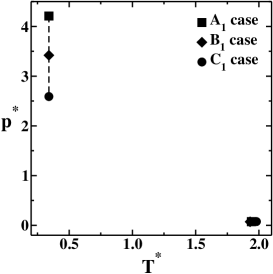
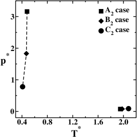
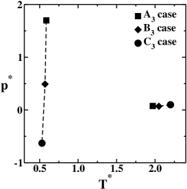
Figure 4: Location of the critical points on pressure-temperature phase diagram for cases $A$, $B$ and $C$.

At very low temperatures the system becomes less diffusive and crystallization might be expected. Here we do not explore all the possible crystal phases, but instead as the temperature is decreased from the liquid phase an amorphous phase is formed. The dotted line in Fig. 3 shows the separation between the fluid phase and the amorphous region. The amorphous phase is identified by the region where the diffusion coefficient becomes zero and the radial distribution functions do not exhibit the periodicity of a solid. Table 6 have the characteristic pressure and temperature values of the amorphous phase boundary for the different models. It shows that the region in the pressure-temperature phase diagram where the amorphous phase is present shrinks as the shoulder part of the potential becomes deeper.

Density Anomaly

Next, we test the effects that the decrease of the distance between the two length scales and the increase of the depth of the first scale have in the presence of the density anomaly. Fig. 3 shows the isochores $0.30\leq\rho^{*}\leq 0.65$ represented by thin solid lines for the nine models. Equation

$$\left(\frac{\partial V}{\partial T}\right)_{p}=-\left(\frac{\partial p}{\partial T}\right)_{V}\left(\frac{\partial V}{\partial p}\right)_{T}$$ (4)

indicates that the temperature of minimum pressure at constant density is the temperature of maximum density at constant pressure, the TMD. The TMD is the boundary of the region of thermodynamic anomaly, where a decrease in the temperature at constant pressure implies an anomalous increase in the density and therefore an anomalous behavior of density (similar to what happens in water). Figs. 3 show the TMD as solid thick lines. For all potentials $A$, $B$ and the potentials $C_{1}$ and $C_{2}$ the TMD is present but for potential $C_{3}$ the TMD is not observed.

Similarly to what happens with the location of amorphous region, as the distance between the shoulder and the attractive scales decreases, the region in the pressure-temperature phase diagram delimited by the TMD line shrinks and disappears for the case $C_{3}$. For the potential $B$ the TMD line is located at temperatures bellow the temperature of the liquid-liquid critical point. The thermodynamic parameters that limits the TMD in phase diagram are shown in the Table 7, where $p_{l}$ represents the values of $(\rho^{*},T^{*},p^{*})$ for the point of the lowest pressure in the TMD line, $p_{m}$ is the point with the highest temperature and $p_{h}$ is the point with the highest pressure.

How can this result be understood? The density anomalous behavior arises from the competition between the two length scales: the shoulder scale and the attractive scale. At high pressures the shoulder scale wins and at low pressures the attractive scale wins. The density anomalous region exists only in the intermediate pressure range where clusters of both scales are present. The value of the “high” pressure and of the “low” pressure is determined by the difference in energy between the two scales. If the difference is too small the low and high pressures are too close and no anomaly appears.

Table 7: Limiting values for density ($\rho^{*}$), temperature ($T^{*}$) and pressure ($p^{*}$) of the thermodynamics anomalies on pressure-temperature diagram. Here the point $p_{l}$ represents the density, temperature and pressure of the point of the lowest pressure in the TMD line, $p_{m}$ represents the point of the highest temperature and $p_{h}$ represents the point of the highest pressure of the TMD line.

cases		$p_{l}$	$p_{m}$	$p_{h}$	cases		$p_{l}$	$p_{m}$	$p_{h}$	cases		$p_{l}$	$p_{m}$	$p_{h}$
	$\rho^{*}$	$0.47$	$0.54$	$0.61$		$\rho^{*}$	$0.47$	$0.52$	$0.57$		$\rho^{*}$	$0.45$	$0.51$	$0.55$
$A_{1}$	$T^{*}$	$0.71$	$1.00$	$0.72$	$B_{1}$	$T^{*}$	$0.71$	$0.85$	$0.69$	$C_{1}$	$T^{*}$	$0.56$	$0.69$	$0.40$
	$p^{*}$	$1.74$	$3.22$	$4.50$		$p^{*}$	$1.50$	$2.50$	$3.30$		$p^{*}$	$0.79$	$1.96$	$2.60$
	$\rho^{*}$	$0.46$	$0.51$	$0.59$		$\rho^{*}$	$0.46$	$0.50$	$0.54$		$\rho^{*}$	$0.46$	$0.48$	$0.50$
$A_{2}$	$T^{*}$	$0.70$	$1.00$	$0.54$	$B_{2}$	$T^{*}$	$0.67$	$0.76$	$0.63$	$C_{2}$	$T^{*}$	$0.49$	$0.53$	$0.48$
	$p^{*}$	$1.36$	$2.20$	$3.17$		$p^{*}$	$0.90$	$1.40$	$1.80$		$p^{*}$	$0.23$	$0.45$	$0.64$
	$\rho^{*}$	$0.45$	$0.48$	$0.54$		$\rho^{*}$	$0.40$	$0.42$	$0.43$		$\rho^{*}$	-	-	-
$A_{3}$	$T^{*}$	$0.66$	$0.89$	$0.69$	$B_{3}$	$T^{*}$	$0.44$	$0.54$	$0.52$	$C_{3}$	$T^{*}$	-	-	-
	$p^{*}$	$0.91$	$1.27$	$1.72$		$p^{*}$	$0.15$	$0.29$	$0.36$		$p^{*}$	-	-	-

Diffusion anomaly

Then, we check the effects that the decrease of the distance between the two scales have in the location in the pressure-temperature phase diagram of the diffusion anomaly. The diffusion coefficient is obtained from the expression:

$$D=\lim_{t\rightarrow\infty}\frac{\langle\left[\vec{r}_{j}(t_{0}+t)-\vec{r}_{j}(t_{0})\right]^{2}\rangle_{t_{0}}}{6t}$$ (5)

where $\vec{r}_{j}(t)$ are the coordinates of particle $j$ at time $t$, and $\langle\cdots\rangle_{t_{0}}$ denotes an average over all particles and over all $t_{0}$.

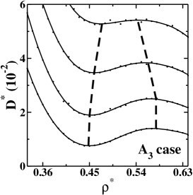
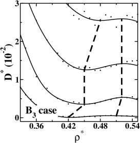
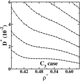
Figure 5: Diffusion coefficient versus reduced density for $T^{*}=0.6,0.7,0.8,0.9$ from the bottom to the top for the case $A_{3}$, $T^{*}=0.4,0.5,0.6,0.7$ from the bottom to the top for the case $B_{3}$ and $T^{*}=0.5,0.6,0.7,0.8,0.9$ from the bottom to the top for the case $C_{3}$. The dots are the simulational data and the solid lines are polynomial fits. The dashed lines connect the densities of minima and maxima diffusivity that limit the diffusion anomalous region.

Fig. 5 shows the behavior of the dimensionless translational diffusion coefficient, $D^{*}$, as function of the dimensionless density, $\rho^{*}$, at constant temperature for the cases. $A_{3}$, $B_{3}$ and $C_{3}$. The solid lines are a polynomial fits to the data obtained by simulation (the dots in the Fig. 5). For normal liquids, the diffusion at constant temperature increases with the decrease of the density. For the cases $A_{1},A_{2},B_{1},B_{2},B_{3},C_{1},C_{2}$ (not shown) and for the cases $A_{3}$ and $B_{3}$ the diffusion has a region in the pressure-temperature phase diagram in which the diffusion increases with density. This is the diffusion anomalous region illustrated in Fig. 3 as a dashed line.

Similarly to what happens with the location of the TMD, as the two length scales becomes closer, the region in the pressure-temperature phase diagram delimited by the extrema of the diffusion goes to lower pressures, shrinks and disappears for the case $C_{3}$.

Fig. 3 illustrates that the region in the pressure-temperature phase diagram where the dynamic anomaly occurs englobes the region where the thermodynamic anomaly is present. This hierarchy between the anomalies is observed in simulations  [57, 35, 34] and in experiments [10] for bulk water.

Structural anomaly

Now, we test the effects that the decrease of the distance between the two length scales have in the location in the pressure-temperature phase diagram of the structural anomalous region.

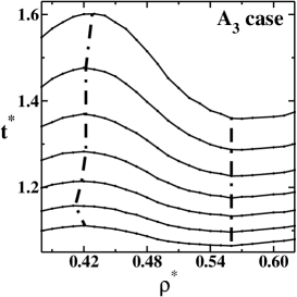
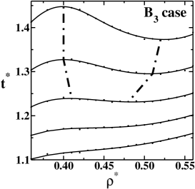
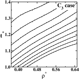
Figure 6: The translational order parameter as a function of density for fixed temperatures: $T^{*}=1.50,\ 1.40,\ 1.30,\ 1.20,\ 1.10,\ 1.00,\ 0.90,\ 0.80,\ 0.70$ and $0.60$ (from top to bottom) for the setting potentials $A$ and $C$; and $T^{*}=1.00,\ 0.90,\ 0.80,\ 0.70$ and $0.60$ for the setting potential $B$. The dot-dashed lines locate the density of maxima e minima $t^{*}$.

The translational order parameter is defined as [29, 35, 72]

$$t=\int_{0}^{\xi_{c}}\left|g(\xi)-1\right|d\xi$$ (6)

where $\xi=r\rho^{\frac{1}{3}}$ is the distance $r$ in units of the mean interparticle separation $\rho^{-\frac{1}{3}}$, $\xi_{c}$ is the cutoff distance set to half of the simulation box times [55] $\rho^{-\frac{1}{3}}$, $g(\xi)$ is the radial distribution function which is proportional to the probability of finding a particle at a distance $\xi$ from a referent particle. The translational order parameter measures how structured is the system. For an ideal gas it is $g=1$ and $t=0$, while for the crystal phase it is $g\neq 1$ over long distances resulting in a large t. Therefore for normal fluids $t$ increases with the increase of the density.

Fig. 6 shows the translational order parameter as a function of the density for fixed temperatures for potentials $A_{3}$, $B_{3}$ and $C_{3}$. The dots represent the simulation data and the solid line the polynomial fit to the data. For the potentials $A_{3}$ and $B_{3}$ there are a region of densities in which the translational parameter decreases as the density increases. A dotted-dashed line illustrates the region of local maximum and minimum of $t^{*}$ limiting the anomalous region. For the potential $C_{3}$, $t^{*}$ increases with the density. No anomalous behavior is observed. The potentials $A_{1},A_{2},B_{1},B_{2},C_{1}$ and $C_{2}$ that do show anomalous behavior are not shown here for simplicity.

Fig. 3 shows the structural anomaly for the families $A$, $B$ and $C$, as dotted-dashed lines. It is observed that the region of structural anomaly embraces both dynamic and thermodynamic anomalies. As the distance between the shoulder and the attractive scales is decreased, the structural anomalous region in the pressure-temperature phase diagram shrinks.

Another measure of the anomalous behavior is the orientational order parameter [73], $Q_{6}$. This parameter is used to get information about tetrahedral order of the molecules. For two length scales spherical symmetric continuous (continuous force) potentials, $Q_{6}$ [55, Al06, 74] exhibit a region of temperatures in which it decreases with increasing density. The maximum of $Q_{6}$ is located in the same region in the pressure temperature phase diagram of the maximum of the translational order parameter [55]. A similar behavior is expected for our potential.

In resume, for all the density, diffusion and structural anomalous regions in the pressure-temperature phase diagram, as the two length scales becomes closer the region of the pressure-temperature phase diagram occupied by the anomalous region shrinks. The same effect is observed when the shoulder scale becomes deeper [18].

Radial distribution function

What is the origin of the disappearance of the thermodynamic, dynamic and structural anomalous behavior with the decrease of the distance between the scales? In order to answer to this question the behavior of the radial distribution function for the nine different potentials is studied. The radial distribution function is a measure of the probability of finding a pair of atoms separated by $r$. This function is defined as

$$g(r)=\frac{V}{N^{2}}\left<\sum_{i,j=1}^{N}\delta\left[\vec{r}-(\vec{r}_{i}(t_{0}+t)-\vec{r}_{j}(t_{0}))\right]\right>_{t_{0}}$$ (7)

where $\vec{r}_{j}(t)$ are the coordinates of particle $i$ and $j$ at time $t$, $V$ is volume of system, $N$ is number of particles and $\langle\cdots\rangle_{t}$ denotes an average over all particles.

Recently it was shown that a necessary condition for the presence of density anomaly is to have particles moving from one scale to the other as the temperature is increased [55, 57, 63], for a fixed density. Here we test if this assumption is confirmed in the potentials we are analyzing. Fig. 7 illustrates the radial distribution function versus distance for a fixed density and various temperatures for the potentials $A_{3}$, $B_{3}$ and $C_{3}$. For the potentials $A_{3}$ and $B_{3}$ the percentage of particles in the first length scale increases while the percentage of particles in the second length scale decreases as the temperature is increased. This means that as the system is heated at constant density particles move from one scale to the other. This behavior is also observed for the potentials $A_{1},A_{2},B_{1},B_{2},C_{1}$ and $C_{2}$ (not shown here for simplicity) and confirms our assumption that the presence of anomalies is related with particles moving from one length scale to the other length scale [55, 57]. This is not the case for the potential $C_{3}$. For the case $C_{3}$, as the temperature is increased the particles move from the second to the other further away coordination shells and the percentage of particles at the first scale is not affected by the increase in temperature and therefore no anomaly is observed [55, 57].

How can we understand this result? The density anomaly appears if particles move from the second length scale to the first length scale. In the case of the potentials $A_{3}$ and $B_{3}$ the difference in energy between the two scales is high and heat is required for having particles reaching the shoulder length scale. Consequently, as the temperature is increased at constant density, more particles will be at the first scale and pressure decreases (see Fig. 7). In the potential $C_{3}$ the difference in energy between the two length scales is small. Almost no heat is required to have particles in the first length scales that saturates. So particles actually do not move from one scale to the other.

This picture in terms of the presence of particles in the different shells can also be checked in the framework of the excess entropy [55, 57].

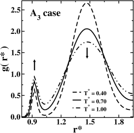
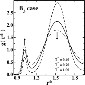
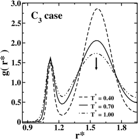
Figure 7: Radial distribution function versus reduced distance for three cases, $A_{3},B_{3},C_{3}$ for reduced density $\rho^{*}=0.480,0.420$ and $0.390$, respectively. In cases $A_{3}$ and $B_{3}$ the first peak of $g(r^{*})$ increases with increasing temperature, while the second peak decreases. In $C_{3}$ case for the first peak potential keeps constant while the second peak decreases.

Excess entropy and anomalies

The excess entropy is defined as the difference between the entropy of the real fluid and that of an ideal gas at the same temperature and density. It also can be given by its two body contribution of $s_{\mathrm{ex}}$,

$$s_{sex}\approx s_{2}=-2\pi\rho\int_{0}^{\infty}{[g(r)\ln g(r)-g(r)+1]r^{2}dr},$$ (8)

gives a good approximation of $s_{sex}$.

What can we learn from the excess entropy about the mechanism responsible for the density, the diffusion and the structural anomalies? In the sec. IV we have shown using the radial distribution function that for potentials that exhibit density, diffusion and structural anomalous behavior as the temperature is increased particles move from the second coordination shell to the first coordination shell. In the case of systems in which no anomalies are present, as the temperature is increased particles will move from the first and second shells to further shells. Therefore, in principle the information about the behavior of particles up to the second coordination shell would be enough to predict if a system would have anomalous behavior.

In order to test this assumption we compute the integrals in the expression for $s_{2}^{(2)}$ (see Eq. (8)) up to the second coordination shell, namely

$$s_{2}^{(2)}=-2\pi\rho\int_{0}^{r_{2}}{[g(r)\ln g(r)-g(r)+1]r^{2}dr},$$ (9)

where $r_{2}$ is the distance of the second shell.

Fig. 8 shows the density dependence of $s_{2}$ along a series of isotherms spanning from $T^{*}=0.60$ to $T^{*}=1.50$ for the cases $A_{3}$, $B_{3}$ and $C_{3}$.

Fig. 9 shows the density dependence of $s_{2}^{(2)}$ along a series of isotherms spanning from $T^{*}=0.60$ to $T^{*}=1.50$ for the cases $A_{3}$, $B_{3}$ and $C_{3}$. The dots are the simulational data and the solid lines are polynomial fits.

Notice that both $s_{2}^{(2)}$ and $s_{2}$ has a maximum and a minimum for the cases $A_{3}$ and $B_{3}$ but not for the case $C_{3}$ what indicates an anomalous behavior in the excess entropy. Comparison between Fig. 8 and Fig. 9 shows that the excess entropy computed up to the second shell not only gives the same trend but also the same density for the maximum and minimum of the excess entropy.

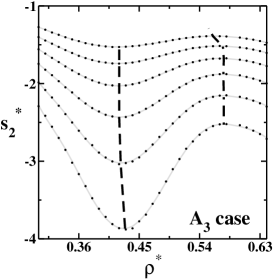
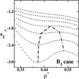
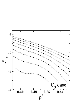
Figure 8: Excess entropy, $s_{2}$, versus reduced density for fixed temperatures $T^{*}=0.6,\,0.7,\,0.8,\,0.9,\,1.0,\,1.1$ from the bottom to the top for the case $A_{3}$, $T^{*}=0.6,\,0.7,\,0.8,\,0.9,\,1.0,\,1.1\,,1.2$ from the bottom to the top for the case $B_{3}$ and temperatures $T^{*}=0.5,\,0.6,\,0.7,\,0.8,\,0.9,\,1.0,\,1.1,\,1.2$ from the bottom to the top for the case $C_{3}$. The temperature $T^{*}=0.5$ contains densities that are metastable points regarding the high density liquid phase. The dot-dashed lines locate the density of maxima $s_{2}$ and the dashed, the minima.

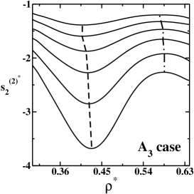
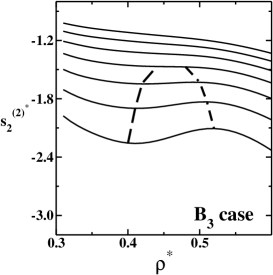
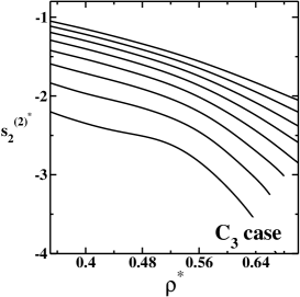
Figure 9: Excess entropy computed up to the second coordination shell, $s_{2}^{2}$, versus reduced density for fixed temperatures $T=0.6,\,0.7,\,0.8,\,0.9,\,1.0,\,1.1$ from the bottom to the top for the case $A_{3}$, $T=0.6,\,0.7,\,0.8,\,0.9,\,1.0,\,1.1,\,1,2$ from the bottom to the top for the $B_{3}$ and temperatures $T=0.5,\,0.6,\,0.7,\,0.8,\,0.9,\,1.0,\,1.1,\,1.2$ from the bottom to the top for the case $C_{3}$. The temperature $T^{*}=0.5$ contains densities that are metastable points regarding the high density liquid phase. The dot-dashed lines locate the density of maxima $s_{2}$ and the dashed, the minima.

Errington et al. have shown that the density anomaly is given by the condition $\Sigma_{\mathrm{ex}}=\left(\partial s_{\mathrm{ex}}/\partial\ln\rho\right)_{T}>1$ [65]. They have also suggested that the diffusion anomaly can be predicted by using the empirical Rosenfeld’s parametrization [75]. Based on Rosenfeld’s scaling parameters and approximating the excess entropy and its derivative by the two body contribution, namely, $s_{\mathrm{ex}}\approx s_{2}$ and $\Sigma_{\mathrm{ex}}=\Sigma_{2}$ the anomalous behavior of the thermodynamic and dynamic quantities are observed if

$$excessentropy \rightarrow {\sum}_{2}\geq 0$$

$$diffusivity \rightarrow {\sum}_{2}\geq 0.42$$

$$viscosity \rightarrow {\sum}_{2}\geq 0.83$$

$$density \rightarrow {\sum}_{2}\geq 1.00\;\;.$$ (10)

This sequence of anomalies is consistent with the studies of Yan et al. [74, 62, 57, 15, 61, 63] where structural anomalies are found to precede diffusivity anomalies, which in turn precede density anomalies.

In order to check these criteria in our family of potentials we compute of $\sum_{2}$ given by:

$${\sum}_{2}=\left(\frac{\partial s_{2}}{\partial\ln\rho}\right)_{T}=s_{2}-2\pi\rho^{2}\int{\ln g(r)\frac{\partial g(r)}{\partial\rho}r^{2}dr}\;.$$ (11)

And also to test if the criteria given by Eq. (10) can also be applied for computations of the excess entropy derivative computed up to the second shell we also calculate

$${\sum}_{2}^{(2)}=\left(\frac{\partial s_{2}}{\partial\ln\rho}\right)_{T}=s_{2}^{(2)}-2\pi\rho^{2}\int_{0}^{r_{2}}{\ln g(r)\frac{\partial g(r)}{\partial\rho}r^{2}dr}$$ (12)

Fig. 10 and Fig. 11 show the behavior of $\sum_{2}$ and of $\sum_{2}^{(2)}$ with the density respectively for a fixed temperature for the potentials $A_{3},B_{3}$ and $C_{3}$. The horizontal lines at $\sum_{2}=0,\ 0.42$ and $1.00$ indicate the threshold beyond which there are structural, diffusion and density anomalies respectively. The graphs confirm that the density, the diffusion and the structural anomalous behavior is observed for the potentials $A_{3}$ and $B_{3}$ but not for the potential $C_{3}$, confirming Errington’s criteria.

The comparison between Fig. 10 and Fig. 11 shows that the derivative of the excess entropy computed up to the second shell is a good approximation for $\sum_{2}$ for all the cases.

This result together with the good agreement between $s_{2}$ and $s_{2}^{(2)}$ supports our surmise that focusing in the first and second shell behavior we can understand the mechanism that leads to the anomalous behavior.

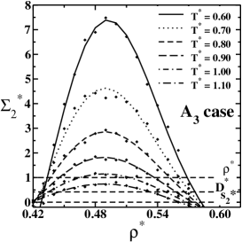
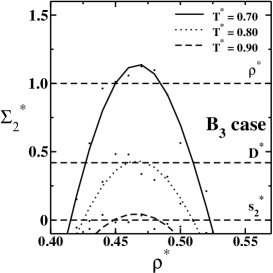
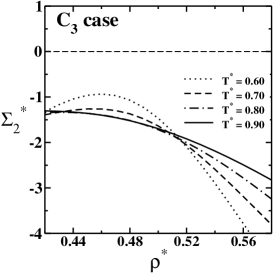
Figure 10: $\sum_{2}^{(2)}$ versus reduced density for temperatures

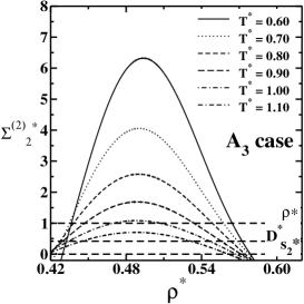
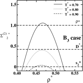
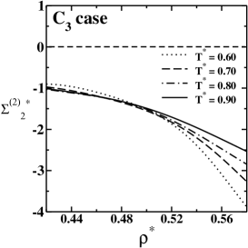
Figure 11: $\sum_{2}^{(2)}$ versus reduced density computed up to the second coordination shell

V Conclusions

In this paper we analyzed three families of potentials characterized by two length scales: a shoulder scale and an attractive scale. We found that when approaching the two scales and keeping the slope between them fixed, the liquid-liquid critical point goes to lower pressures while keeping the critical temperature fixed. This result seems to indicate that the slope of the curve might be related to the critical temperature while the distance between the scales control the critical pressure. This assumption is also supported by another continuous spherical symmetric potential in which the slope was varied [61].

We also found anomalous behavior in the density, in the diffusion coefficient, in the structural order parameter and in the excess entropy for all the cases in which the distance between the scales were not too short.

From the behavior of the radial distribution function we did infer that the anomalies are related to particles moving from one scale to the other.

In order to check our assumption the excess entropy and its derivative were computed in two ways: the total value and the value computed by integrating up to the second coordination shell. We found that the behavior obtained by computing these quantities up to the second coordination shell is accurate both for system with and without anomalies. Since the Rosenfeld’s parametrization [75] is just a lower bound, we can say that it is enough to compute $s_{2}$ and $\sum_{2}$ up to the second shell to know if the anomalies are present or not.

References

- [1] P. C. Hemmer and G. Stell. Phys. Rev. Lett., 24:1284, 1970.
- [2] G. Stell and P. C. Hemmer. J. Chem. Phys., 56:4274, 1972.
- [3] M. Silbert and W.H. Young. Phys. Lett. A, 58:469, 1976.
- [4] E. A. Jagla. Minimum energy configurations of repelling particles in two dimensions. J. Chem. Phys., 110:451, Jan. 1999.
- [5] E. A. Jagla. Core-softened potentials and the anomalous properties of water. J. Chem. Phys., 111:8980, Nov. 1999.
- [6] N. B. Wilding and J. E. Magee. Phase behavior and thermodynamic anomalies of core-softened fluids. Phys. Rev. E, 66:031509, Sep. 2002.
- [7] P. Camp. Phys. Rev. E, 68:061506, 2003.
- [8] P. Vilaseca and G. Franzese. J. Non-Cryst. Sol., 357:419, 2011.
- [9] G. S. Kell. J. Chem. Eng. Data, 20:97, 1975.
- [10] C. A. Angell, E. D. Finch, and P. Bach. J. Chem. Phys., 65:3063, 1976.
- [11] T. Tsuchiya. J. Phys. Soc. Jpn., 60:227, 1991.
- [12] C. A. Angell, R. D. Bressel, M. Hemmatti, E. J. Sare, and J. C. Tucker. Phys. Chem. Chem. Phys., 2:1559, 2000.
- [13] Z. Y. Yan, S. V. Buldyrev, P. Kumar, N. Giovambattista, and H. E. Stanley. Phys. Rev. E, 77:042201, 2008.
- [14] P. Kumar, G. Franzese, and H. E. Stanley. J. Phys.: Cond. Matter, 20:244114, 2008.
- [15] A. B. de Oliveira, G. Franzese, P. A. Netz, and M. C. Barbosa. J. Chem. Phys., 128:064901, 2008.
- [16] A. B. de Oliveira, P. A. Netz, and M. C. Barbosa. Europhys. Lett., 85:36001, 2009.
- [17] S. A. Egorov. J. Chem. Phys., 128:174503, 2008.
- [18] N.M. Barraz Jr., E. Salcedo, and M.C. Barbosa. J. Chem. Phys., 131:094504, 2009.
- [19] R. Waler. Essays of natural experiments. Johnson Reprint, New York, 1964.
- [20] R. J. Speedy and C. A. Angell. Journal of Chem. Phys., 65:851, 1976.
- [21] H KANNO and CA ANGELL. WATER - ANOMALOUS COMPRESSIBILITIES TO 1.9-KBAR AND CORRELATION WITH SUPERCOOLING LIMITS. JOURNAL OF CHEMICAL PHYSICS, 70(9):4008–4016, 1979.
- [22] C. A. Angell, M. Oguni, and W. J. Sichina. J. Phys. Chem., 86:998, 1982.
- [23] E Tombari, C Ferrari, and G Salvetti. Heat capacity anomaly in a large sample of supercooled water. CHEMICAL PHYSICS LETTERS, 300(5-6):749–751, FEB 12 1999.
- [24] H. Thurn and J. Ruska. J. Non-Cryst. Solids, 22:331, 1976.
- [25] Handbook of Chemistry and Physics. CRC Press, Boca Raton, Florida, 65 ed. edition, 1984.
- [26] G. E. Sauer and L. B. Borst. Science, 158:1567, 1967.
- [27] S. J. Kennedy and J. C. Wheeler. J. Chem. Phys., 78:1523, 1983.
- [28] R. Sharma, S. N. Chakraborty, and C. Chakravarty. J. Chem. Phys., 125:204501, 2006.
- [29] M. S. Shell, P. G. Debenedetti, and A. Z. Panagiotopoulos. Phys. Rev. E, 66:011202, 2002.
- [30] P. H. Poole, M. Hemmati, and C. A. Angell. Phys. Rev. Lett., 79:2281, 1997.
- [31] S. Sastry and C. A. Angell. Nature Mater., 2:739, 2003.
- [32] F. X. Prielmeier, E. W. Lang, R. J. Speedy, and H.-D. Lüdemann. Diffusion in supercooled water to 300 mpa. Phys. Rev. Lett., 59:1128, Sep. 1987.
- [33] H. J. C. Berendsen, J. R. Grigera, and T. P. Straatsma. J. Phys. Chem., 91:6269, 1987.
- [34] P. A. Netz, F. W. Starr, H. E. Stanley, and M. C. Barbosa. J. Chem. Phys., 115:344, 2001.
- [35] J. R. Errington and P. G. Debenedetti. Relationship between structural order and the anomalies of liquid water. Nature (London), 409:318, Jan. 2001.
- [36] A. Mudi, C. Chakravarty, and R. Ramaswamy. J. Chem. Phys., 122:104507, 2005.
- [37] J. Mittal, J. R. Errington, and T. M. Truskett. J. Phys. Chem. B, 110:18147, 2006.
- [38] P. A. Netz, F. W. Starr, M. C. Barbosa, and H. E. Stanley. Physica A, 314:470, 2002.
- [39] P. A. Netz, F. W. Starr, M. C. Barbosa, and H. E. Stanley. J. Mol. Liq., 101:159, 2002.
- [40] T. Morishita. Phys. Rev. E, 72:021201, 2005.
- [41] A. Scala, M. R. Sadr-Lahijany, N. Giovambattista, S. V. Buldyrev, and H. E. Stanley. J. Stat. Phys., 100:97, 2000.
- [42] S. V. Buldyrev, G. Franzese, N. Giovambattista, G. Malescio, M. R. Sadr-Lahijany, A. Scala, A. Skibinsky, and H. E. Stanley. Physica A, 304:23, 2002.
- [43] S. V. Buldyrev and H. E. Stanley. Physica A, 330:124, 2003.
- [44] A. Skibinsky, S. V. Buldyrev, G. Franzese, G. Malescio, and H. E. Stanley. Phys. Rev. E, 69:061206, 2005.
- [45] G. Franzese, G. Malescio, A. Skibinsky, S. V. Buldyrev, and H. E. Stanley. Phys. Rev. E, 66:051206, 2002.
- [46] A. Balladares and M. C. Barbosa. J. Phys.: Cond. Matter, 16:8811, 2004.
- [47] A. B. de Oliveira and M. C. Barbosa. J. Phys.: Cond. Matter, 17:399, 2005.
- [48] V. B. Henriques and M. C. Barbosa. Phys. Rev. E, 71:031504, 2005.
- [49] V. B. Henriques, N. Guissoni, M. A. Barbosa, M. Thielo, and M. C. Barbosa. Mol. Phys., 103:3001, 2005.
- [50] E. A. Jagla. Phase behavior of a system of particles with core collapse. Phys. Rev. E, 58:1478, Aug. 1998.
- [51] S. Maruyama, K. Wakabayashi, and M.A. Oguni. Aip Conf. Proceedings, 708:675, 2004.
- [52] R. Kurita and H. Tanaka. Science, 206:845, 2004.
- [53] L. Xu, P. Kumar, S. V. Buldyrev, S.-H. Chen, P. Poole, F. Sciortino, and H. E. Stanley. Proc. Natl. Acad. Sci. U.S.A., 102:16558, 2005.
- [54] A. B. de Oliveira, P. A. Netz, T. Colla, and M. C. Barbosa. J. Chem. Phys., 124:084505, 2006.
- [55] A. B. de Oliveira, P. A. Netz, T. Colla, and M. C. Barbosa. J. Chem. Phys., 125:124503, 2006.
- [56] A. B. de Oliveira, M. C. Barbosa, and P. A. Netz. Physica A, 386:744, 2007.
- [57] A. B. de Oliveira, P. A. Netz, and M. C. Barbosa. Euro. Phys. J. B, 64:48, 2008.
- [58] N. V. Gribova, Y. D. Fomin, D. Frenkel, and V. N. Ryzhov. Phys. Rev. E, 79:051202, 2009.
- [59] E. Lomba, N. G. Almarza, C. Martin, and C. McBride. J. Chem. Phys., 126:244510, 2007.
- [60] G. Franzese, G. Malescio, A. Skibinsky, S. V. Buldyrev, and H. E. Stanley. Nature (London), 409:692, 2001.
- [61] J. da Silva, E. Salcedo, A. B. Oliveira, and M. C. Barbosa. J. Phys. Chem., 133:244506, 2010.
- [62] Z. Yan, S. V. Buldyrev, N. Giovambattista, P. G. Debenedetti, and H. E. Stanley. Phys. Rev. E, 73:051204, 2006.
- [63] P. Vilaseca and G. Franzese. J. Chem. Phys., 133:084507, 2010.
- [64] A. Baranyai and D. J. Evans. Phys. Rev. A, 40:3817, 1989.
- [65] J. R. Errington, T. M. Truskett, and J. Mittal. J. Chem. Phys., 125:244502, 2006.
- [66] S. N. Chakraborty and C. Chakravarty. J. Chem. Phys., 124:014507, 2006.
- [67] T. Head-Gordon and F. H. Stillinger. J. Chem. Phys., 98:3313, 1993.
- [68] F. H. Stillinger and T. Head-Gordon. Phys. Rev. E, 47:2484, 1993.
- [69] P. G. Debenedetti et al. et al. J. Phys. Chem., 95:4540, 1991.
- [70] Z. Yan, S. V. Buldyrev, P. Kumar, N. Giovambattista, P. G. Debenedetti, and H. E. Stanley. Phys. Rev. E, 76:051201, 2007.
- [71] M. P. Allen and D. J. Tildesley. Computer Simulations of Liquids. Claredon Press, Oxford, 1st edition, 1987.
- [72] J. E. Errington, P. G. Debenedetti, and S. Torquato. J. Chem. Phys., 118:2256, 2003.
- [73] P. J. Steinhardt, D. R. Nelson, and M. Ronchetti. Phys. Rev. B, 28:784, 1983.
- [74] Z. Yan, S. V. Buldyrev, N. Giovambattista, and H. E. Stanley. Phys. Rev. Lett., 95:130604, 2005.
- [75] Y. Rosenfeld. J. Phys.: Condens. Matter, 11:5415, 1999.