Dynamic Range Selection in Linear Space

Abstract

Given a set $S$ of $n$ points in the plane, we consider the problem of answering range selection queries on $S$: that is, given an arbitrary $x$-range $Q$ and an integer $k>0$, return the $k$-th smallest $y$-coordinate from the set of points that have $x$-coordinates in $Q$. We present a linear space data structure that maintains a dynamic set of $n$ points in the plane with real coordinates, and supports range selection queries in $O((\lg n/\lg\lg n)^{2})$ time, as well as insertions and deletions in $O((\lg n/\lg\lg n)^{2})$ amortized time. The space usage of this data structure is an $\Theta(\lg n/\lg\lg n)$ factor improvement over the previous best result, while maintaining asymptotically matching query and update times. We also present a succinct data structure that supports range selection queries on a dynamic array of $n$ values drawn from a bounded universe.

1 Introduction

The problem of finding the median value in a data set is a staple problem in computer science, and is given a thorough treatment in modern textbooks [6]. In this paper we study a dynamic data structure variant of this problem in which we are given a set $S$ of $n$ points in the plane. The dynamic range median problem is to construct a data structure to represent $S$ such that we can support range median queries: that is, given an arbitrary range $Q=[x_{1},x_{2}]$, return the median $y$-coordinate from the set of points that have $x$-coordinates in $Q$. Furthermore, the data structure must support insertions of points into, as well as deletions from, the set $S$. We may also generalize our data structure to support range selection queries: that is, given an arbitrary $x$-range $Q=[x_{1},x_{2}]$ and an integer $k>0$, return the $k$-th smallest $y$-coordinate from the set of points that have $x$-coordinates in $Q$.

In addition to being a challenging theoretical problem, the range median and selection problems have several practical applications in the areas of image processing [11], Internet advertising, network traffic analysis, and measuring real-estate prices in a region [12].

In previous work, the data structures designed for the above problems that support queries and updates in polylogarithmic time require superlinear space [5]. In this paper, we focus on designing linear space dynamic range selection data structures, without sacrificing query or update time. We also consider the problem of designing succinct data structures that support range selection queries on a dynamic array of values, drawn from a bounded universe: here “succinct” means that the space occupied by our data structure is close to the information-theoretic lower bound of representing the array of values [15].

1.1 Previous Work

Static Case:

The static range median and selection problems have been studied by many different authors in recent years [3, 17, 12, 21, 22, 9, 10, 4, 5, 16]. In these problems we consider the $n$ points to be in an array: that is, the points have $x$-coordinates $\{1,...,n\}$. We now summarize the upper and lower bounds for the static problem. In the remainder of this paper we assume the word-RAM model of computation with word size $w=\Omega(\lg n)$ bits.

For exact range medians in constant time, there have been several iterations of near-quadratic space data structures [17, 21, 22]. For linear space data structures, Gfeller and Sanders [10] showed that range median queries could be supported in $O(\lg n)$ time, and Gagie et al. [9] showed that selection queries could be supported in $O(\lg\sigma)$ time using a wavelet tree, where $\sigma$ is the number of distinct $y$-coordinates in the set of points. Optimal upper bounds of $O(\lg n/\lg\lg n)$ time for range median queries have since been achieved by Brodal et al. [4, 5], and lower bounds by Jørgensen and Larsen [16]; the latter proved a cell-probe lower bound of $\Omega(\lg n/\lg\lg n)$ time for any static range selection data structure using $O(n\lg^{O(1)}n)$ bits of space. In the case of range selection when $k$ is fixed for all queries, Jørgensen and Larsen proved a cell-probe lower bound of $\Omega(\lg k/\lg\lg n)$ time for any data structure using $O(n\lg^{O(1)}n)$ space [16]. Furthermore, they presented an adaptive data structure for range selection, where $k$ is given at query time, that matches their lower bound, except when $k=2^{o(\lg^{2}\lg n)}$ [16]. Finally, Bose et al. [3] studied the problem of finding approximate range medians. A $c$-approximate median of range $[i..j]$ is a value of rank between $\frac{1}{c}\times\lceil\frac{j-i+1}{2}\rceil$ and $(2-\frac{1}{c})\times\lceil\frac{j-i+1}{2}\rceil$, for $c>1$.

Dynamic Case:

Gfeller and Sanders [10] presented an $O(n\lg n)$ space data structure for the range median problem that supports queries in $O(\lg^{2}n)$ time and insertions and deletions in $O(\lg^{2}n)$ amortized time. Later, Brodal et al. [4, 5] presented an $O(n\lg n/\lg\lg n)$ space data structure for the dynamic range selection problem that answers range queries in $O((\lg n/\lg\lg n)^{2})$ time and insertion and deletions in $O((\lg n/\lg\lg n)^{2})$ amortized time. They also show a reduction from the marked ancestor problem [1] to the dynamic range median problem. This reduction shows that $\Omega(\lg n/\lg\lg n)$ query time is required for any data structure with polylogarithmic update time. Thus, there is still a gap of $\Theta(\lg n/\lg\lg n)$ time between the upper and lower bounds for linear and near linear space data structures.

In the restricted case where the input is a dynamic array $A$ of $n$ values drawn from a bounded universe, $[1,\sigma]$, it is possible to answer range selection queries using a dynamic wavelet tree, such as the succinct dynamic string data structure of He and Munro [HM10]. This data structure uses $nH_{0}(A)+o(n\lg\sigma)+O(w)$ bits of space, the query time is $O(\frac{\lg n\lg\sigma}{\lg\lg n})$, and the update time is $O(\frac{\lg n}{\lg\lg n}(\frac{\lg\sigma}{\lg\lg n}+1))$.

1.2 Our Results

In Section 2, we present a linear space data structure for the dynamic range selection problem that answers queries in $O((\lg n/\lg\lg n)^{2})$ time, and performs updates in $O((\lg n/\lg\lg n)^{2})$ amortized time. This data structure can be used to represent point sets in which the points have real coordinates. In other words, we only assume that the coordinates of the points can be compared in constant time. This improves the space usage of the previous best data structure by a factor of $\Theta(\lg n/\lg\lg n)$ [5], while maintaining query and update time.

In Section 3, we present a succinct data structure that supports range selection queries on a dynamic array $A$ of values drawn from a bounded universe, $[1..\sigma]$. The data structure occupies $nH_{0}(A)+o(n\lg\sigma)+O(w)$ bits, and supports queries in $O(\frac{\lg n}{\lg\lg n}(\frac{\lg\sigma}{\lg\lg\sigma}))$ time, and insertions and deletions in $O(\frac{\lg n}{\lg\lg n}(\frac{\lg\sigma}{\lg\lg\sigma}))$ amortized time. This is a $\Theta(\lg\lg\sigma)$ improvement in query time over the dynamic wavelet tree, and thus closes the space gap between the dynamic wavelet tree solution and that of Brodal et al. [5].

2 Linear Space Data Structure

In this section we describe a linear space data structure for the dynamic range selection problem. Our data structure follows the same general approach as the dynamic data structure of Brodal et al. [5]. However, we make several important changes, and use several other auxiliary data structures, in order to improve the space by a factor of $\Theta(\lg n/\lg\lg n)$.

The main data structure is a weight balanced B-tree [2], $T$, with branching parameter $\Theta(\lg^{\varepsilon_{1}}n)$, for $0<\varepsilon_{1}<1/2$, and leaf parameter $1$. The tree $T$ stores the points in $S$ at its leaves, sorted in non-decreasing order of $y$-coordinate. The height of $T$ is $h_{1}=\Theta(\lg n/\lg\lg n)$ levels, and we assign numbers to the levels starting with level $1$ which contains the root node, down to level $h_{1}$ which contains the leaves of $T$. Inside each internal node $v\in T$, we store the smallest and largest $y$-coordinates in $T(v)$. Using these values we can acquire the path from the root of $T$ to the leaf representing an arbitrary point contained in $S$ in $O(\lg n)$ time; a binary search over the values stored in the children of an arbitrary internal node requires $O(\lg\lg n)$ time per level.

Following Brodal et al. [5], we store a ranking tree $R(v)$ inside each internal node $v\in T$. The purpose of the ranking tree $R(v)$ is to allow us to efficiently make a branching decision in the main tree $T$, at node $v$. Let $T(v)$ denote the subtree rooted at node $v$. The ranking tree $R(v)$ represents all of the points stored in the leaves of $T(v)$, sorted in non-decreasing order of $x$-coordinate. The fundamental difference between our ranking trees, and those of Brodal et al. [5], is that ours are more space efficient. Specifically, in order to achieve linear space, we must ensure that the ranking trees stored in each level of $T$ occupy no more than $O(n\lg\lg n)$ bits in total, since there are $O(\lg n/\lg\lg n)$ levels in $T$. We describe the ranking trees in detail in Section 2.1, but first discuss some auxiliary data structures we require in addition to $T$.

We construct a red-black tree $S_{x}$ that stores the points in $S$ at its leaves, sorted in non-decreasing order of $x$-coordinate. As in [5], we augment the red-black tree $S_{x}$ to store, in each node $v$, the count of how many points are stored in $T(v_{1})$ and $T(v_{2})$, where $v_{1}$ and $v_{2}$ are the two children of $v$. Using these counts, $S_{x}$ can be used to map any query $[x_{1},x_{2}]$ into $r_{1}$, the rank of the successor of $x_{1}$ in $S$, and $r_{2}$, the rank of the predecessor of $x_{2}$ in $S$. These ranking queries, as well as insertions and deletions into $S_{x}$, take $O(\lg n)$ time.

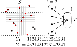
Figure 1: The top two levels of an example tree $T$, and the corresponding strings $Y_{1}$ and $Y_{2}$ for these levels. Each node at level $2$ has exactly $4$ children.

We also store a string $Y(v)$ for each node $v$ in $T$. This string consists of all of the of the points in $T(v)$ sorted in non-decreasing order of $x$-coordinate, where each point is represented by the index of the child of node $v$’s subtree in which they are contained, i.e., an integer bounded by $O(\lg^{\varepsilon_{1}}n)$. However, for technical reasons, instead of storing each string with each node $v\in T$, we concatenate all the strings $Y(v)$ for each node $v$ at level $\ell$ in $T$ into a string of length $n$, denoted by $Y_{\ell}$. Each chunk of string $Y_{\ell}$ from left to right represents some node $v$ in level $\ell$ of $T$ from left to right within the level. See Figure 1 for an illustration. We represent each string $Y_{\ell}$ using the dynamic succinct data structure for representing strings of He and Munro [14]. Depending on the context, we refer to both the string, and also the data structure that represents the string, as $Y_{\ell}$. Consider the following operations on the string $Y_{\ell}$:

• $\mathtt{access}(Y_{\ell},i)$, which returns the $i$-th integer, $Y_{\ell}[i]$, in $Y_{\ell}$;

• $\mathtt{rank}_{\alpha}(Y_{\ell},i)$, which returns the number of occurrences of integer $\alpha$ in $Y_{\ell}[1..i]$;

• $\mathtt{range\_count}(Y_{\ell},x_{1},x_{2},y_{1},y_{2})$, which returns the total number of entries in $Y_{\ell}[x_{1}..x_{2}]$ whose values are in the range $[y_{1}..y_{2}]$;

• $\mathtt{insert}_{\alpha}(Y_{\ell},i)$, which inserts integer $\alpha$ between $Y_{\ell}[i-1]$ and $Y_{\ell}[i]$;

• $\mathtt{delete}(Y_{\ell},i)$, which deletes $Y_{\ell}[i]$ from $Y_{\ell}$.

Let $W=\lceil\frac{\lceil\lg n\rceil^{2}}{\lg\lceil\lg n\rceil}\rceil$. The following lemma summarized the functionality of these data structures for succinct dynamic strings over small universe:

Lemma 1 ([14])

Under the word RAM model with word size $w=\Omega(\lg n)$, a string $Y_{\ell}[1..n]$ of values from a bounded universe $[1..\sigma]$, where $\sigma=O({\lg^{\mu}n})$ for any constant $\mu\in(0,1)$, can be represented using $nH_{0}(Y_{\ell})+O(\frac{n\lg\sigma\lg\lg n}{\sqrt{\lg n}})+O(w)$ bits to support $\mathtt{access}$, $\mathtt{rank}$, $\mathtt{range\_count}$, $\mathtt{insert}$ and $\mathtt{delete}$ in $O(\frac{\lg n}{\lg\lg n})$ time. Furthermore, we can perform a batch of $m$ update operations in $O(m)$ time on a substring $Y_{\ell}[i..i+m-1]$ in which the $j$-th update operation changes the value of $Y_{\ell}[i+j-1]$, provided that $m>\frac{5W}{\lg\sigma}$.

The data structure summarized by the previous lemma is, roughly, a B-tree constructed over the string $Y_{\ell}[1..n]$, in which each leaf stores a superblock, which is a substring of $Y_{\ell}[1..n]$ of length at most $2W$ bits. We mention this because the ranking tree stored in each node of $T$ will implicitly reference to these superblocks instead of storing leaves. Thus, the leaves of the dynamic string at level $\ell$ are shared with the ranking trees stored in nodes at level $\ell$.

As for their functionality, these dynamic string data structures $Y_{\ell}$ are used to translate the ranks $r_{1}$ and $r_{2}$ into ranks within a restricted subset of the points when we navigate a path from the root of $T$ to a leaf. The space occupied by these strings is $O((n\lg(\lg^{\varepsilon_{1}}n)+w)\times\lg n/\lg\lg n)$ bits, which is $O(n)$ words. We present the following lemma:

Lemma 2

Ignoring the ranking trees stored in each node of $T$, the data structures described in this section occupy $O(n)$ words.

In the next section we discuss the technical details of our space-efficient ranking tree. The key idea to avoid using linear space per ranking tree is to not actually store the points in the leaves of the ranking tree, sorted in non-decreasing order of $x$-coordinate. Instead, for each point $p$ in ranking tree $R(v)$, we implicitly reference the the string $Y(v)$, which stores the index of the child of $v$ that contains $p$.

2.1 Space Efficient Ranking Trees

Each ranking tree $R(v)$ is a weight balanced B-tree with branching parameter $\lg^{\varepsilon_{2}}n$, where $0<\varepsilon_{2}<1-\varepsilon_{1}$, and leaf parameter $\Theta(W/\lg\lceil\lg n\rceil)=\Theta((\lg n/\lg\lg n)^{2})$. Thus, $R(v)$ has height $\Theta(\lg n/\lg\lg n)$, and each leaf implicitly represents a substring of $Y(v)$, which is actually stored in one of the dynamic strings, $Y_{\ell}$.

Internal Nodes:

Inside each internal node $u$ in $R(v)$, let $q_{i}$ denote the number of points stored in the subtree rooted at the $i$-th child of $u$, for $1\leq i\leq f_{2}$, where $f_{2}$ is the degree of $u$. We store a searchable partial sums structure [23] for the sequence $Q=\{q_{1},...,q_{f_{2}}\}$. This data structure will allow us to efficiently navigate from the root of $R(v)$ to the leaf containing the point of $x$-coordinate rank $r$. The functionality of this data structure is summarized in the following lemma:

Lemma 3 ([23])

Suppose the word size is $\Omega(\lg n)$. A sequence $Q$ of $O(\lg^{\mu}n)$ nonnegative integers of $O(\lg n)$ bits each, for any constant $\mu\in(0,1)$, can be represented in $O(\lg^{1+\mu}n)$ bits and support the following operations in $O(1)$ time:

• $\mathtt{sum}(Q,i)$ which returns $\sum_{j=1}^{i}Q[j]$,

• $\mathtt{search}(Q,x)$ which returns the smallest $i$ such that $\mathtt{sum}(Q,i)\geq x$,

• $\mathtt{modify}(Q,i,\delta)$ which sets $Q[i]$ to $Q[i]+\delta$, where $|\delta|\leq\lg n$.

This data structure can be constructed in $O(\lg^{\mu}n)$ time, and it requires a precomputed universal table of size $O(n^{\mu^{\prime}})$ bits for any fixed $\mu^{\prime}>0$.

We also store the matrix structure of Brodal et al. [5] in each internal each node $u$ of the ranking tree. Let $f_{1}=\Theta(\lg^{\varepsilon_{1}}n)$ denote the out-degree of node $v\in T$, and let $T(v_{1}),...,T(v_{f_{1}})$ denote the subtrees rooted at the children of $v$ from left to right. Similarly, recall that $f_{2}=\Theta(\lg^{\varepsilon_{2}}n)$ denotes the out-degree of $u\in R(v)$, and let $T^{\prime}(u_{1}),...,T^{\prime}(u_{f_{2}})$ be the subtrees rooted at each child of $u$ from left to right. These matrix structures are a kind of partial sums data structure defined as follows; we use roughly the same notation as [5]:

Definition 1 (Summarizes [5])

A matrix structure $M^{u}$ is an $f_{1}\times f_{2}$ matrix, where entry $M^{u}_{p,q}$ stores the number of points from $\cup_{i=1}^{q}T^{\prime}(u_{i})$ that are contained in $\cup_{i=1}^{p}T(v_{i})$. The matrix structure $M^{u}$ is stored in two ways. The first representation is a standard table, where each entry is stored in $O(\lg n)$ bits. In the second representation, we divide each column into sections of $\Theta(\lg^{1-\varepsilon_{1}}n)$ bits — leaving $\Theta(\lg\lg n)$ bits of overlap between the sections for technical reasons — and we number the sections $s_{1},...,s_{g}$, where $g=\Theta(\lg^{\varepsilon_{1}}n)$. In the second representation, for each column $q$, there is a packed word $w^{u}_{q,i}$, storing section $s_{i}$ of each entry in column $q$. Again, for technical reasons, the most significant bit of each section stored in the packed word $w^{u}_{q,i}$ is padded with a zero bit.

We defer the description of how the matrix structures are used to guide queries until Section 2.2. For now, we just treat these structures as a black box and summarize their properties with the following lemma:

Lemma 4 ([5])

The matrix structure $M^{u}$ for node $u$ in the ranking tree $R(v)$ occupies $O(\lg^{1+\varepsilon_{1}+\varepsilon_{2}}n)$ bits, and can be constructed in $O(\lg^{\varepsilon_{1}+\varepsilon_{2}}n)$ time. Furthermore, consider an update path that goes through node $u$ when we insert a value into or delete a value from $R(v)$. The matrix structures in each node along an update path can be updated in $O(1)$ amortized time per node.

Shared Leaves:

Now that we have described the internal nodes of the ranking tree, we describe the how the leaves are shared between $R(v)$ and the dynamic string over $Y_{\ell}$. To be absolutely explicit, we do not actually store the leaves of $R(v)$: they are only conceptual. We present the following lemma:

Lemma 5

Let $u$ be a leaf in $R(v)$ and $S$ be the substring of $Y(v)$ that $u$ represents, where each value in $S$ is in the range $[1..\sigma]$, and $\sigma=\Theta(\lg^{\varepsilon_{1}}n)$. Using a universal table of size $O(\sqrt{n}\times\mathtt{polylog}(n))$ bits, for any $z\in[1..|S|]$, an array $C_{z}=\{c_{1},...,c_{\sigma}\}$ can be computed in $O(\lg n/\lg\lg n)$ time, where $c_{i}=\mathtt{rank}_{i}(S,z)$, for $1\leq i\leq\sigma$.

Proof

Instead of explicitly storing the leaves of $R(v)$, we use the partial sums structures along the path from the root of $R(v)$ to the parent of leaf $u$ to produce two ranks, $r^{\prime}_{1}$ and $r^{\prime}_{2}$, which are the starting and ending ranks of the substring $S$ represented by $u$ in $Y_{\ell}$. Based on the leaf parameter of $R(v)$, and the properties of weight balanced B-trees [2], $S$ can have length $\Theta(W/\lg\lg n)$. Following the analysis of how superblocks are laid out in the dynamic string $Y_{\ell}$, this means that $S$ is stored in a constant number of consecutive superblocks [13, Section 4].

Given that we know $r^{\prime}_{1}$ and $r^{\prime}_{2}$, we can acquire a pointer to the first superblock that stores part of $S$ in $O(\lg n/\lg\lg n)$ time [13, Lemma 7]. Inside each superblock the substring is further decomposed into a list of blocks of length $O((\lg n)^{3/2})$ bits each, in which only the final block has free space. In order to produce the array $C_{z}$, we scan the list of blocks in the superblock up to position $z$, reading $(\lg n)/2$ bits at a time. Since each value in $[1..\sigma]$ occupies $\varepsilon_{1}\lg\lg n$ bits, we can read $\Theta(\lg n/\lg\lg n)$ values at a time. As we read these values, we keep a running total of the ranks of each value in $[1..\sigma]$ up to our current position. Let field $b_{i}$ denote $\mathtt{rank}_{i}(S,p)$, where $p$ is our current position within $S$. Clearly, $b_{i}$ occupies $O(\lg\lg n)$ bits. Furthermore, let $b=b_{1}...b_{\sigma}$ be the concatenation of these fields. Thus, the running total, $b$, contains at most $2\lg^{\varepsilon_{1}}\times\varepsilon_{1}\lg\lg n$ bits, and can be stored in a constant number of words.

In order to efficiently update our running total $b$ after reading a $(\lg n)/2$ bits from the current block, we perform a lookup in a universal table $A$. Let $a$ denote the $a$-th lexicographically smallest string of length $(\lg n)/2$ bits, over the bounded universe $[1,\sigma]$. Also, let $f_{i}(a)$ denote the frequency of symbol $i\in[1,\sigma]$ in string $a$. In each entry of the table $A[a]$, we store the value $b^{\prime}=f_{1}(a)...f_{\sigma}(a)$. Since both $b$ and $b^{\prime}$ fit in a constant number of words, we can exploit word-level parallelism to update the running total by summing all the fields in $b$ and $b^{\prime}$ in $O(1)$ time.

The table $A$ occupies $O(2^{(\lg n)/2}\times\lg^{\varepsilon_{1}}n\times\lg\lg n)=O(\sqrt{n}\times\mathtt{polylog}(n))$ bits, and allows us to process $\Theta(\lg n/\lg\lg n)$ values in $O(1)$ time. Recall that the entire superblock contains $\Theta((\lg n/\lg\lg n)^{2})$ values. Thus, we can return $C_{z}$ in $O((\lg n/\lg\lg n)^{2}\times(\lg\lg n/\lg n))$ time.

We now present the following lemma regarding the space and construction time of the ranking trees:

Lemma 6

Each ranking tree $R(v)$ occupies $O\left(\frac{m(\lg\lg n)^{2}}{\lg^{1-\varepsilon_{1}}n}+w\right)$ bits of space if $|T(v)|=m$, and requires $O(m)$ time to construct, assuming that we have access to the string $Y(v)$.

Proof

The space occupied by the internal nodes is $O(m(\lg\lg n)^{2}/\lg^{1-\varepsilon_{1}}n)$ bits, since each internal node occupies $O(\lg^{1+\varepsilon_{1}+\varepsilon_{2}}n)$ bits by Lemmas 3 and 4, and the number of internal nodes is $O(m/\lg^{\varepsilon_{2}}n\times(\lg\lg n/\lg n)^{2})$. In order to reduce the cost of the pointers between the internal nodes in $R(v)$ to $O(\lg n)$ bits per pointer, we make use of well known memory blocking techniques for dynamic data structures (e.g., see [13, Appendix J]). The main idea is to allocate a fixed memory area for the entire ranking tree, and perform all updates to the ranking tree using memory from this area. After $\Theta(m)$ updates, we allocate a new area and copy over the entire ranking tree. The cost of using this memory blocking will amount to $O(1)$ amortized time per update. Thus the overall space is $O(m(\lg\lg n)^{2}/\lg^{1-\varepsilon_{1}}n+w)$ bits, since we must count the pointer to the root of the ranking tree, stored at the start of the fixed memory area.

Now we analyze the overall construction time. Based on Lemmas 3 and 4, we can construct all the internal nodes in $O(m)$ time, since the number of internal nodes is $O(m/\lg^{\varepsilon_{2}}\times(\lg\lg n/\lg n)^{2})$, and each requires $o(\lg^{1+\varepsilon_{1}+\varepsilon_{2}}n)+O(\lg^{\varepsilon_{2}}n)$ time to construct.

Remark 1

Note that the discussion in this section implies that we need not store ranking trees for nodes $v\in T$, where $|T(v)|=O(\lg n/\lg\lg n)^{2}$. Instead, we can directly query the dynamic string $Y_{\ell}$ using Lemma 5 in $O(\lg n/\lg\lg n)$ time to make a branching decision in $T$. This will be important in Section 3, since it significantly reduces the number of pointers we need.

2.2 Answering Queries

In this section, we explain how to use our space efficient ranking tree in order to guide a range selection query in $T$.

We are given a query $[x_{1},x_{2}]$ as well as a rank $k$, and our goal is to return the $k$-th smallest $y$-coordinate in the query range. We begin our search at the root node $v$ of the tree $T$. In order to guide the search to the correct child of $v$, we determine the canonical set of nodes in $R(v)$ that represent the query $[x_{1},x_{2}]$. Before we query $R(v)$, we search for $x_{1}$ and $x_{2}$ in $S_{x}$. Let $r_{1}$ and $r_{2}$ denote the ranks of the successor of $x_{1}$ and predecessor of $x_{2}$ in $S$, respectively. We query $R(v)$ using $[r_{1},r_{2}]$, and use the searchable partial sum data structures stored in each node of $R(v)$, to identify the canonical set of nodes in $R(v)$ that represent the interval $[r_{1},r_{2}]$. At this point we outline how to use the matrix structures in order to decide how to branch in $T$.

Matrix Structures:

We discuss a straightforward, slow method of computing the branch of the child of $v$ to follow. We then discuss the details of a faster method, which can also be found in the original paper [5].

In order to determine the child of $v$ that contains the $k$-th smallest $y$-coordinate in the query range, recall that $T$ is sorted by $y$-coordinate. Let $f_{1}$ denote the degree of $v$, and $q^{\prime}_{i}$ denote the number of points that are contained in the range $[x_{1},x_{2}]$ in the subtree rooted at the $i$-th child of $v$, for $1\leq i\leq d$. Determining the child that contains the $k$-th smallest $y$-coordinate in $[x_{1},x_{2}]$ is equivalent to computing the value $\tau$ such that $\sum_{i=1}^{\tau-1}q^{\prime}_{i}<k$ and $\sum_{i=1}^{\tau}q^{\prime}_{i}\geq k$. In order to compute $\tau$, we use the matrix structures in each internal node of the canonical set of nodes, $C$, that represent $[x_{1},x_{2}]$. The set $C$ contains $O(\lg n/\lg\lg n)$ internal nodes, as well as at most two leaf nodes.

Consider any internal node $u\in C$, and without loss of generality, suppose $u$ was on the search path for $r_{1}$, but not the search path for $r_{2}$, and that $u$ has degree $f_{2}$. If the search path for $r_{1}$ goes through child $c_{q}$ in $u$, then consider the difference between columns $f_{2}$ and $q$ in the first representation of matrix $M^{u}$. We denote this difference as $M^{\prime u}$, where $M^{\prime u}_{i}=M^{u}_{i,f_{2}}-M^{u}_{i,q}$, for $1\leq i\leq f_{1}$. For each internal node $u\in C$ we add each $M^{\prime u}$ to a running total, and denote the overall sum as $M^{\prime}$. Next, for each of the — at most — two leaves on the search path, we query the superblocks of $Y_{\ell}$ to get the relevant portions of the sums, and add them to $M^{\prime}$. At this point, $M^{\prime}_{i}=q^{\prime}_{i}$, and it is a simple matter to scan each entry in $M^{\prime}$ to determine the value of $\tau$. Since each matrix structure has $f_{1}$ entries in its columns, this overall process takes $O(f_{1}\times\lg n/\lg\lg n)=O(\lg^{1+\varepsilon_{1}}n/\lg\lg n)$ time, since there are $O(\lg n/\lg\lg n)$ levels in $R(v)$. Since there are $O(\lg n/\lg\lg n)$ levels in $T$, this costs $O((\lg n/\lg\lg n)^{2}\times\lg^{\varepsilon_{1}}n)$ time. This time bound can be reduced by a factor of $f_{1}=O(\lg^{\varepsilon_{1}}n)$, using a slightly faster method which we now describe.

Faster method:

The main idea of the fast method is to use word-level parallelism and the second representation of each matrix in order to speed up the query time. When we begin our search in the root node $v$ of the tree $T$, consider the sections of $k$, denoted $k_{1},...,k_{g}$. We query $R(v)$, using the first section $k_{1}$ to guide the search. In order to remove the $f_{1}$ factor from the slow method, in each internal node $u$ we subtract the packed words $w^{u}_{1,f_{2}}-w^{u}_{1,q}$, then add them to a running total $w_{1}$. After we have summed the differences between the packed words in all the internal nodes, we add the relevant sections from the canonical leaf nodes using Lemma 5.

Since $w_{1}$ is only a rough approximation of the first section of $M^{\prime}$, each value in the packed word might be off by $O(\lg n/\lg\lg n)$: the number of additions and subtractions we used to compute $w_{1}$. This means there may be errors, caused by carry bits, in possibly the $O(\lg\lg n)$ least significant bits in each value stored in the packed word $w_{1}$. We scan each entry in $w_{1}$ to determine the indices of the first and last entries in $w_{1}$ that match $k_{1}$, except for the last $O(\lg\lg n)$ bits , as well as the first value that is greater than $k_{1}$ in a more significant bit beyond the $O(\lg\lg n)$ least significant bits. Let $K=\{e_{1},...,e_{b}\}$ denote this set of entries in the packed word $w_{1}$.

Next, we check the largest and smallest entries, $e_{1}$ and $e_{b}$, in $K$ in order to determine if one of these is $\tau$. This can be done in $O(\lg n/\lg\lg n)$ time. If neither $e_{1}$ or $e_{b}$ is $\tau$, then there are several cases for how to proceed. If there are only a constant number of values in $K$, then we can compute the index, $\tau$, of the child of $v$ that we should branch to, by computing the entries in $M^{\prime}$ for these values in $O(\lg n/\lg\lg n)$ time each. We call this the good case. However, if there are a non-constant number of entries in $K$, then we are in the bad case, and we must do a binary search over $M^{\prime}$ to determine $\tau$. This costs $O(\lg\lg n\times\lg n/\lg\lg n)=O(\lg n)$ time in total.

The key observation, is that after we do the binary search for $\tau$ in the bad case, at no point in the future will we ever have to examine the first section of $k$ or the matrix structures. This is because when we are in the bad case, the difference between the first sections of $q^{\prime}_{\tau+1}$ and $q^{\prime}_{\tau}$ is a value that can be stored in $\Theta(\lg\lg n)$ bits: which is why the overlap between sections was set to be $\Theta(\lg\lg n)$. Moreover, since there are only $g=O(\lg^{\varepsilon_{1}}n)$ sections, we can spend at most $O((\lg n)/g\times\lg n)=o((\lg n/\lg\lg n)^{2})$ time in bad cases before we have exhausted all of the bits in the matrix structures; once there are no more bits, we are guaranteed to have found the $k$-th smallest $y$-coordinate in the query range. Since the good case requires $O(\lg n/\lg\lg n)$ time, and there are $O(\lg n/\lg\lg n)$ levels in $T$, our search costs at most $O((\lg n/\lg\lg n)^{2})$ time.

Recursively Searching in $T$:

Let $v_{\tau}$ denote the $\tau$-th child of $v$. The final detail to discuss is how we translate the ranks $[r_{1},r_{2}]$ into ranks in the tree $R(v_{\tau})$. To do this, we query the string $Y(v)$ before recursing to $v_{\tau}$. We use two cases to describe how to find $Y(v)$ within $Y_{\ell}$. In the first case, if $v$ is the root of $T$, then $Y_{\ell}=Y(v)$. Otherwise, suppose the range in $Y_{\ell-1}$ that stores the parent $v_{p}$ of node $v$ begins at position $z$, and $v$ is the $i$-th child of $v_{p}$. Let $c_{j}=\mathtt{range\_count}(Y(v),z,z+|Y(v)|,1,j)$ for $1\leq j\leq f_{1}$. Then, the range in $Y_{\ell}$ that stores $Y(v)$ is $[z+c_{i-1},z+c_{i}]$. We then query $Y(v)$, and set $r_{1}=\mathtt{rank}_{\tau}(Y(v),r_{1})$, $r_{2}=\mathtt{rank}_{\tau}(Y(v),r_{2})$, $k=k-q^{\prime}_{\tau-1}$, and recurse to $v_{\tau}$. We present the following lemma, summarizing the arguments presented thus far:

Lemma 7

The data structures described in this section allow us to answer range selection queries in $O((\lg n/\lg\lg n)^{2})$ time.

2.3 Handling Updates

In this section, we describe the algorithm for updating the data structures. We start by describing how insertions are performed. First, we insert $p$ into $S_{x}$ and look up the rank, $r_{x}$, of $p$’s $x$-coordinate in $S_{x}$. Next, we use the values stored in each internal node in $T$ to find $p$’s predecessor by $y$-coordinate, $p^{\prime}$. We update the path from $p^{\prime}$ to the root of $T$. If a node $v$ on this path splits, we must rebuild the ranking tree in the parent node $v_{p}$ at level $\ell$, as well as the dynamic string $Y_{\ell}$.

Next, we update $T$ in a top-down manner; starting from the root of $T$ and following the path to the leaf storing $p$. Suppose that at some arbitrary node $v$ in this path, the path branches to the $j$-th child of $v$, which we denote $v_{j}$. We insert the symbol $j$ into its appropriate position in $Y_{\ell}$. After updating $Y_{\ell}$ — its leaves in particular — we insert the symbol $j$ into the ranking tree $R(v)$, at position $r_{x}$, where $r_{x}$ is the rank of the $x$-coordinate of $p$ among the points in $T(v)$. As in $T$, each time a node splits in $R(v)$, we must rebuild the data structures in the parent node. We then update the nodes along the update path in $R(v)$ in a top-down manner: each update in $R(v)$ must be processed by all of the auxiliary data structures in each node along the update path. Thus, in each internal node, we must update the searchable partial sums data structures, as well as the matrix structures.

After updating the structures at level $\ell$, we use $Y_{\ell}$ to map $r_{x}$ to its appropriate rank by $x$-coordinate in $T(v_{j})$. At this point, we can recurse to $v_{j}$. In the case of deletions, we follow the convention of Brodal et al. [5] and use node marking, and rebuild the entire data structure after $\Theta(n)$ updates. We present the following theorem:

Theorem 2.1

Given a set $S$ of points in the plane, there is a linear space dynamic data structure representing $S$ that supports range selection queries for any range $[x_{1},x_{2}]$ in $O((\lg n/\lg\lg n)^{2})$ time, and supports insertions and deletions in $O((\lg n/\lg\lg n)^{2})$ amortized time.

Proof

The query time follows from Lemma 7 and the space from Lemmas 2 and 6. All that remains is to analyze the update time.

We can insert a point $p$ into $S_{x}$ in $O(\lg n)$ time. The node structure of $T$ can be updated in $O(\lg^{\varepsilon_{1}}n)$ amortized time by the properties of weight balanced B-trees. Similarly, the node structure of $R(v)$ for each node $v$ in the update path in $T$ can be updated in $O(\lg^{\varepsilon_{2}}n)$ amortized time, and there are $O(\lg n/\lg\lg n)$ ranking trees that are updated. Thus, the tree structure of $T$ and the ranking trees in each node can be updated in $o((\lg n/\lg\lg n)^{2})$ time.

The difficulty arises when a node $v$ in $T$ splits, since the index of $v$ relative to the other children of $v_{p}$ has changed. In this case, we are required to not only rebuild $R(v_{p})$, but also the substring of $Y_{\ell}$ that stores $Y(v_{p})$. If $T(v)$ contains $m$ points, then $Y(v_{p})$ is a string of length $O(m\times\lg^{\varepsilon_{1}}n)$, and constructing $R(v_{p})$ takes $O(\lg^{\varepsilon_{1}}n\times m)$ time after $O(m)$ updates, by Lemma 6. This is $O(\lg^{\varepsilon_{1}}n\times\lg n/\lg\lg n)$ amortized time in total, since splits can occur in each level of $T$.

One issue is that this analysis assumes that we have access to the updated version of $Y(v_{p})$, storing the indices of the children of $v_{p}$, sorted by $x$-coordinate, after the split. We now explain the technical details of how to compute this string; a task that requires a few more definitions. Let $v_{1}$ and $v_{2}$ denote the two nodes into which $v$ splits, and let $c_{1},...,c_{f}$, where $f\in\Theta(\lg^{\varepsilon_{1}}n)$ is the degree of $v$, denote the left-to-right sequence of children of $v$ before the split. Suppose that after the split, children $c_{1},...,c_{d}$ become the children of $v_{1}$ and $c_{d+1},...,c_{f}$ become the children of $v_{2}$, where $1\leq d\leq f$, and $d=\Theta(\lg^{\varepsilon_{1}}n)$. Also suppose that $v$ is the $i$-th child of $v_{p}$, and denote the degree of $v_{p}$ as $f_{p}$.

First, we extract the strings $Y(v_{p})$ and $Y(v)$ from $Y_{\ell}$ and $Y_{\ell+1}$: this requires $O(m\lg^{\varepsilon_{1}}n+\lg n/\lg\lg n)$ time in total, since we must traverse a root-to-leaf path in the dynamic strings. The next step is to scan both strings $Y(v_{p})$ and $Y(v)$ together, and at the same time write an updated string $Y^{\prime}(v_{p})$, which will be the sequence of indices of $v_{p}$’s children, after $v$ is split. When we encounter the index $c$ in $Y(v_{p})$, we append $c$ to $Y^{\prime}(v_{p})$ if $c\in\{1,...,i-1\}$, and $c+1$ if $c\in\{i+1,...,f_{p}\}$. In the case when $c=i$, then we check the corresponding index $c^{\prime}$ in $Y(v)$: if $c^{\prime}\in\{1,...,d\}$, then we append $c$ to $Y^{\prime}(v_{p})$, and a $c+1$ otherwise. For example, let $Y(v)=\{1,2,3,4,1\}$, $Y(v_{p})=\{1,3,3,2,4,1,2,3,3,4,3,1\}$, and $v$ be the $3$-rd child of $v_{p}$. Suppose that $v$ is to be split so that children $1$ and $2$ become the children of $v_{1}$ and $3$ and $4$ become the children of $v_{2}$. Then, following the steps we just described, $Y^{\prime}(v_{p})=\{1,3,3,2,5,1,2,4,4,5,3,1\}$. Overall, generating $Y^{\prime}(v_{p})$ takes $O(m\lg^{\varepsilon_{1}}n+\lg n/\lg\lg n)$ time, since we do one scan through both $Y(v_{p})$ and $Y(v)$. The additive $O(\lg n/\lg\lg n)$ term is absorbed in all but a constant number of levels near the bottom of $T$, where $m=o(\lg^{1-\varepsilon_{1}}n/\lg\lg n)$. Thus, the string generation algorithm described above requires $O(\lg^{\varepsilon_{1}}n\times\lg n/\lg\lg n)$ amortized time, when we consider that each level in $T$ can split during an insertion.

When a split occurs in $T$, we must also do a batched update on the dynamic string $Y_{\ell}$, where $\ell$ is the level of $v_{p}$. To do this, we make use of the batched insertion operation from Lemma 1. When $|T(v_{p})|>5W/\Theta(\lg\lg n)$, where $W$ is the value in Lemma 1, we can replace the $O(m\lg^{\varepsilon_{1}}n)$ values representing $Y(v_{p})$ with $Y^{\prime}(v_{p})$ in $O(m\lg^{\varepsilon_{1}}n)$ time. However, in the alternative case, when $|T(v_{p})|$ is small, we just directly insert and delete values into $Y_{\ell}$ in $O(\lg n/\lg\lg n)$ time per operation. As with the string generation algorithm, the case where $|T(v_{p})|$ is too small for batched updates only occurs in a constant number of bottom levels of $T$. Thus, the overall cost for updating $Y_{\ell}$ for every level in $T$ in which a node is split takes $O(\lg^{\varepsilon_{1}}n\times\lg n/\lg\lg n)$ amortized time.

Finally, we consider the more common case where $v$ does not split during the insertion, and how to update $R(v)$. Consider the update path in $R(v)$, and an arbitrary node $u$ on this path. We can update the searchable partial sums structure in $u$ in $O(1)$ time in the worst case by Lemma 3. If $u$ is split, then the cost of rebuilding the searchable partial sums structure is absorbed by the cost of rebuilding $u$. The matrix structures can be rebuilt in $O(1)$ amortized time per internal node on the update path by Lemma 4, or $O(\lg n/\lg\lg n)$ amortized time per ranking tree. Each conceptual leaf in $R(v)$ takes $O(\lg n/\lg\lg n)$ time to update by Lemma 1 — since we must update the dynamic string — but there are at most two leaves updated per ranking tree. Overall we get that the cost of each update is $O((\lg n/\lg\lg n)^{2})$ amortized time.

3 Dynamic Arrays

In this section, we show how to adapt Theorem 2.1 for problem of maintaining a dynamic array $A$ of values drawn from a bounded universe $[1..\sigma]$. A query consists of a range in the array, $[i..j]$, along with an integer $k>0$, and the output is the $k$-th smallest value in the subarray $A[i..j]$. Inserting a value into position $i$ shifts the position of the values in positions $A[i..n]$ to $A[i+1..n+1]$, and deletions are analogous. We present the following theorem:

Theorem 3.1

Given an array $A[1..n]$ of values drawn from a bounded universe $[1..\sigma]$, there is an $nH_{0}(A)+o(n\lg\sigma)+O(w)$ bit data structure that can support range selection queries on $A$ in $O(\frac{\lg n}{\lg\lg n}\frac{\lg\sigma}{\lg\lg\sigma})$ time, and insertions into, and deletions from, $A$ in $O(\frac{\lg n}{\lg\lg n}\frac{\lg\sigma}{\lg\lg\sigma})$ amortized time.

Proof

The data structure is roughly the same as the tree $T$ from Theorem 2.1, except that now we need a few extra techniques to avoid paying for more than a constant number of pointers. The first idea is to use a generalized wavelet tree $T^{\prime}$ with fan out $O(\lg^{\varepsilon_{1}}\sigma)$ over the universe $[1..\sigma]$, instead of the original weight balanced B-tree $T$, (c.f., Ferragina et al. [7]). The tree $T^{\prime}$ has height $\Theta(\lg\sigma/\lg\lg\sigma)$, and, as in the tree $T$, we store dynamic strings $Y_{\ell}$ at each level in $T^{\prime}$, as well as ranking trees for each node of $T^{\prime}$. The reason we cannot afford to increase the branching factor beyond $\Theta(\lg^{\varepsilon_{1}}\sigma)$ is that the cost of a search in the ranking tree during a bad case (see the description of the faster method from Section 2.2) would dominate the query cost: if the fan out of $T^{\prime}$ is $f^{\prime}$, then the total time in bad cases can be $O((f^{\prime}\lg f^{\prime}\lg n)/\lg\lg n)$.

Another issue is that the pointers to the ranking trees stored in each node of $T^{\prime}$ occupy too much space: the lowest level in $T^{\prime}$ in which we store ranking trees has $O(n(\lg\lg n)^{2}/(\lg^{2}n\lg^{\varepsilon_{1}}\sigma))$ nodes, and therefore $O(nw(\lg\lg n)^{2}/(\lg^{2}n\lg^{\varepsilon_{1}}\sigma))$ bits are required for pointers to the roots of the ranking trees. However, since the maximum number of bits occupied by ranking trees at any level is at most $O\left(n(\lg\lg n)^{2}\lg^{\varepsilon_{1}}\sigma/\lg n\right)$, which is $o(n)$ — not counting the pointers to their roots — we can use the same technique as in Lemma 6 and group all the ranking trees at a given level in $T^{\prime}$ into a fixed memory area of size $o(n)$. Thus, we can replace all of the $O(w)$ bit pointers to the roots of the ranking trees with $O(\lg n)$ bit pointers, and the space for pointers to the ranking trees becomes $o(n)+O(w\lg\sigma/\lg\lg\sigma)$: one pointer to the fixed memory area per level in the tree. We also need $O(w\lg\sigma/\lg\lg\sigma)$ bits to store the pointers to the dynamic strings at each level. At this point, we can use the technique of Mäkinen and Navarro [19] to further reduce this to $O(w)$ bits.

Finally, since we are working solely with ranks rather than $x$-coordinates, we can discard the red-black tree $S_{x}$. To analyze the total space cost we sum the space required by the dynamic strings and the ranking trees at each level in $T$. Thus, the total number of bits required is:

$$\sum_{\ell=1}^{h_{1}}\left(nH_{0}(Y_{\ell})+O\left(\frac{n\lg\lg\sigma(\lg\lg n)^{2}}{\sqrt{\lg n}}+\frac{n(\lg\lg n)^{2}\lg^{\varepsilon_{1}}\sigma}{\lg n}\right)\right)+O(w)$$

By the same arguments presented in [7], this simplifies to:

$$nH_{0}(A)+O\left(\frac{n\lg\sigma(\lg\lg n)^{2}}{\sqrt{\lg n}}\right)+O(w)$$

4 Concluding Remarks

In the same manner as Brodal et al. [5], the data structure we presented can also support orthogonal range counting queries in the same time bound as range selection queries. We note that the cell-probe lower bounds for the static range median and static orthogonal range counting match [20, 16], and — very recently — dynamic weighted orthogonal range counting was shown to have a cell-probe lower bound of $\Omega((\lg n/\lg\lg n)^{2})$ query time for any data structure with polylogarithmic update time [18]. In light of these bounds, it is likely that $O((\lg n/\lg\lg n)^{2})$ time for range median queries is optimal for linear space data structures with polylogarithmic update time. However, it may be possible to do better in the case of dynamic range selection, when $k=o(n^{\varepsilon})$, for any $\varepsilon>0$, using an adaptive data structure as in the static case [16].

Acknowledgements:

We would like to thank Gelin Zhou for pointing out an error in the preliminary version, in the proof of Theorem 2.

References

- [1] Alstrup, S., Husfeldt, T., Rauhe, T.: Marked ancestor problems. In: Proc. 39th Annual Symposium on Foundations of Computer Science. pp. 534–543. IEEE (1998)
- [2] Arge, L., Vitter, J.S.: Optimal external memory interval management. SIAM J. Comput. 32(6), 1488–1508 (2003)
- [3] Bose, P., Kranakis, E., Morin, P., Tang, Y.: Approximate range mode and range median queries. In: Proc. STACS. LNCS, vol. 3404, pp. 377–388. Springer (2005)
- [4] Brodal, G., Jørgensen, A.: Data structures for range median queries. In: Proc. ISAAC. LNCS, vol. 5878, pp. 822–831. Springer (2009)
- [5] Brodal, G., Gfeller, B., Jorgensen, A., Sanders, P.: Towards optimal range medians. Theoretical Computer Science (2010)
- [6] Cormen, T.H., Stein, C., Rivest, R.L., Leiserson, C.E.: Introduction to Algorithms. McGraw-Hill Higher Education, 2nd edn. (2001)
- [7] Ferragina, P., Manzini, G., Mäkinen, V., Navarro, G.: An alphabet-friendly FM-index. In: Proc. SPIRE. pp. 228–228. Springer (2004)
- [8] Fredman, M., Saks, M.: The cell probe complexity of dynamic data structures. In: Proc. STOC. pp. 345–354. ACM (1989)
- [9] Gagie, T., Puglisi, S., Turpin, A.: Range quantile queries: Another virtue of wavelet trees. In: String Processing and Information Retrieval. pp. 1–6. Springer (2009)
- [10] Gfeller, B., Sanders, P.: Towards optimal range medians. In: Proc. ICALP. LNCS, vol. 5555, pp. 475–486. Springer (2009)
- [11] Gil, J., Werman, M.: Computing 2-d min, median, and max filters. IEEE Transactions on Pattern Analysis and Machine Intelligence 15(5), 504–507 (1993)
- [12] Har-Peled, S., Muthukrishnan, S.: Range medians. In: Proc. of the European Symposium on Algorithms. LNCS, vol. 5193, pp. 503–514. Springer (2008)
- [13] He, M., Munro, J.: Succinct representations of dynamic strings. In: Proc. SPIRE. pp. 334–346. Springer (2010), Appendices in Arxiv preprint arXiv:1005.4652
- [14] He, M., Munro, J.I.: Space Efficient Data Structures for Dynamic Orthogonal Range Counting. In: Proc. WADS. LNCS, Springer (2011), to appear
- [15] Jacobson, G.: Space-efficient static trees and graphs. In: Proc. SFCS. pp. 549–554 (1989)
- [16] Jørgensen, A., Larsen, K.: Range selection and median: Tight cell probe lower bounds and adaptive data structures. In: Proc. SODA (2011)
- [17] Krizanc, D., Morin, P., Smid, M.: Range mode and range median queries on lists and trees. Nordic Journal of Computing 12, 1–17 (2005)
- [18] Larsen, K.: The cell probe complexity of dynamic range counting. Arxiv preprint arXiv:1105.5933 (2011)
- [19] Mäkinen, V., Navarro, G.: Dynamic entropy-compressed sequences and full-text indexes. In: Combinatorial Pattern Matching. pp. 306–317. Springer (2006)
- [20] Pǎtraşcu, M.: Lower bounds for 2-dimensional range counting. In: Proc. 39th ACM Symposium on Theory of Computing (STOC). pp. 40–46 (2007)
- [21] Petersen, H.: Improved bounds for range mode and range median queries. In: Proc. SOFSEM. LNCS, vol. 4910, pp. 418–423. Springer (2008)
- [22] Petersen, H., Grabowski, S.: Range mode and range median queries in constant timeand sub-quadratic space. Inf. Process. Lett. 109, 225–228 (2009)
- [23] Raman, R., Raman, V., Rao, S.S.: Succinct indexable dictionaries with applications to encoding k-ary trees and multisets. In: Proc. SODA. pp. 233–242 (2002)