Axisymmetric Scattering of $p$ Modes by Thin Magnetic Tubes

Abstract

We examine the scattering of acoustic $p$-mode waves from a thin magnetic fibril embedded in a gravitationally stratified atmosphere. The scattering is mediated through the excitation of slow sausage waves on the magnetic tube, and only the scattering of the monopole component of the wavefield is considered. Since such tube waves are not confined by the acoustic cavity and may freely propagate along the field lines removing energy from the acoustic wavefield, the excitation of fibril oscillations is a source of acoustic wave absorption as well as scattering. We compute the mode mixing that is achieved and the absorption coefficients and phase shifts. We find that for thin tubes the mode mixing is weak and the absorption coefficient is small and is a smooth function of frequency over the physically relevant band of observed frequencies. The prominent absorption resonances seen in previous studies of unstratified tubes are absent. Despite the relatively small absorption, the phase shift induced can be surprisingly large, reaching values as high as 15^∘ for $f$ modes. Further, the phase shift can be positive or negative depending on the incident mode order and the frequency.

1 Introduction

It is well established that sunspots and magnetic plage are strong absorbers and scatterers of the sun’s acoustic $p$-mode waves (e.g., Braun, 1995; Braun & Birch, 2008; Haber et al., 1999). The absorption is unexpectedly large, reaching values as high as 70% for sunspot groups and a lesser, but still substantial, value of 20% for magnetic plage. Equally strong phase shifts are also observed for sunspots, with shifts as large at 100^∘ being possible. Interestingly, plages lack measurable phase shifts, despite possessing significant absorption (Braun, 1995).

Initial attempts to model the interaction of acoustic waves with magnetic features concentrated on the absorption caused by sunspots, as the observed signal was strong and easy to measure. A host of absorption mechanisms were investigated, including resonant absorption (e.g., Hollweg, 1988; Lou, 1990; Keppens et al., 1994), mode mixing (D’Silva, 1994) and mode conversion (e.g., Cally & Bogdan, 1993; Cally, 2000). The present belief is that mode conversion from acoustic waves to slow magnetosonic waves within an appreciably inclined magnetic field is responsible (Crouch & Cally, 2003). Under this paradigm, acoustic energy is transformed into slow waves which propagate along the field lines removing energy from the $p$-mode cavity. The conversion process is most efficient when the phase velocity of the incident acoustic wave matches the local phase velocity of the slow mode. Such strong coupling of the phase velocities occurs when two conditions are met: the wavenumber vector of the incident acoustic wave is nearly parallel to the magnetic field and the Alfvén and sound speeds are comparable. In a sunspot, the Alfvén and sound speeds are equal to each other in a layer just below the solar surface and the ray paths of the $p$ modes in this layer are such that the strongest conversion occurs in regions with field lines that are inclined 20–30 degrees from vertical (such as within penumbrae). In addition to successfully explaining the absorption observed for sunspots, mode conversion models have also succeeded in reproducing the large phase shifts (Cally et al., 2003).

So, while we presently have a fairly good understanding of how a flaring, monolithic, magnetic structure such as a sunspot can absorb and scatter acoustic waves, we have made little progress in modelling the observed absorption by plage. The absorption within a plage is smaller than that of a sunspot by only a factor of two, yet the mode conversion process is unlikely to work in the same manner, as the field within a plage has a fractured and fibril nature, and probably has less inclined field of a structured geometry in the photospheric layers. The limited theoretical work that has been done modelling the effects of fibril magnetic fields indicates that multiple scattering may play a very important role (Bogdan & Zweibel, 1987; Keppens et al., 1994; Bogdan & Fox, 1991). Keppens et al. (1994) examined multiple scattering between a small number of flux tubes (2–3) in an unstratified atmosphere and found that resonant absorption by the collection of tubes can be greatly enhanced if the tubes are tightly spaced. Tirry (2000) performed a similar calculation but considered incident $p$-mode waves trapped within a solar-like wave guide and their interaction with thin flux tubes. Tirry permitted tube waves excited on the magnetic fibrils to freely cross the bottom boundary of the acoustic waveguide and discovered that such wave leakage destroyed the absorption resonances observed by Keppens et al. (1994). Both studies lacked gravitational stratification. Neither of these studies included a sufficiently large number of tubes to reliably estimate the expected phase shifts measured in plage. The lack of measurable phase shift is likely to be the result of incoherent scattering from a large number of tubes.

Jain et al. (2009) examined whether the wave leakage mechanism explored by Tirry is sufficiently large on its own to explain the absorption observed within plage. They modeled a plage as a large collection of thin magnetic tubes embedded in a stratified atmosphere and considered each tube to absorb acoustic waves in isolation from the other members of the collective. The MHD tube waves excited on each tube by the incident $p$ mode freely propagate along the fibril out of the acoustic cavity despite the gravitational stratification. They found that high levels of absorption (potentially greater than 50%) were easily achieved. However, they did not take into account scattering between tubes or the screening that is likely to occur for tubes located far from the edge of the plage.

To date few studies have examined both the absorption and scattering of acoustic waves by magnetic tubes residing in a gravitationally stratified atmsophere. Notable are those of Hanasoge et al. (2008) and Hanasoge & Cally (2009) which focused on the scattering of the dipole component of incident $f$ modes from thin magnetic tubes through the excitation of kink waves, and the study by Gordovskyy et al. (2009) that, through numerical simulation, examined axisymmetric scattering from tubes of general thickness. Here we examine scattering and absorption of the wavefield’s monopole component of both $f$ and $p$ modes from a thin magnetic tube in a gravitationally stratified atmosphere. The scattering is mediated through the excitation of axisymmetric sausage waves that travel up and down the fibril.

The paper is organized as follows: in Section 2 we present our scattering formalism. In Section 3, we calculate the scattering matrices. Section 4 describes the absorption achieved and the properties of the mode mixing across mode order that occurs, while Section 5 presents the resulting phase shifts. Finally, in Section 6 we discuss our findings and conclusions, including what our results for a single tube adumbrate for plage.

2 Scattering Formalism

We consider a compact magnetic fibril that is embedded within a field-free atmosphere. The fibril is axisymmetric, straight and aligned with gravity. Under such conditions the acoustic wavefield in the surrounding, nonmagnetized atmosphere can be expressed as the sum of three components,

$$\Phi({\mbox{{\boldmath$x$}}},t)=\Phi_{\rm inc}({\mbox{{\boldmath$x$}}},t)+\Phi_{\rm sca}({\mbox{{\boldmath$x$}}},t)+\Phi_{\rm jac}({\mbox{{\boldmath$x$}}},t)\;.$$ (2.1)

Here $\Phi$ can represent any physical variable we might choose to consider; however, we will restrict our attention to a plane-parallel atmospheric model that is neutrally stable to convection—a good approximation within the sun’s convection zone. For such an atmosphere, acoustic waves can be described using a displacement potential and we will let $\Phi$ be this potential. The first term, $\Phi_{\rm inc}$, is the unperturbed $p$-mode wavefield that would exist in the absence of the magnetic flux concentration (i.e., the incident wavefield). The second term, $\Phi_{\rm sca}$ represents a discrete set of far-field scattered waves in the form of propagating $p$ modes. Finally, $\Phi_{\rm jac}$ is the contribution due to the continuous spectrum of laterally evanescent, near-field, jacket modes (see Bogdan & Cally, 1995).

We can express an arbitrary wavefield of incident $p$ modes as a Fourier-Bessel expansion in cylindrical polar coordinates, ${\mbox{{\boldmath$x$}}}=(r,\phi,z)$, where the origin is centered on the flux concentration,

$$\Phi_{\rm inc}(\omega;r,\phi,z)=\sum_{m=-\infty}^{\infty}\sum_{n=0}^{\infty}{\cal A}_{mn}(\omega)\;e^{im\phi}\;J_{m}(k_{n}r)\;Q_{n}(\omega;z)\;.$$ (2.2)

In this expression—and in the subsequent two—we have chosen to apply temporal Fourier transforms $(t\to\omega)$ and to work in frequency space. Our Fourier convention is such that our solutions have a temporal dependence of $e^{-i\omega t}$. The coefficients ${\cal A}_{mn}(\omega)$ are arbitrary complex amplitudes that characterize the incident wavefield, $J_{m}(k_{n}r)$ is the Bessel function of the first kind, $Q_{n}(\omega;z)$ is the vertical eigenfunction for the $n$th-order $p$ mode, and $k_{n}=k_{n}(\omega)$ is the wavenumber eigenvalue for the $n$th-order $p$ mode with frequency $\omega$.

Since we have assumed that the magnetic fibril is axisymmetric, incident waves of azimuthal order $m$ only scatter into waves with the same order. Therefore, for such an axisymmetric scatterer, the scattering only occurs across mode order $n$, and the explicit form of the scattered waves can be represented as follows:

$$\Phi_{\rm sca}(\omega;r,\phi,z) = \sum_{m=-\infty}^{\infty}\sum_{n=0}^{\infty}{\cal A}_{mn}(\omega)\;e^{im\phi}\sum_{n^{\prime}=0}^{\infty}\;S_{m}^{n\to n^{\prime}}(\omega)\;H_{m}^{(1)}(k_{n^{\prime}}r)\;Q_{n^{\prime}}(\omega;z)\;,$$ (2.3)

$$\Phi_{\rm jac}(\omega;r,\phi,z) = \sum_{m=-\infty}^{\infty}\sum_{n=0}^{\infty}{\cal A}_{mn}(\omega)\;e^{im\phi}\int_{0}^{\infty}d\Lambda\;T_{m}^{n\to\Lambda}(\omega)\;K_{m}(\Lambda r)\;q(\omega,\Lambda;z)\;.$$ (2.4)

In these expressions $H_{m}^{(1)}(k_{n^{\prime}}r)$ is the Hankel function of the first kind—corresponding to an outward propagating cylindrical wave, and $K_{m}(\Lambda r)$ is the modified Bessel function of the second kind, with $\Lambda^{-1}$ being the lateral decay length for the jacket modes. There are two separate scattering matrices: $S_{m}^{n\to n^{\prime}}$ is the far-field scattering matrix that represents scattering into outgoing, propagating $p$ modes, whereas $T_{m}^{n\to\Lambda}$ is the near-field matrix and represents the excitation of the acoustic jacket. In this formalism, mode mixing appears as nonzero values for the off-diagonal elements of the far-field scattering matrix (i.e., $S_{m}^{n\to n^{\prime}}\neq 0$ for $n\neq n^{\prime}$). The functions $q(\omega,\Lambda;z)$ describe the vertical behavior of each jacket mode and are oscillatory with depth. We note that the $p$ mode eigenfunctions $Q_{n}(z)$ and the jacket modes $q(\Lambda;z)$ form a complete, orthogonal set. We shall make use of this orthogonality property in the following section to compute the scattering matrices. Appendix A describes in detail the $p$ mode eigenfunctions and jacket waves appropriate for the neutrally-stable, polytropic atmosphere.

In general, the two scattering matrices, $S_{m}^{n\to n^{\prime}}$ and $T_{m}^{n\to\Lambda}$, tell us everything we need to know about the wave-tube interaction, including the absorption coefficient $\alpha_{mn}$ and phase shift $\Delta_{mn}$. For a particular mode (i.e., a particular $m$ and $n$) the absorption coefficient is defined as one minus the ratio of the outgoing power to the ingoing power contained by that mode,

$$\alpha_{mn}(\omega)\equiv\frac{\left|A_{mn}^{\rm(in)}(\omega)\right|^{2}-\left|A_{mn}^{\rm(out)}(\omega)\right|^{2}}{\left|A_{mn}^{\rm(in)}(\omega)\right|^{2}}=1-\left|\frac{A_{mn}^{\rm(out)}(\omega)}{A_{mn}^{\rm(in)}(\omega)}\right|^{2}.$$ (2.5)

The phase shift is defined in the usual way, as the phase difference between the ingoing and outgoing components,

$$\Delta_{mn}(\omega)\equiv\arg\left\{\frac{A_{mn}^{\rm(out)}(\omega)}{A_{mn}^{\rm(in)}(\omega)}\right\}.$$ (2.6)

If we consider only a single incident wave, we can relate the absorption coefficient and phase shift to the scattering matrices in a straight forward manner. Noting that an incident wave component is comprised of outgoing and ingoing parts of equal amplitude, $J_{m}=\left(H_{m}^{(1)}+H_{m}^{(2)}\right)/2$, the outgoing and ingoing amplitudes, $A^{\rm(out)}$ and $A^{\rm(in)}$, are then given by,

$$A_{mn}^{\rm(in)}(\omega) = \frac{{\cal A}_{mn}(\omega)}{2},$$ (2.7)

$$A_{mn}^{\rm(out)}(\omega) = \frac{{\cal A}_{mn}(\omega)}{2}\left[1+2S_{m}^{n\to n}(\omega)\right].$$ (2.8)

If we now insert these expressions for the ingoing and outgoing power into equations (2.5) and (2.6), we find

$$\alpha_{mn}(\omega) = 1-\Big{|}1+2S_{m}^{n\to n}(\omega)\Big{|}^{2}\;,$$ (2.9)

$$= -4{\rm Re}\left\{S_{m}^{n\to n}\right\}-4\Big{|}S_{m}^{n\to n}\Big{|}^{2}\;,$$ (2.10)

$$\Delta_{mn}(\omega) = \arg\left\{1+2S_{m}^{n\to n}(\omega)\right\}\;,$$ (2.11)

$$= \tan^{-1}\left(\frac{2{\rm Im}\left\{S_{m}^{n\to n}\right\}}{1+2{\rm Re}\left\{S_{m}^{n\to n}\right\}}\right)\;.$$ (2.12)

For realistic wave fields (e.g., as sampled by helioseismic observations) these simple formulae are invalid. Firstly, multiple incident waves of all mode orders $n$ exist simultaneously. Secondly, mode mixing (the scattering from one mode order $n$ to a different mode order $n^{\prime}$) will result in the outgoing component of any mode order being comprised of the scattered waves from all incident mode orders. One goal of this paper is to assess the importance of mode mixing in the energy budget of an incident wave. Fortunately this can be accomplished by examining each incident mode in isolation, and computing the off-diagonal elements of the scattering matrix. We will leave for a subsequent study the effects that a complex, multi-component incident wave field has on measured absorption coefficients and phase shifts. Further, we will only consider mode mixing across mode orders. We presume that the scatterer is axisymmetric; therefore, scattering from one azimuthal order $m$ to another $m^{\prime}$ does not occur. Finally, for simplicity we have chosen to examine only the axisymmetric component ($m=0$) of the incident wavefield, leaving higher-order waves to subsequent studies. The index $m$ will be dropped from most expressions from here forward.

3 Calculating the Scattering Matrices

Scattering matrices have been computed previously for axisymmetric magnetized tubes within unstratified atmospheres (e.g., Keppens et al., 1994; Tirry, 2000). However, calculating the scattering matrices for a magnetic tube in a gravitationally stratified atmosphere is formidable and can only be accomplished in general through numerical wave-field simulations. However, if we assume that the magnetic flux tube is thin and untwisted, substantial progress can be made without resorting to computer simulation. By thin, we mean that all characteristic scale lengths—such as the wavelength of the external acoustic oscillations and the density scale height—are much larger than the radius of the tube $R(z)$. Such a thin flux tube, although in hydrostatic balance, is unable to support internal lateral forces; hence, the total pressure will be uniform across the tube and continuous with the external value. This mandates that the total pressure has the same scale height inside and outside the tube. If we further assume that the temperature is the same within the tube as outside, the plasma parameter $\beta$, defined as the ratio of the gas pressure to the magnetic pressure, is constant with height inside the tube. For photospheric and deeper layers, this assumption that the tube is in thermal equilibrium with its surroundings is consistent with observations (Lagg et al., 2010). Thin tubes with constant $\beta$ are theoretically attractive, as they permit analytic treatment of the waves that propagate along them and prove to be weak scatterers for which asymptotic analysis may be used.

The scattering matrices are determined by the application of two physical matching conditions. At the interface between the magnetic tube and the surrounding field-free atmosphere, both the total pressure perturbation and the normal component of the fluid displacement must be continuous. In general, thin flux tubes permit two types of magnetosonic waves, sausage and kink waves. The sausage waves are axisymmetric ($m=0$), longitudinal, slow surface waves with pressure as the primary restoring force. The kink waves are sinuous, transverse, fast waves with $m=\pm 1$ and a restoring force composed of magnetic tension and buoyancy. Since we will only be considering axisymmetric incident waves, the solution within the magnetic tube will be composed of only sausage waves. We mention for completeness that magnetic tubes also permit torsional Alfvén waves which are also axisymmetric oscillations. However, acoustic-gravity waves within a neutrally-stable atmosphere are irrotational and are unable to couple to torsional waves.

The propagation of sausage waves on magnetic fibrils is reasonably well understood (e.g., Defouw, 1976; Roberts & Webb, 1978). Such waves have the property that the total pressure is nearly constant across the cross section of the tube and matches the overpressure in the field-free surrounding media. Furthermore, the normal component of the fluid displacement at the boundary of the tube is a small quantity of the same size as the radius of the tube (which is presumed small by the thin tube approximation). The smallness of the normal displacement enables the solution inside the tube to be obtained to leading order with only the enforcement of pressure continuity; the continuity of the displacement appears only in higher-order corrections (Spruit & Zweibel, 1979; Spruit, 1982; Andries & Cally, 2011). Here we explicitly consider these higher order terms in order to compute the scattered wave field.

Outside the flux tube, a small argument expansion of the Bessel functions appearing in equation (2.2) reveals that, to lowest order in the radius of the flux tube $R$, the pressure perturbation of the incident wave is a zero-order quantity ${\rm O}(R^{0})$, whereas the normal displacement is first order ${\rm O}(R)$. Thus, the ordering of terms for the incident waves is the same as the sausage waves. However, similar expansions of equations (2.3) and (2.4) reveal that the far-field and near-field scattered waves have a pressure perturbation whose leading-order terms are proportional to $|S|\ln R$ or $|T|\ln R$, respectively, where $|S|$ and $|T|$ indicate the leading-order behavior of the scattering matrices. The normal displacements for these waves are proportional to $|S|R^{-1}$ and $|T|R^{-1}$. The size of each of these terms for each wave component is summarized in Table 1. Careful scrutiny reveals that the manner in which a balance can be successfully achieved, where both continuity conditions are satisfied, is if the scattering matrices are to leading order proportional to $R^{2}$. With this behavior, pressure continuity is maintained by a balance between the sausage wave and the incident wave; the scattered waves play no role to leading order. Continuity of the normal displacement involves a balance between the sausage wave and all three external wave components (incident, far-field scattered and near-field scattered).

Table 1: LEADING ORDER OF EACH WAVE COMPONENT

Wave Component	Pressure Perturbation	Normal Displacement
External Incident Wave	$R^{0}$	$R$
External Scattered Wave	$|S|\ln R$	$|S|R^{-1}$
External Jacket Wave	$|T|\ln R$	$|T|R^{-1}$
Internal Sausage Wave	$R^{0}$	$R$

By these arguments, the sausage waves are excited by the incident wave through pressure continuity and the scattered waves (and the scattering matrices) are generated by the sausage waves through continuity of the normal component of the displacement. The normal displacement outside the tube $N_{\rm ext}$ is a linear combination of wave components,

$$N_{\rm ext}(\omega;z)=\sum_{n=0}^{\infty}\frac{{\cal A}_{n}(\omega)}{z_{0}^{2}}\left[N_{{\rm inc},n}(\omega;z)+N_{{\rm sca},n}(\omega;z)+N_{{\rm jac},n}(\omega;z)\right]\;,$$ (3.1)

where $N_{{\rm inc},n}$ is the normal displacement for the incident wave of order $n$ and $z_{0}$ is a scale depth (chosen to be the depth of the photosphere in our field-free atmospheric model—see Appendix A). The displacements $N_{{\rm sca},n}$ and $N_{{\rm jac},n}$ are the far-field and near-field scattered waves generated by incident mode order $n$. All displacements are evaluated at the flux-tube interface $r=R(z)$ and any given displacement can be computed from the associated displacement potential through the relation,

$$N={\mbox{{\boldmath$\hat{n}$}}}\cdot{\mbox{{\boldmath$\nabla$}}}\Phi=\left(\frac{\partial{\Phi}}{\partial{r}}-\frac{d{R}}{d{z}}\frac{\partial{\Phi}}{\partial{z}}\right)\left[1+\left(\frac{d{R}}{d{z}}\right)^{2}\right]^{-1}\;,$$ (3.2)

where $\hat{n}$ is the unit vector normal to the surface. The leading order behavior of each of these terms is found by small argument expansion of the Bessel functions in equations (2.2)–(2.4),

$$N_{{\rm inc},n}(\omega;z) = -R(z)z_{0}^{2}\left[\frac{k_{n}^{2}}{2}\;Q_{n}(\omega;z)+\frac{1}{R}\frac{dR}{dz}\;\frac{dQ_{n}}{dz}(\omega;z)\right]\;,$$ (3.3)

$$N_{{\rm sca},n}(\omega;z) = \frac{z_{0}^{2}}{R(z)}\;\frac{2i}{\pi}\sum_{n^{\prime}=0}^{\infty}\;S_{0}^{n\to n^{\prime}}(\omega)\;Q_{n^{\prime}}(\omega;z)\;,$$ (3.4)

$$N_{{\rm jac},n}(\omega;z) = -\frac{z_{0}^{2}}{R(z)}\;\int_{0}^{\infty}d\Lambda\;T_{0}^{n\to\Lambda}(\omega)\;q(\omega,\Lambda;z)\;.$$ (3.5)

Each order of incident wave excites a separate sausage wave on the magnetic fibril,

$$N_{\parallel}(\omega;z)=\sum_{n=0}^{\infty}\frac{{\cal A}_{n}(\omega)}{z_{0}^{2}}N_{\parallel,n}(\omega;z)\;.$$ (3.6)

Appendix B provides details on how to compute each $N_{\parallel,n}(\omega;z)$. Continuity of the normal displacement requires that $N_{\parallel,n}=N_{{\rm inc},n}+N_{{\rm sca},n}+N_{{\rm jac},n}$. If we insert equations (3.3)—(3.5) into this relationship and multiply by $R/z_{0}^{2}$, we obtain an equation for the “mismatch” between the incident and tube waves,

$$d_{n}(\omega;z) \equiv \frac{R(z)}{z_{0}^{2}}\left[N_{{\rm inc},n}(\omega;z)-N_{\parallel,n}(\omega;z)\right]\;,$$ (3.7)

$$= -\frac{2i}{\pi}\sum_{n^{\prime}=0}^{\infty}S_{0}^{n\to n^{\prime}}(\omega)\;Q_{n^{\prime}}(\omega;z)+\int_{0}^{\infty}d\Lambda\;T_{0}^{n\to\Lambda}(\omega)\;q(\omega,\Lambda;z)\;.$$ (3.8)

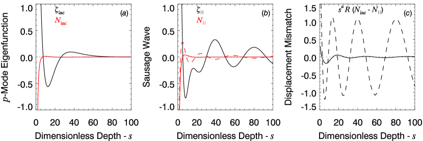
Figure 1: ($a$) The vertical displacement $\zeta_{\rm inc}$ (black curve) and the normal displacement to the flux tube’s surface $N_{\rm inc}$ (red curve) for an incident $p_{2}$ mode with a frequency of 3 mHz. ($b$) The vertical and normal displacements (black and red curves, respectively) for the sausage wave that is driven by the incident $p_{2}$ mode. The magnetic flux tube has a plasma parameter of $\beta=1$. ($c$) The resulting mismatch in the normal displacement between the $p$ mode and the sausage wave. In all panels the solid and dashed curves respectively represent the real and imaginary parts (when present).

Figure 1 illustrates the two displacement components for an incident $p_{2}$ mode, the components for the resulting sausage wave, and the mismatch between them $d_{n}$.

We can now solve for the two scattering matrices separately by invoking the orthogonality of the eigenfunctions and the jacket waves. In Appendix A we discuss that the weighting function for the orthogonality integrals is proportional to the mass density. If we make use of a dimensionless depth $s=-z/z_{0}$, the density within a neutrally stable atmosphere is a power law $\rho=\rho_{0}s^{a}$, where $\rho_{0}$ is the photospheric density and the polytropic index $a$ is related to the ratio of specific heats $\gamma$ through $a=(\gamma-1)^{-1}$. Multiply equation (3.7) by $s^{a}$ and the complex conjugate of either a $p$-mode eigenfunction $Q$ or a jacket wave $q$ and integrate over all depths to obtain,

$$S_{0}^{n\to n^{\prime}}(\omega) = \frac{i\pi}{2}\int_{1}^{\infty}ds\;s^{a}\;Q_{n^{\prime}}(\omega;s)\;d_{n}(\omega;s)\;,$$ (3.9)

$$T_{0}^{n\to\Lambda}(\omega) = \int_{1}^{\infty}ds\;s^{a}\;q^{*}(\omega,\Lambda;s)\ d_{n}(\omega;s)\;.$$ (3.10)

The limits of integration correspond to the photosphere ($s=1$) and infinitely deep into the solar interior.

Each element of the scattering matrices can therefore be thought of as the projection of the mismatch between the incident and scattered waves onto each $p$-mode and jacket-mode eigenfunction. The matrix associated with the far-field scattering, $S_{0}^{n\to n^{\prime}}(\omega)$ can be easily obtained by direct numerical integration of equation (3.9). We have used a Bulirsch-Stoer numerical integrator to perform these integrations and the results are discussed in the following sections. The integral that must be computed to obtain $T_{0}^{n\to\Lambda}(\omega)$ is fundamentally more difficult to numerically compute since jacket wavefunctions are not confined to an acoustic cavity and remain propagating to any depth. Therefore, while the magnitude of the integrand does vanish as $s\to\infty$, it does so slowly as a power law. This is unlike the integrand of Equation (3.9) which behaves like the product of a power law times a rapidly decaying exponential as $s\to\infty$. Therefore, we delay the calculation of the near-field scattering matrix to a subsequent time. Fortunately, the far-field and near-field scattering matrices are independent of each other due to the orthogonality of the $p$ modes and the jacket modes; thus, using this technique to calculate the far-field scattering matrix avoids the necessity of computing the acoustic jacket simultaneously.

Under many reasonable boundary conditions, one can demonstrate that the far-field scattering matrix $S_{0}^{n\to n^{\prime}}$ is symmetric under exchange of $n$ and $n^{\prime}$ (see Appendix D for a derivation). Here we apply a stress-free condition at the photosphere (for both the $p$ modes and the sausage waves) and finite energy (for the $p$ modes) and radiation (for the sausage waves) boundary conditions deep in the atmosphere (as $s\to\infty$). These boundary conditions are among those for which the scattering matrix is symmetric. This means that we need not calculate all of the matrix elements, only a little more than half need to be computed directly with the remaining obtained by symmetry.

4 Absorption and Mode Mixing

The absorption coefficient is often considered to be a measurement of energy loss or dissipation. When mode mixing occurs, this simple scenario needs to be modified as in addition to true absorption (or removal of energy from the acoustic wavefield), energy can be shuffled between modes by mode mixing. In this section we calculate the energy budget for a single incident wave and account for all the ways that the incident wave energy can be reprocessed by the scatterer. When the scatterer is an axisymmetric thin flux tube, there are only three ways in which energy can be extracted. (1) The single incident wave can excite tube waves which subsequently propagate out of the acoustic cavity. This mechanism is a true absorption process whereby acoustic energy is removed from the system. (2) The incident wave can generate an acoustic jacket that surrounds the flux tube. This mechanism is only significant for initial value problems and not for a spectral treatment as performed here. (3) The incident wave is scattered into outgoing waves of a different mode order. This last effect is mode mixing which is not true absorption as the acoustic energy remains in the cavity, albeit at a different wavenumber. We will assess the relative importance of the first and third mechanisms and leave the second to subsequent work.

4.1 Energy Budget of a Single Incident Wave

Consider a single incident wave of order $n$, with a unit amplitude (${\cal A}_{mn}=1$). This incident wave generates a set of outgoing waves with mode orders $n^{\prime}$. These outgoing waves can be written as follows, where we have included both the far-field scattered waves and the outgoing component of the incident wave,

$$\Phi_{\rm out}(\omega;r,z)=\sum_{n^{\prime}=0}^{\infty}\left[\frac{1}{2}\delta_{nn^{\prime}}+S_{0}^{n\to n^{\prime}}(\omega)\right]H_{m}^{(1)}(k_{n^{\prime}}r)\;Q_{n^{\prime}}(\omega;z)\;.$$ (4.1)

The term in square brackets is the amplitude of the outgoing wave of mode order $n^{\prime}$, and is composed of a contribution from the incident wave ($\delta_{nn^{\prime}}/2$) and from a scattered wave ($S_{0}^{n\to n^{\prime}}$). If the vertical eigenfunctions $Q_{n}$ are normalized according to equation (A6), each outgoing wave carries a lateral energy flux $F_{n^{\prime}}$ with the following form,

$$F_{n^{\prime}}=\frac{1}{2}\,\rho_{0}\,\omega^{3}z_{0}\left|\delta_{nn^{\prime}}+2S_{0}^{n\to n^{\prime}}\right|^{2}\;.$$ (4.2)

Note, the energy flux only depends on the mode order $n^{\prime}$ (and the azimuthal order $m$) through the amplitude. Therefore, the fraction $\varepsilon_{nn^{\prime}}$ of the ingoing wave’s energy that is re-emitted in mode order $n^{\prime}$ has similar dependence on the scattering matrix as exhibited by the absorption coefficient,

$$\varepsilon_{nn^{\prime}}=\left|\delta_{nn^{\prime}}+2S_{0}^{n\to n^{\prime}}\right|^{2}\;.$$ (4.3)

For this example with only a single incident mode order, the absorption coefficient is by definition 1 minus the diagonal elements of this fractional energy flux,

$$\alpha_{n}\equiv 1-\varepsilon_{nn} = 1-\left|1+2S_{0}^{n\to n}\right|^{2}$$

$$= -4{\rm Re}\left\{S_{0}^{n\to n}\right\}-4\left|S_{0}^{n\to n}\right|^{2}\;.$$

Of course this equation is identical to equation (2.10). By energy conservation, we can decompose this absorption coefficient into two parts, a true absorption from the excitation and escape of sausage waves $W_{n}$ and a redistribution term arising from mode mixing $M_{n}$,

$$\alpha_{n}=W_{n}+M_{n}.$$ (4.5)

The contribution from mode mixing $M_{n}$ can be directly written down using the off-diagonal elements of the fractional energy loss $\varepsilon_{nn^{\prime}}$,

$$M_{n}=\sum_{n^{\prime}\neq n}\varepsilon_{nn^{\prime}}=4\sum_{n^{\prime}\neq n}\left|S_{0}^{n\to n^{\prime}}\right|^{2}.$$ (4.6)

Therefore, by combining equations (4.1) and (4.6), the loss of energy due to the excitation of tube waves must have the following expression,

$$W_{n}=-4{\rm Re}\left\{S_{0}^{n\to n}\right\}-4\sum_{n^{\prime}=0}^{\infty}\left|S_{0}^{n\to n^{\prime}}\right|^{2}.$$ (4.7)

Before we can use any of these expressions, we need to consider the order of each of their terms. Since we have computed the scattering matrix to only leading order in the radius of the tube, ${\rm O}\left(R^{2}\right)$, for self-consistency we must drop the last term in equations (4.1) and (4.7),

$$\alpha_{n}(\omega)=-4{\rm Re}\left\{S_{0}^{n\to n}\right\}+{\rm O}(R^{4})\;,$$ (4.8)

$$W_{n}(\omega)=-4{\rm Re}\left\{S_{0}^{n\to n}\right\}+{\rm O}(R^{4})\;.$$ (4.9)

To lowest order, the absorption coefficient and the excitation rate of tube waves are identical. Therefore, our calculation of the absorption coefficient is only compatible with tube-wave generation. The terms due to mode mixing appear at higher orders which are not represented self-consistently. Fortunately, we can evaluate the mode mixing terms separately using the far-field scattering matrix through equations (4.3) and (4.6).

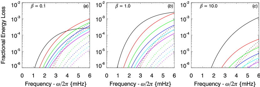
Figure 2: Fractional energy lost from the incident wave as a function of frequency for 100 km radius flux tubes with the three indicated values of the plasma parameter $\beta$. The colors indicate the order of the incident waves ($f$: black, $p_{1}$: red, $p_{2}$: green, $p_{3}$: blue, $p_{4}$: aqua, $p_{5}$: violet). The solid curves are the absorption coefficient $\alpha_{n}$ computed with the scattering matrix using equation (4.8). The dotted curves correspond to the energy lost from the incident mode order due to mode mixing into all other mode orders, $M_{n}$, equation (4.6). The energy loss arising from mode mixing is generally small compared to the tube wave excitation, although at high frequencies ($>5$ mHz) the mode mixing can climb to one-third of the total energy loss. Further, for the $f$ mode in the limit of large frequency, the absorption asymptotes to zero, leading to the property that the mode mixing can dominate the energy loss. The transition into this regime occurs when the wavelength of the sausage wave becomes much larger than the evanescence length of the $f$ mode; thus, the transition frequency increases as $\beta$ increases.

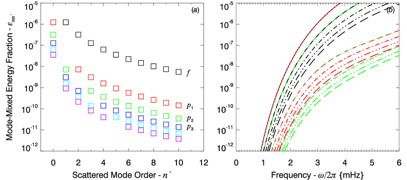
Figure 3: Fractional energy lost from the incident mode due to mode mixing induced by a magnetic tube with plasma parameter $\beta=1$ and a radius of 100 km. ($a$) Energy lost to each mode order of scattered waves for an incident wave of 3 mHz in frequency. The labels and the different colors correspond to the order of the incident wave, using the same color scheme as in Figure 2. ($b$) Energy lost to mode mixing as a function of frequency. The colors indicate the incident mode order ($f$ through $p_{2}$), while the linestyles correspond to different orders of the scattered modes ($f$: solid, $p_{1}$: dots, $p_{2}$: short dashes, $p_{3}$: dot-dashed, $p_{3}$: three dots and a dash, $p_{4}$: long dashes). In both panels careful examination verifies that the modulus of the scattering matrix is symmetric, $|S_{0}^{n\to n^{\prime}}|=|S_{0}^{n^{\prime}\to n}|$.

Figure 2 illustrates the absorption coefficient (solid curves) evaluated through the use of equation (4.8). The fraction of the incident energy, $M_{n}$, mixed into all other modes is represented with the dotted curves. In Figure 3, the energy $\varepsilon_{nn^{\prime}}$ that is scattered into each individual mode is shown. From this figure, one can see that the amount of energy lost to mode mixing decreases as the order of either the scattered mode $n^{\prime}$ or the incident mode $n$ increases. The symmetry of the scattering matrix leads to the symmetry of $\varepsilon_{nn^{\prime}}$, which is apparent in Figure 3$a$ as the equal height of pairs of symbols of different color and in Figure 3$b$ as the overlying of curves.

For low-frequencies, the mode-mixing losses are rather inconsequential compared to the sausage-wave losses. However, for higher frequencies the amount of energy lost to mode mixing can be a relative high fraction of the total energy loss, perhaps reaching as high as a third for some parameters. Furthermore, for the $f$ mode at high frequencies the excitation of sausage waves becomes anomolously inefficient and the mode-mixing terms can be the dominant source of energy loss. A more in depth discussion of tube wave excitation by the $f$ mode appears later in §6.1.

5 Phase Shifts and Phase Correlations

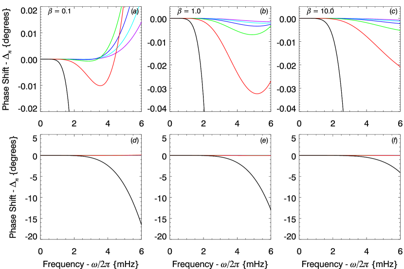
Figure 4: The phase shift as a function of frequency for flux tubes with a radius of 100 km and with the three indicated values of $\beta$. The different colors represent different incident mode orders ($f$: black, $p_{1}$: red, $p_{2}$: green, $p_{3}$: blue, $p_{4}$: aqua, $p_{5}$: violet). The bottom panels show the same quantity, but with a differently scaled ordinate in order to better illustrate the $f$ mode. Both positive and negative phase shifts are possible for $p$ modes and are universally small. Whereas for the $f$ mode, the shifts are negative and substantial, reaching values as large as -15^∘.

The computation of the scattering matrix also allows us to estimate phase shifts $\Delta_{n}$ through equation (2.12). These phase shifts are illustrated in Figure 4. For $p$ modes, both positive and negative phase shifts are possible, although all shifts become positive for sufficiently high frequency—which, depending on the value of $\beta$ may be beyond the physically relevant band of frequencies. The $f$ mode is fundamentally different. Not only is the phase shift for the $f$ mode negative for all frequencies, but the phase shift is large, reaching values as high as 15^∘ for high frequencies and for tubes with low values of the plasma parameter $\beta$.

The phases of all the scattered waves are correlated in a precise manner with the phase of the incident wave. The difference in phase $\Delta\phi_{nn^{\prime}}$ between each individual scattered wave and the incident wave can also be derived from the scattering matrix,

$$\Delta\phi_{nn^{\prime}}=\arg\left\{S_{0}^{n\to n^{\prime}}\right\}\;.$$ (5.1)

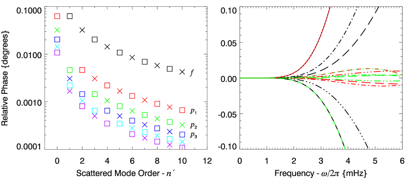
Figure 5: The phase of the scattered waves measured relative to the phase of the incident wave. ($a$) Absolute value of the phase of each mode order of scattered waves for an incident wave of 3 mHz in frequency. The $\times$ symbols correspond to positive phases and $\Box$ symbols to negative phases. The different colors (and labels) indicate the order of the incident wave. ($b$) Relative phase of each scattered wave as a function of frequency. The colors indicate the incident mode order ($f$ through $p_{2}$), while the linestyles correspond to different orders of the scattered modes as in Figure 3 ($f$: solid, $p_{1}$: dots, $p_{2}$: short dashes, $p_{3}$: dot-dashed, $p_{3}$: three dots and a dash, $p_{4}$: long dashes). In both panels careful examination verifies that the phase of the scattering matrix is symmetric, $\arg\{S_{0}^{n\to n^{\prime}}\}=\arg\{S_{0}^{n^{\prime}\to n}\}$.

These relative wave phases are uniformly small (see Figure 5). The difference is positive for $n+n^{\prime}$ even and negative for $n+n^{\prime}$ odd. The symmetry of the scattering matrix to exchange of $n$ and $n^{\prime}$ appears in Figure 5 as the overlying of curves and the equal height of symbols. In general, scattering to and from the $f$ mode results in larger phase differences, exceeding scattering between $p$ modes by an order of magnitude.

6 Discussion

We have calculated by semi-analytic means the scattering matrix for axisymmetric acoustic waves encountering a vertically-aligned, magnetic tube. We have assumed that the tube is slender and invoked the thin flux-tube approximation to compute the scattering matrix to leading order in the tube’s radius $R$ for mode orders up to $n=10$. In the following two sections we discuss the implications of the results of our calculation, both in terms of the energy budget of the incident and scattered waves and in terms of the phases of the outgoing waves.

6.1 Absorption and Energy

When encountering a thin flux tube of the type discussed here, a $p$ mode of a particular radial order $n$ may lose energy in either of two ways. The incident acoustic wave can excite MHD tube waves on the magnetic fibril that freely propagate along the tube carrying energy out of the acoustic cavity. This represents a true absorption as acoustic energy is removed from the wavefield. The tube may also scatter the incident $p$ mode into outgoing waves of different radial order $n^{\prime}$. Mode mixing of this sort does not represent a true absorption as the energy is merely redistributed between radial orders. Despite this fact, mode mixing can modify the observed absorption coefficient, as the definition of this coefficient does not take power redistribution into account. These two mechanisms are both inherently weak for thin tubes. The thin tube approximation mandates that the excitation of tube waves generates an absorption coefficient that scales linearly with the magnitude of the scattering matrix, which in turn scales like the square of the tube’s radius $R^{2}$, a small quantity by definition. The energy losses due to mode mixing are even smaller, scaling as the square of the magnitude of the scattering matrix, or as $R^{4}$. Therefore, mode mixing can only be important energetically when other sources of absorption (i.e., tube wave excitation) are peculiarly small. Over the physically relevant range of frequencies ($<6$ mHz), our calculations reveal that mode-mixing dominates the absorption coefficient only for high-frequency $f$ modes interacting with low-$\beta$ tubes.

Any model with a reflective upper boundary can have special frequencies for which the excitation of tube waves is unusually tiny. If the upper boundary reflects all wave energy, the excitation can formally be zero at these frequencies. Such “excitation nulls” arise because of total destructive interference. A localized driver, such as an incident $p$ mode, excites waves that propagate both up and down the tube with equal energy. At these special frequencies, the upward propagating wave reflects off the upper surface with just the phase needed to cancel the downward propagating wave (Jain et al., 2009; Crouch & Cally, 1999). In such a circumstance the downward energy flux vanishes and no energy is carried away from the acoustic cavity by tube waves. Near such an excitation null, the energy losses arising from mode mixing could be the dominant source of energy loss—not because mode mixing is large, but because the other source of absorption is small.

For the stress-free upper boundary condition applied here and for reasonable atmospheric and tube parameters, excitation nulls do not appear within the physically relevant frequency band ($\omega/2\pi<6$ mHz). However, formally for the $f$ mode such a null exists in the limit of infinite frequency and it has extremely broad influence, causing the absorption coefficient to asymptote to zero as the frequency becomes large. The frequency regime for which this asymptotic behavior is valid depends on $\beta$, with lower $\beta$ pushing the behavior to lower frequencies. Physically, such behavior exists because the $f$ mode is a surface wave that becomes increasingly confined to the photospheric layers as the frequency increases. The $f$ mode’s evanescence length $k^{-1}$ can be derived directly from its dispersion relation $\omega^{2}=gk$, revealing that the vertical extent of the $f$ mode scales as $\omega^{-2}$. The wavelength $L$ of the sausage wave at the photospheric surface can be derived from Equation (B12),

$$L=\left[\frac{(\gamma-1)g}{\left(1+\gamma\beta/2\right)z_{0}}\right]^{1/2}\frac{\pi}{\omega}\;.$$ (6.1)

As the frequency increases, $L$ shrinks, scaling as $\omega^{-1}$; however, it decreases more slowly than the scale length of the $f$ mode decreases (which scales as $\omega^{-2}$). Therefore, as the frequency increases, compared to the tube wave the driver looks more and more like a delta function located at the surface. A delta-function driver generates waves that propagate in each direction with identical amplitude and phase. If one of those components subsequently reflects off a surface and passes back through the driving layer, there is the potential for destructive interference (as discussed previously). Destructive interference occurs if the phase of the reflected wave advances by an odd integer factor of $\pi$. This phase advance can come from a phase change on reflection or from propagation of the wave to the reflecting layer and back. For the $f$ mode, one can show that the phase change on reflection asymptotes to $-\pi$ as the frequency becomes large (see Appendix C). Therefore, the $f$ mode, in the limit of infinite frequency, satisfies the necessary resonance condition because the distance between the driving layer and the photospheric reflection layer vanishes.

The $p$ modes do not evince such high-frequency behavior for the simple reason that at high frequency, the depth of the cavity becomes roughly constant with frequency. The wavenumber eigenvalue $k_{n}(\omega)$ scales linearly with the frequency, thereby causing the horizontal phase speed $\omega/k$ and the lower turning point of the $p$ mode to approach constants. Since, the depth of the cavity and hence the vertical extent of the driving region does not change as the frequency changes, the wavelength of the sausage waves becomes much shorter than that of the $p$ modes. Thus, for incident $p$ modes, the driving region remains vertically distributed and the arguments that we made previously for the $f$ mode are not valid.

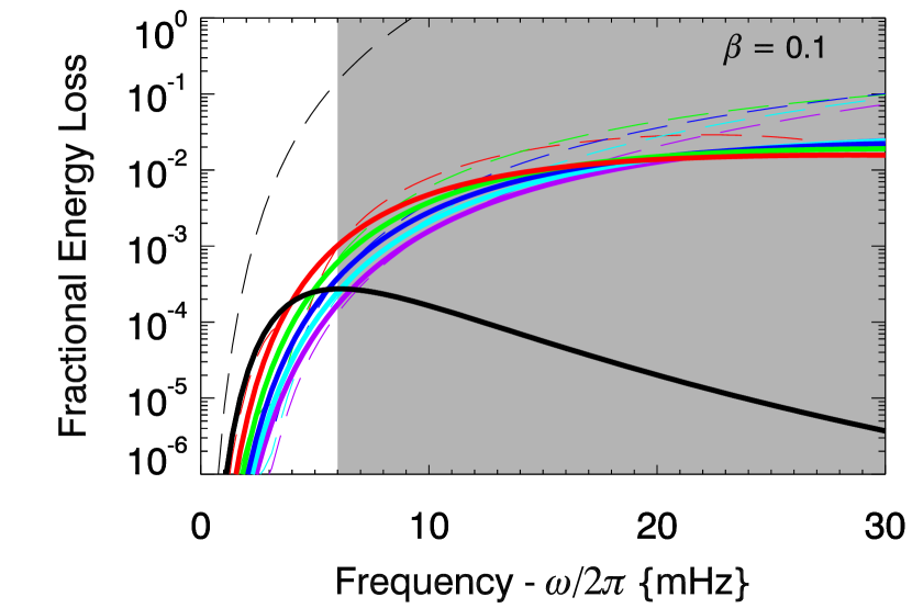
Figure 6: The high-frequency behavior of the absorption profiles. The thick solid curves are the absorption coefficient calculated via the far-field scattering matrix with equation (4.8), with the different colors indicating the order of the incident mode. The $f$ mode’s high-frequency behavior is fundamentally different from the $p$ modes because it is a surface wave. At high frequency, driving from the $f$ mode becomes spatially localized at the surface, wheras the driving from $p$ modes remains spatially distributed. The thin, dashed curves show the modulus of the scattering matrix $\left|S_{0}^{n\to n}(\omega)\right|$. For the perturbation scheme used here, the scattering matrix must be a small quantity. Clearly, for the $f$ mode, this weak-scattering approximation is invalid for frequencies exceeding roughly 6 mHz (the shaded region). We show such large frequencies merely to illustrate the mathematical behavior at high frequencies.

Figure 6 illustrates this behavior for $\beta=0.1$. While the figure extends to frequencies as large as 30 mHz, one must bear in mind that frequencies greater than 6 mHz are greater than the sun’s photospheric acoustic cutoff; thus, such waves are no longer trapped and the construction of our solar model is suspect. Further, one must be careful to not over-interpret the results at such extreme frequencies as the perturbation scheme has become invalid (see Figure 6). Despite this, for the $f$ mode, trapped waves of low frequency (where the perturbation analysis remains valid) can still sense the presence of the excitation null at infinity, causing a high-frequency fall-off of the absorption. The frequency of waves affected depends on the plasma parameter $\beta$ of the tube because the wavelength of the tube wave depends on $\beta$. We can estimate the lowest frequencies that should be affected by requiring that the wavelength of the sausage waves $L$ be two or three times larger than $f$ mode’s evanescence length $k^{-1}$. If we require that the ratio of these length scales satisies $kL>2$, we discern that for $\beta=0.1$ we would expect the high frequency regime to exist for frequencies above 3 mHz, whereas for $\beta=10$ the regime begins around 10 mHz.

This discussion only holds for absorption and mode mixing resulting from the excitation of the slow sausage wave. Similar calculations performed with fast kink oscillations reveal that excitation nulls can appear for all incident mode orders at frequencies less than 6 mHz (Jain et al., 2009; Crouch & Cally, 1999); also see Tirry (2000) for a similar phenomenon in an unstratified model. Further, the calculations of the scattering matrix elements arising from coupling to kink oscillations ($S_{\pm 1}^{n\to n^{\prime}}$) (Hanasoge et al., 2008) show significant oscillatory modulation in the magnitudes as a function of frequency, whereas our scattering calculation for the axisymmetric sausage wave ($S_{0}^{n\to n^{\prime}}$) show smooth frequency variation. In fact one could fit the magnitude of the scattering matrix calculated here with a single power law in frequency that would be roughly valid over all but the highest frequencies.

In a real plage, we do not expect such excitation nulls to have an easily identifiable effect other than a diminution of absorption at high frequencies for the $f$ mode. Not only does mode mixing tend to fill in the absorption profile, but the plage is likely to be comprised of a large number of tubes with a distribution of properties, including photospheric radius $R_{0}$ and plasma parameter $\beta$. Therefore, each tube in the collection will have suppressed absorption over a different range of frequencies. The added affect of all of the tubes will be to mitigate the effect of nulls (Jain et al., 2011). In general, we expect most flux tubes in a plage to have a near equipartition of magnetic and gas pressure, thus tubes with $\beta\approx 1.0$ should predominate. A quick examination of Figure 2 reveals that only the most extreme frequencies are likely to be affected.

To summarize, we find that for thin tubes, mode mixing is a small effect compared to tube wave excitation. The scattering matrix itself has elements that are proportional to the cross-sectional area of the tube. Tube wave excitation extracts energy at a rate proportional to the scattering matrix (or proportional to the cross-sectional area of the tube) while mode mixing redistributes energy at a rate proportional to the square of the scattering matrix.

6.2 Wave Phases

Phase shifts are generally defined as the difference in phase between the outgoing wave in the presence of the scatterer and the phase that would have existed in the absence of the scatterer. A magnetic tube can generate a phase shift by three distinct mechanisms: (1) The ingoing acoustic wave reflects off the lateral surface of the tube, shortening the total path length traveled by the wave. (In the absence of the tube, the wave would travel all the way to the coordinate axis and back.) Since the wave travels a shorter distance, the presence of the tube causes a phase lag resulting in a negative phase shift or travel-time difference. (2) The wave is at least partially transmitted through the lateral surface and propagates at a different speed within the magnetic tube. If the phase speed increases, a negative phase shift is achieved. (3) Upon reflection off the lateral surface of the tube, the wave can undergo a phase change. Off course if a flux-tube boundary could be treated as a rigid, impenetrable surface, the phase change would be 180 degrees. But, in general a flux tube is elastic and the phase change may differ from 180 degrees and may be either positive or negative.

For our thin flux-tube model, the only wave permitted within the tube is a sausage wave corresponding to a slow surface wave (see Roberts & Webb, 1978; Edwin & Roberts, 1983). For such a wave, the thin flux-tube approximation precludes lateral variation by implicitly assuming that the wave crossing time is much shorter than the wave period. Thus, for all tubes the crossing time for the tube should be ignored, resulting in a common negative phase shift, independent of $\beta$. Obviously the phase shift whould be equal to the phase lag that would have occured in the unmagnetized model for a wave propagating a distance equal to the tube diameter. This shows that for thin flux tubes, mechanisms 1 and 2 discussed in the previous paragraph are essentially the same. This is not true for thicker tubes for which the travel time across the tube is significant. A rough estimate of the expected phase shift would be $-2kR_{0}$, where $R_{0}$ is the photospheric radius of the tube and we have assumed that the phase lag should be evaluated at the photospheric surface. This is clearly appropriate for the $f$ mode as it is a surface wave confined to this layer. For $p$ modes one should probably consider a depth weighted average of the tube radius. However, for our purposes, the previous expression will suffice. Estimates made this way for the $f$ mode give a phase shift of $\Delta_{0}=-2\omega^{2}R_{0}/g$, which for waves at 3 mHz give a phase shift of -15^∘. This surprisingly large shift is about a factor of four larger than the phase shifts we obtain with our model (see 4), indicating that a phase change upon reflection is likely to be at work as well. We point out that despite the large size of the estimated shift, it is quite similar in magnitude and of the same sign as actually measured phase shifts for small magnetic features. Duvall et al. (2006) measured the average scattering from roughly 2500 small magnetic elements, and generated a typical travel time kernel from their measurements. One can obtain a typical phase shift of -14^∘ by the following process. Multiply the largest value of the measured kernel in Figure 6 from Duvall et al. (2006) (roughly -20 s kG^-1 Mm^-1) by the average magnetic flux of the studied features (0.6 kG Mm²) to obtain a travel time lag of -12 s. Convert this time lag into a phase shift by dividing by a wave period (300 s) and multiplying by 360 degrees.

The phase change that occurs at reflection from the lateral boundary of the flux tube is difficult to estimate, as the reflection depends on both the incident wave and the driven sausage wave over a range of heights. We would like to receive guidance from calculations performed for unstratified, thin tubes, for which analytic solutions are possible (e.g., Edwin & Roberts, 1983). However, the regime in frequency–wavenumber space for which slow surface waves exist and for which propagating external acoustic waves exist are disjoint. Thus, for unstratified tubes a propagating acoustic wave cannot excite slow surface waves. The stratification in our model is what makes the coupling possible. We can safely say, however, that the phase shift caused by mechanisms 1 and 2 always result in negative shifts for thin tubes. Further, we would expect the phase change upon reflection (mechanism 3) to increase for tubes of higher $\beta$ since such tubes are more elastic. For the $f$ mode this is indeed what we achieve; the phase shift is large and negative at all frequencies (probably as a result of a reduced path length) and becomes less negative as $\beta$ increases (probably due to an increasing positive phase change at reflection). However, for $p$ modes we obtain shifts of both signs; negative phase shifts at low frequency and positive shifts at high frequency. Clearly for the $p$ modes a positive phase change upon reflection at the flux-tube boundary must occur for at least high frequencies.

Appendix A The Field-Free Atmosphere and its Eigenfunctions

The field-free atmosphere that surrounds the magnetic flux tube is treated as a plane-parallel, neutrally stable polytrope. This atmosphere has been utilized extensively in the past as its a good representation of a stellar convection zone and simplifies the wavefield by imposing a condition of irrotationality. Gravity is uniform, acting in the downwards direction ${\mbox{{\boldmath$g$}}}=-g\hat{z}$, with the height coordinate $z$ increasing upward. The atmosphere is polytropic below the height $z=-z_{0}$, which corresponds to the model’s photosphere. The gas pressure, mass density and sound speed vary with height as power laws. If we employ a nondimensional depth $s=-z/z_{0}$, the background thermodynamic variables become,

$$P_{\rm ext} = \frac{gz_{0}\rho_{0}}{a+1}\;s^{a+1}=P_{0}\;s^{a+1}\;,$$

$$\rho_{\rm ext} = \rho_{0}\;s^{a}\;,$$

$$c_{\rm ext}^{2} = \frac{gz_{0}}{a}\;s\;.$$

The quantities $\rho_{0}$ and $P_{0}$ are the photospheric values of the mass density and gas pressure. The value of the polytropic index $a$ is set such that the stratification is neutrally stable to convection; this requires $a=1/(\gamma-1)$, where $\gamma$ is the ratio of specific heats. Above the photosphere $z=-z_{0}$, we assume the existence of a hot vacuum ($\rho_{\rm ext}\to 0$ with $T_{\rm ext}\to\infty$), with the property that the gas pressure ($P_{\rm ext}\sim\rho_{\rm ext}T_{\rm ext}$) is finite and continuous across the $z=-z_{0}$ layer.

Following Bogdan et al. (1996) and Hindman & Jain (2008), we specify the depth of the photosphere $z_{0}$ and the photospheric density $\rho_{0}$ (and therefore the reference pressure $P_{0}$) by matching our model photosphere to the $\tau_{5000}=1$ level of a solar model by Maltby et al. (1986). At this layer in the solar model $g=2.775\times 10^{4}$ cm s^-2, $\rho_{0}=2.78\times 10^{-7}$ g cm^-3, and $P_{0}=1.21\times 10^{5}$ g cm^-1 s^-2. We adopt a polytropic index of $a=1.5$, which is consistent with an adiabatic index of $\gamma=5/3$.

Since the buoyancy frequency in such an atmosphere is zero by definition, acoustic waves propagating within the atmosphere are irrotational. This permits such waves to be expressed using a displacement potential $\Phi$. If we assume oscillatory time dependence $~{}e^{-i\omega t}$ and harmonic functions with wavenumber $k$ in the horizontal direction, the vertical portion of the acoustic eigenfunction satisfies the following Sturm-Liouville equation,

$$\left[\frac{d}{ds}\left(s^{a}\frac{d}{ds}\right)+\nu^{2}s^{a-1}-\frac{\lambda^{2}}{4}s^{a}\right]Q(\nu;s) = 0\;,$$ (A1)

$$\lambda \equiv 2kz_{0}\;,$$ (A2)

$$\nu^{2} \equiv \frac{a\omega^{2}z_{0}}{g}\;,$$ (A3)

where $\lambda$ is a dimensionless horizontal wavenumber, $\nu$ is a dimensionless frequency and $Q$ represents either a discrete eigenfunction $Q_{n}(\nu;s)$ for real $\lambda=\lambda_{n}=2k_{n}z_{0}$ or a spectrum of jacket modes $q(\nu,\Lambda;s)$ for continuous, imaginary values of $\lambda=-2i\Lambda z_{0}$.

The general solutions to this equation are proportional to Whittaker $M$ and $W$ functions (Whittaker & Watson, 1952; Abramowitz & Stegun, 1964). The discrete $f$ and $p$ modes reside within an acoustic cavity and therefore become evanescent deep in the atmosphere. Thus, the $W$ functions are relevant as they decay exponentially as $s\to\infty$,

$$Q_{n}(\nu;s)=C_{n}(\nu)\;s^{-(\mu+1/2)}\;W_{\kappa_{n},\mu}(\lambda_{n}s)\;.$$ (A4)

Here $C_{n}(\nu)$ is a normalization constant and

$$\mu\equiv(a-1)/2\;,\qquad\kappa_{n}\equiv{\displaystyle\frac{\nu^{2}}{\lambda_{n}}}\;.$$

The quantization of the horizontal wavenumber $k_{n}$ (or equivalently $\lambda_{n}$) arises from the requirement that the Lagrangian pressure perturbation vanish at the model photosphere.

The laterally evanescent jacket waves are surface waves (with a lateral decay length of $\Lambda^{-1}$) that propagate up and down the outside of the flux tube. They are not trapped within the acoustic cavity and can freely propagate to any depth. If we select only those jacket waves that satisfy the condition that the Lagrangian pressure perturbation vanishes at the model photosphere, the jacket waves are standing waves that can be represented as a sum of Whittaker $M$ functions with imaginary argument (see Bogdan & Cally, 1995),

$$q(\nu,\Lambda;s)=C(\nu,\lambda)\;s^{-(\mu+1/2)}\;\left[\Gamma_{\kappa,\mu}(\lambda)\;M_{\kappa,\mu}(\lambda s)+M_{\kappa,-\mu}(\lambda s)\right]\;,$$ (A5)

where $C(\nu,\lambda)$ is a normalization constant and

$$\kappa\equiv\frac{\nu^{2}}{\lambda}\;,\qquad\Gamma_{\kappa,\mu}(\lambda)\equiv\frac{16(1+\mu)(1+2\mu)^{2}}{(1+2\mu)^{2}-\kappa^{2}}\frac{M_{\kappa,-(1+\mu)}(\lambda)}{M_{\kappa,1+\mu}(\lambda)}\;.$$

Unlike the $f$ and $p$ modes, for which the dimensionless horizontal wavenumber $\lambda$ is purely real and only takes on discrete values $\lambda_{n}$, for the jacket modes $\lambda$ is purely imaginary and continuous. Therefore, the argument and $\kappa$-index of the Whittaker functions in equation (A5) are purely imaginary as well.

Since both the discrete modes and the jacket modes satisfy Hermitian boundary conditions (vanishing Lagrangian pressure perturbation at both the photosphere $s=1$ and at infinity $s\to\infty$), we automatically know that the discrete, acoustic modes and the jacket modes are all mutually orthogonal with a weight function $s^{a}$ (which is proportional to the mass density),

$$\int_{1}^{\infty}ds\;s^{a}\;Q_{n}(\nu;s)\;Q_{n^{\prime}}(\nu;s) = \delta_{nn^{\prime}}\;,$$ (A6)

$$\int_{1}^{\infty}ds\;s^{a}\;Q_{n}(\nu;s)\;q(\nu,\Lambda;s) = 0\;,$$ (A7)

$$\int_{1}^{\infty}ds\;s^{a}\;q^{*}(\nu,\Lambda;s)\;q(\nu,\Lambda^{\prime};s) = \delta(\Lambda-\Lambda^{\prime})\;.$$ (A8)

In writing these last equations, we have chosen $C_{n}(\nu)$ and $C(\nu,\lambda)$ such that the discrete modes and jacket modes are orthonormal.

Appendix B Sausage Waves

We have assumed the magnetic fibril is untwisted, straight, axisymmetric, vertically aligned and thin. Thin flux tubes are unable to support internal lateral structure and hence the total pressure is uniform across the tube and continuous with its external value. If we further assume that the tube is the same temperature as its surroundings, the total pressure must have the same scale height inside and outside the tube and the plasma parameter $\beta$, defined as the ratio of the gas pressure to the magnetic pressure, is constant with height inside the tube. Since we only consider tubes below the photosphere (i.e., $z<-z_{0}$), we need not worry about the rapid flaring of the tubes into a magnetic canopy that occurs within the chromosphere.

We ignore lateral variation of the magnetic field strength, and describe the tube’s internal gas pressure $P(z)$, mass density $\rho(z)$, sound speed $c(z)$, and field strength $B(z)$ by their axial values. These four quantities as well as the tube’s radius $R(z)$ can be described uniquely by the total magnetic flux $\Theta$ contained by the tube and by the plasma $\beta$,

$$P = \frac{\beta}{\beta+1}P_{\rm ext}\;,$$ (B1)

$$\rho = \frac{\beta}{\beta+1}\rho_{\rm ext}\;,$$ (B2)

$$c = c_{\rm ext}\;,$$ (B3)

$$\frac{B^{2}}{8\pi} = \frac{1}{\beta+1}P_{\rm ext}\;,$$ (B4)

$$\pi R^{2} = {\displaystyle\frac{\Theta}{B}}=\left(\frac{\beta+1}{8\pi P_{\rm ext}}\right)^{1/2}\Theta\;.$$ (B5)

Observations indicate that typical field strengths for small photospheric flux tubes are between 1 and 2 kG within both quiet sun and plage (e.g., Lagg et al., 2010; Martínez Pillet et al., 1997). Such field strengths indicate rough equipartition between magnetic and gas pressure. For a flux tube with $\beta=1$ embedded in the polytropic atmosphere described in Appendix A, the magnetic field strength at the photosphere is $B_{0}=1.2$ kG. By inserting the external pressure $P_{\rm ext}$ into the expression for the cross-sectional area of the tube (B5), one obtains the explicit dependence of the tube radius on depth,

$$R(s)=R_{0}s^{-(a+1)/4}$$ (B6)

where $R_{0}=\left(\Theta/\pi B_{0}\right)^{1/2}$ is the photospheric radius of the tube. For all illustrations we will assume $R_{0}=100$ km, a fairly typical value for the size of magnetic elements within solar plage (Lagg et al., 2010).

Thin flux tubes support a longitudinal magnetoacoustic wave known as the sausage wave. Here, these oscillations are driven by the pressure perturbation imposed by external $f$- and $p$-mode oscillations (e.g., Roberts & Webb, 1978). Using the formulation of Hindman & Jain (2008), to lowest order in the radius of the flux tube, the vertical displacement $\zeta_{\parallel}$ within the tube can be described by the following equation,

$$\left\{\frac{\partial^{2}{\;\;}}{\partial{t}^{2}}-c_{T}^{2}\frac{\partial^{2}{\;\;}}{\partial{z}^{2}}+\frac{\gamma g}{2}\frac{c_{T}^{2}}{c^{2}}\frac{\partial{\;\;}}{\partial{z}}\right\}\zeta_{\parallel}=\frac{\rho_{\rm ext}}{\rho}\frac{c_{T}^{2}}{V_{\rm A}^{2}}\left.\frac{\partial^{3}\Phi_{\rm inc}}{\partial z\partial t^{2}}\right|_{r=0}\;,$$ (B7)

where $c_{T}$ is the cusp or tube speed which depends on both the sound speed $c$ and Alfvén speed $V_{\rm A}$ within the tube,

$$c_{T}^{2}=\frac{c^{2}V_{\rm A}^{2}}{c^{2}+V_{\rm A}^{2}}\;,\qquad V_{\rm A}^{2}=\frac{B^{2}}{4\pi\rho}\;.$$

The right-hand side of Equation (B7) is due to the forcing by the incident wave and is evaluated at the flux tube’s axis, $r=0$. This forcing arises from the enforcement of continuity of total pressure across the boundary of the flux tube. We are allowed to consider only the incident waves in this pressure balance because the far-field and near-field scattering amplitudes are smaller than the incident wave by a factor of $R^{2}\ln R$.

The forcing provided by each individual incident $p$ mode can be obtained by evaluating the expression for the incident wavefield, Equation (2.2), at $r=0$ and inserting the result into the sausage wave equation. After Fourier transforming in time $t$, one obtains

$$\left\{c_{T}^{2}\frac{\partial^{2}{\;\;}}{\partial{z}^{2}}-\frac{\gamma g}{2}\frac{c_{T}^{2}}{c^{2}}\frac{\partial{\;\;}}{\partial{z}}+\omega^{2}\right\}\zeta_{\parallel}=\frac{\rho_{\rm ext}}{\rho}\frac{c_{T}^{2}}{V_{\rm A}^{2}}\omega^{2}\sum_{n=0}^{\infty}\;{\cal A}_{n}(\omega)\frac{dQ_{n}(\omega;z)}{dz}\;.$$ (B8)

Note that only the $p$ modes with $m=0$ contribute to the forcing of the sausage waves. All other azimuthal components vanish in the limit $r\to 0$.

We adopt a non-dimensional form for this equation by the following substitutions,

$$s=-\frac{z}{z_{0}}\;,\qquad\epsilon=\frac{2+\gamma\beta}{2}\;,\qquad f_{n}(s)=-\frac{\gamma(\beta+1)}{2}\frac{\nu^{2}}{s}\frac{dQ_{n}(\nu;s)}{ds}\,$$

producing

$$\left(\frac{d^{2}}{ds^{2}}+\frac{\mu+1}{s}\frac{d}{ds}+\frac{\nu^{2}\epsilon}{s}\right)\zeta_{\parallel}(s)=\sum_{n=0}^{\infty}\frac{{\cal A}_{n}}{z_{0}}f_{n}(s)\;.$$ (B9)

The solution of this equation is expressed using a Green’s function,

$$\zeta_{\parallel}(s) = \sum_{n=0}^{\infty}\frac{{\cal A}_{n}}{z_{0}^{2}}\zeta_{\parallel,n}(s)\;,$$ (B10)

$$\zeta_{\parallel,n}(s) = -\frac{i\pi}{2}z_{0}\left\{\psi_{\parallel}(s)\left[\Omega_{n}+{\cal J}_{n}^{*}(s)\right]+\psi_{\parallel}^{*}(s)\left[{\cal I}_{n}-{\cal J}_{n}(s)\right]\right\}\;.$$ (B11)

In this equation, $\psi_{\parallel}(s)$ and $\psi_{\parallel}^{*}(s)$ are the two solutions to the homogeneous equation, ${\cal J}_{n}(s)$ and ${\cal I}_{n}$ are interaction integrals over the driver, and $\Omega_{n}$ is a parameter that specifies the complex amplitude of the wave that reflects from the upper surface and thus determines the boundary condition at the model photosphere (see Hindman & Jain, 2008, for details),

$$\psi_{\parallel}(s) = s^{-\mu/2}H_{\mu}^{(1)}(2\nu\sqrt{\epsilon s})\;,$$ (B12)

$${\cal J}_{n}(s) \equiv \int_{1}^{s}d\sigma\;\sigma^{\mu+1}\psi_{\parallel}(\sigma)f_{n}(\sigma)\;,$$ (B13)

$${\cal I}_{n}\equiv\lim_{s\to\infty}{\cal J}_{n}(s) = \int_{1}^{\infty}d\sigma\;\sigma^{\mu+1}\psi_{\parallel}(\sigma)f_{n}(\sigma)\;.$$ (B14)

If we apply a stress-free boundary condition on the sausage wave at the photosphere, the boundary condition parameter has the following form,

$$\Omega_{n} = i\frac{\gamma(\beta+1)}{\pi}\;\nu^{2}\;\frac{{\cal Q}_{n}}{\cal H}-\frac{{\cal H}^{*}}{\cal H}{\cal I}_{n}\;,$$ (B15)

$${\cal H} \equiv \nu\sqrt{\epsilon}H_{\mu+1}^{(1)}(2\nu\sqrt{\epsilon})+(\beta+1)(\mu+1)H_{\mu}^{(1)}(2\nu\sqrt{\epsilon})\;,$$ (B16)

$${\cal Q}_{n} \equiv \left.Q_{n}(\nu;s)\right|_{s=1}\;.$$ (B17)

Figure 1$a,b$ illustrates the resulting sausage wave as well as the driving $p$-mode eigenfunction when the incident wave is a $p_{2}$ wave.

We can derive an expression for the normal displacement inside the tube using the definition for the divergence of the displacement vector $\xi$ in cylindrical coordinates,

$$\nabla\cdot{\mbox{{\boldmath$\xi_{\parallel}$}}}=\frac{\partial h_{\parallel}}{\partial r}+\frac{h_{\parallel}}{r}+\frac{\partial\zeta_{\parallel}}{\partial z}\;,\\$$ (B18)

where $h_{\parallel}$ is the radial displacement. In this equation we have utilized the axisymmetry of the sausage mode. This can be combined with the Taylor series expansion of the radial displacement,

$$h_{\parallel}(\omega;r,z)=r\left.\frac{\partial h_{\parallel}(\omega;r,z)}{\partial r}\right|_{r=0}+\cdots,$$ (B19)

which we evaluate at $r=R(z)$ to obtain

$$h_{\parallel}(\omega;R,z)=\frac{R(z)}{2}\left(\nabla\cdot{\mbox{{\boldmath$\xi_{\parallel}$}}}-\frac{\partial\zeta_{\parallel}}{\partial z}\right)\;.$$ (B20)

If we now use Equation A9 from Bogdan et al. (1996), which is a statement about pressure equilibration of the tube with its external environment,

$$\nabla\cdot{\mbox{{\boldmath$\xi_{\parallel}$}}}=\frac{\beta}{2+\gamma\beta}\left(-\frac{\delta P_{\rm inc}}{P}+\frac{2}{\beta}\frac{\partial\zeta_{\parallel}}{\partial z}+\frac{g\rho_{\rm ext}}{P}\zeta_{\parallel}\right).$$ (B21)

and combine equations (3.2) and (B20), we obtain after some manipulation

$$N_{\parallel}(\nu;s)=\frac{R(s)}{4}\;\frac{\gamma\beta}{\epsilon z_{0}}\left[\frac{d\zeta_{\parallel}}{ds}+\frac{\mu}{s}\zeta_{\parallel}(s)-\frac{\beta+1}{\beta}\frac{\nu^{2}}{sz_{0}}\Phi_{\rm inc}(\nu;s)\right].$$ (B22)

This displacement can be decomposed into seperate components driven by each incident mode, by utilizing Equations (2.2) and (B10),

$$N_{\parallel}(\nu;s) = \sum_{n=0}^{\infty}\frac{{\cal A}_{n}}{z_{0}^{2}}\;N_{\parallel,n}(\nu;s),$$ (B23)

$$N_{\parallel,n}(\nu;s) = \frac{R(s)}{4}\;\frac{\gamma\beta}{\epsilon z_{0}}\left[\frac{d\zeta_{\parallel,n}}{ds}+\frac{\mu}{s}\zeta_{\parallel,n}(s)-\frac{\beta+1}{\beta}\frac{\nu^{2}}{s}z_{0}Q_{n}(\nu;s)\right].$$ (B24)

Appendix C High-Frequency Asymptotics for Incident $f$ Modes

The eigenfunction for the $f$ mode is simple enough that we can perform high-frequency asymptotics to derive approximate analytic solutions for the interaction integral ${\cal I}_{0}$ and all quantities derived from it. The $f$ mode eigenfrequency is always $\omega^{2}=gk$ independent of the details of the stratification. The associated eigenfunction is just an exponential that grows with height $Q_{0}(\omega;z)=\exp(kz)$. In our dimensionless variables, these relations take the form $\nu^{2}=a\lambda/2$ and $Q_{0}(\nu;s)=\exp(-\nu^{2}s/a)$. The $f$ mode’s evanescence length is given by $a/\nu^{2}$ and as the frequency becomes large, the evanescence length becomes tiny, scaling as $\sim\nu^{-2}$. The $f$ mode’s eigenfunction is, therefore, progressively more confined to the photospheric surface as the frequency becomes large. The tube wave on the other hand has a wavelength that diminishes much more slowly. From equation (B12) the wavelength of the sausage wave can be seen to scale as $\sim\nu^{-1}$. Thus, in the interaction integral ${\cal I}_{0}$ —see equation (B14), the integrand is only significant near the lower limit of integration (near the photosphere) and the sausage wave can be considered long wavelength.

C.1 The Interaction Integral

After inserting the $f$-mode eigenfunction and the homogeneous sausage wave solution—equation (B12)—into equation (B14), we obtain

$${\cal I}_{0} = \frac{\gamma(\beta+1)}{2a}\nu^{4}\int_{1}^{\infty}ds\;F(s)\,e^{-\nu^{2}s/a}\;,$$ (C1)

$$F(s) \equiv s^{\mu/2}H_{\mu}^{(1)}\left(2\nu\varepsilon^{1/2}s^{1/2}\right)\;.$$ (C2)

Since the exponential term in the integrand has significant magnitude only very close to the lower limit of integration and the sausage wave is long wavelength compared to the exponential scale length, we may expand the function $F(s)$ in a Taylor series about $s=1$,

$$F(s)=F(1)+F^{\prime}(1)(s-1)+\frac{F^{\prime\prime}(1)}{2}(s-1)^{2}+\cdots$$ (C3)

If we define

$$h_{\mu}\equiv H_{\mu}^{(1)}\left(2\nu\varepsilon^{1/2}\right)\;,$$ (C4)

and perform the necessary derivatives, the following expression is obtained,

$$F(s) = h_{\mu}+\left(\mu h_{\mu}-\nu\varepsilon^{1/2}h_{\mu+1}\right)(s-1)$$ (C5)

$$+\frac{1}{2}\left[\left(\frac{3}{2}\mu^{2}-\mu-\nu^{2}\varepsilon\right)h_{\mu}-(\mu-1)\nu\varepsilon^{1/2}h_{\mu+1}\right](s-1)^{2}+\cdots$$

After inserting this expansion into the integral appearing in equation (C1), each term in the expansion can be integrated separately by analytic means, producing the following expansion for the interaction integral,

$${\cal I}_{0}=\frac{\gamma(\beta+1)}{2}\nu^{2}e^{-\nu^{2}/a}\left[h_{\mu}+\frac{a}{\nu^{2}}\left(\mu h_{\mu}-\nu\varepsilon^{1/2}h_{\mu+1}\right)-\frac{a^{2}\varepsilon}{\nu^{2}}h_{\mu}+{\rm O}\left(\nu^{-7/2}\right)\right]\;.$$ (C6)

The order of the missing terms was deduced by noting that for large frequency the large-argument expansion of the Hankel function in equation (C4) is appropriate. Therefore, $h_{\mu}\sim\nu^{-1/2}$ and the leading order frequency dependence for ${\cal I}_{0}$ is ${\rm O}(\nu^{3/2}e^{-\nu^{2}/a})$. To lowest order, the interaction integral should decay rapidly as the frequency increases.

C.2 Amplitude of the Downward Propagating Sausage Wave

The complex amplitude of the wave that reflects from the photosphere is given by the boundary condition parameter $\Omega$. For the stress-free upper boundary with an $f$-mode incident wave, the boundary condition parameter $\Omega_{0}$ takes on the following form,

$$\Omega_{0}=i\frac{\gamma(\beta+1)}{\pi}\;\nu^{2}\frac{e^{-\nu^{2}/a}}{\cal H}-\frac{{\cal H}^{*}}{\cal H}{\cal I}_{0}\;.$$ (C7)

If we now combine equations (C6) and (C7) we find asymptotically,

$$\Omega_{0}=\frac{\gamma(\beta+1)}{2}\;\nu^{2}\frac{e^{-\nu^{2}/2}}{\cal H} \left[\frac{2i}{\pi}-\nu\varepsilon^{1/2}h_{\mu+1}^{*}h_{\mu}-(\mu+1)(\beta+1)h_{\mu}^{*}h_{\mu}\right.$$ (C8)

$$\qquad+a(\mu+1)(\beta+1)\nu^{-1}\varepsilon^{1/2}h_{\mu}^{*}h_{\mu+1}-a\mu\nu^{-1}\varepsilon^{1/2}h_{\mu+1}^{*}h_{\mu}$$

$$\qquad+a^{2}\nu^{-1}\varepsilon^{3/2}h_{\mu+1}^{*}h_{\mu}+{\rm O}\left(\nu^{-3}\right)\left.\frac{}{}\right]$$

From equation (B11) we can easily see that well below the driving layer, as $s\to\infty$, the amplitude of the downward propagating sausage wave becomes proportional to $\Omega_{0}+{\cal I}_{0}^{*}$. Oddly, if we add expression (C8) to the complex conjugate of equation (C6) and collect terms of like order, all of the terms cancel to the order calculated. Therefore, for an incident $f$ mode, in the limit of infinite frequency, the reflected wave and the directly generated wave undergo complete destructive interference and infinite frequency should be considered an “excitation null”.

In this limit, the driver is essentially a delta function located at the surface. Therefore, the phase difference between the reflected wave and the directly generated downward wave can only accrue from a phase change upon reflection off of the photosphere. For destructive interference, this phase change must be $\pm\pi$. The actual phase change turns out to be $\Delta\theta=-\pi$, and this can be verified asymptotically. The phase change can be expressed using the ratio of the complex amplitudes of the upward propagating wave and the reflected wave. These can be obtained by evaluating equation (B11) at $s=1$,

$$\Delta\theta=\arg\left\{\frac{{\cal I}_{0}h_{\mu}^{*}}{\Omega_{0}h_{\mu}}\right\}\;.$$ (C9)

Since the frequency is large, the Hankel functions represented by $h_{\mu}$ can be expressed using their large argument expansions,

$$\Delta\theta\approx\arg\left\{\frac{{\cal I}_{0}}{\Omega_{0}}e^{-4i\nu\varepsilon^{1/2}}e^{i(\mu+1/2)\pi}\right\}\;.$$ (C10)

If we now compute the ratio ${\cal I}_{0}/\Omega_{0}$ using these same large argument expansions we find,

$$\frac{{\cal I}_{0}}{\Omega_{0}}=e^{4i\nu\varepsilon^{1/2}}e^{-i(\mu+3/2)\pi}\;.$$ (C11)

Combine these last two expressions to find that $\Delta\theta=-\pi$ to leading order.

Appendix D Symmetry of the Far-Field Scattering Matrix

In this appendix we will demonstrate that under several commonly used boundary conditions the far-field scattering matrix, $S_{0}^{n\to n^{\prime}}$, is symmetric to interchange of $n$ and $n^{\prime}$ $(S_{0}^{n\to n^{\prime}}=S_{0}^{n^{\prime}\to n})$. We start with equation (3.9),

$$S_{0}^{n\to n^{\prime}}=\frac{i\pi}{2}\int_{1}^{\infty}ds\;s^{a}Q_{n^{\prime}}(s)\,d_{n}(s)$$ (D1)

where the frequency dependence has been suppressed. First we need an expression for the mismatch, $d_{n}$, which is supplied by equation (3.7),

$$d_{n}(s)=\frac{R(s)}{z_{0}^{2}}\left[N_{{\rm inc},n}(s)-N_{\parallel,n}(s)\right]\;.$$ (D2)

Using equations (3.3), (B6) and (B24) this expression can be reduced to a sum of two terms: a term that depends solely on the incident $p$-mode eigenfunction and a term that depends on the excited sausage waves,

$$d_{n}(s)=\frac{R_{0}^{2}}{2z_{0}^{2}}\,s^{-a}\left\{s^{\mu}\left[\frac{\mu+1}{s}\frac{dQ_{n}}{ds}-\frac{\lambda_{n}^{2}}{4}Q_{n}(s)+\frac{\gamma(\beta+1)}{2\varepsilon}\frac{\nu^{2}}{s}Q_{n}(s)\right]-\frac{\gamma\beta}{2\varepsilon z_{0}}\frac{d}{ds}\left(s^{\mu}\zeta_{\parallel,n}\right)\right\}\;.$$ (D3)

The terms in the square brackets can be modified using the Sturm-Liouville differential equation that the $p$-mode eigenfunctions satisfy, equation (A1),

$$d_{n}(s)=-\frac{R_{0}^{2}}{2z_{0}^{2}}\,s^{-a}\left[\frac{d}{ds}\left(s^{\mu}\frac{dQ_{n}}{ds}\right)-\frac{(\gamma-2)}{2\varepsilon}\nu^{2}s^{\mu-1}Q_{n}(s)+\frac{\gamma\beta}{2\varepsilon z_{0}}\frac{d}{ds}\left(s^{\mu}\zeta_{\parallel,n}\right)\right]\;.$$ (D4)

Insert this expression into equation (D1) to obtain,

$$S_{0}^{n\to n^{\prime}}=-\frac{i\pi}{4}\frac{R_{0}^{2}}{z_{0}^{2}}\left\{{\rm D}_{n^{\prime}n}+\frac{\gamma\beta}{2\varepsilon z_{0}}\int_{1}^{\infty}ds\;Q_{n^{\prime}}(s)\frac{d}{ds}\left[s^{\mu}\zeta_{\parallel,n}(s)\right]\right\}\;,$$ (D5)

where the values ${\rm D}_{n^{\prime}n}$ are the elements of a differential operator, ${\bf D}$,

$${\bf D}\,Q(s) \equiv \frac{d}{ds}\left[s^{\mu}Q(s)\right]-\frac{\gamma-2}{2\varepsilon}\nu^{2}s^{\mu-1}Q(s)\;,$$ (D6)

$${\rm D}_{n^{\prime}n} \equiv \int_{1}^{\infty}ds\;Q_{n^{\prime}}(s){\cal\bf D}\,Q_{n}(s)\;.$$ (D7)

Since we have applied Hermitian boundary conditions to the $p$ modes, one can easily verify that the operator ${\bf D}$ is also Hermitian with respect to the same set of functions; thus, ${\rm D}_{n^{\prime}n}={\rm D}_{nn^{\prime}}$. So, we now only need consider the second term in the braces in equation (D5): Is this term symmetric upon exchange of $n$ and $n^{\prime}$?

The longitudinal displacement $\zeta_{\parallel,n}$ can easily be expressed using a Green’s function, $G(s,s^{\prime})$,

$$\frac{\zeta_{\parallel,n}(s)}{z_{0}}=-\frac{i\pi}{2}\Omega_{n}\psi_{\parallel}(s)+\int_{1}^{\infty}ds^{\prime}\;G(s,s^{\prime})f_{n}(s^{\prime})\;,$$ (D8)

where

$$G(s,s^{\prime}) = -\frac{i\pi}{2}s^{\prime(\mu+1)}\Psi(s,s^{\prime})\;,$$ (D9)

$$\Psi(s,s^{\prime}) \equiv \left\{{\psi_{\parallel}(s)\,\psi_{\parallel}^{*}(s^{\prime})\qquad{\rm if}\;s^{\prime}<s,\atop\psi_{\parallel}^{*}(s)\,\psi_{\parallel}(s^{\prime})\qquad{\rm if}\;s^{\prime}>s,}\right.$$ (D10)

$$f_{n}(s) = -\frac{\gamma(\beta+1)}{2}\frac{\nu^{2}}{s}\frac{dQ_{n}}{ds}\;.$$ (D11)

This formulation is different from the one used in Appendix B because we will exploit symmetries possessed by the Green’s function and the present formulation makes those symmetries explicit. In particular, note that the function $\Psi(s,s^{\prime})$ is symmetric upon the interchange of $s$ and $s^{\prime}$.

In expression (D8), $\Omega_{n}$ is a complex constant that determines the boundary condition applied to the sausage wave at the surface of the truncated polytrope. For a stress-free surface the appropriate value of $\Omega_{n}$ is given by,

$$\Omega_{n}=i\frac{\gamma(\beta+1)}{\pi}\nu^{2}\frac{{\cal Q}_{n}}{\cal H}-\frac{{\cal H}^{*}}{\cal H}{\cal I}_{n}\;,$$ (D12)

and, alternatively, for an upper atmosphere with minimal reflectivity (Hindman & Jain, 2008) the correct value of the boundary condition parameter $\Omega_{n}$ is

$$\Omega_{n}=-\frac{\gamma(\beta+1)}{2}\nu^{2}h_{\mu}{\cal Q}_{n}\;.$$ (D13)

If one inserts equation (D8) into expression (D5), integrates by parts, and uses the fact that the $p$-mode eigenfunctions and the tube wave solutions vanish at infinity ($s\to\infty$), one can obtain the following expression after some manipulation,

$$S_{0}^{n\to n^{\prime}}=-\frac{i\pi}{4}\frac{R_{0}^{2}}{z_{0}^{2}}{\rm D}_{n^{\prime}n}+\frac{\pi^{2}\gamma\beta}{16\varepsilon z_{0}}\frac{R_{0}^{2}}{z_{0}^{2}}\left(W_{n^{\prime}n}+B_{n^{\prime}n}\right)\;,$$ (D14)

where

$$W_{n^{\prime}n} \equiv \frac{\gamma(\beta+1)}{2}\nu^{2}\int_{1}^{\infty}\int_{1}^{\infty}ds\,ds^{\prime}\;s^{\mu}s^{\prime\mu}\Psi(s,s^{\prime})\frac{dQ_{n}^{\prime}}{ds}\frac{dQ_{n}}{ds^{\prime}}\;,$$ (D15)

$$B_{n^{\prime}n} \equiv \frac{\Omega_{n}{\cal I}_{n^{\prime}}}{\gamma(\beta+1)\nu^{2}}-{\cal Q}_{n^{\prime}}\left(h_{\mu}\Omega_{n}+h_{\mu}^{*}{\cal I}_{n}\right)\;.$$ (D16)

It is trivial to demonstrate that $W_{n^{\prime}n}$ is symmetric. Since the variables $s$ and $s^{\prime}$ in the integrals are dummy variables, we can exchange them ($s\to s^{\prime}$ and $s^{\prime}\to s$) and then exchange the order of integration. Further, the function $\Psi(s,s^{\prime})$ is symmetric to interchange of its two arguments. Therefore, after performing these exchanges we find the forestated symmetry, $W_{n^{\prime}n}=W_{nn^{\prime}}$.

Thus, the symmetry of the far-field scattering matrix hinges on the properties of the matrix $B_{n^{\prime}n}$, which contains boundary terms arising from the integration by parts as well as a contribution that comes from the homogeneous solution appearing in the first term in equation (D8). Under some common boundary conditions for the sausage waves, this matrix is symmetric, but in general it is not. One can readily verify by directly inserting expressions (D12) or (D13) into equation (D16), and using the identity for the Wronskian of two Hankel functions,

$${\cal W}\left\{H_{m}^{(1)}(x),H_{m}^{(2)}(x)\right\}=H_{m+1}^{(1)}(x)H_{m}^{(2)}(x)-H_{m}^{(1)}(x)H_{m+1}^{(2)}(x)=-\frac{4i}{\pi x}\;,$$ (D17)

that both of the boundary conditions mentioned previously (stress free and minimum reflectivity) produce a symmetric matrix, $B_{n^{\prime}n}=B_{nn^{\prime}}$. Therefore, at least for these two boundary conditions, the far-field scattering matrix is also symmetric.

The crucial properties that were required for this symmetry are (1) the $p$ modes satisfy Hermitian boundary conditions, (2) the sausage wave vanishes deep in the atmosphere ($s\to\infty$), and (3) the sausage wave satisfies a boundary condition at the surface of the truncated polytrope ($s=1$) that causes the boundary term matrix $B_{n^{\prime}n}$ to be symmetric (note, not necessarily vanishing). This proof is very reminiscent of the calculation that is performed to demonstrate that a differential operator is Hermitian; however, in this case the operator in question is actually an integro-differential operator (because of the integration over the Green’s function).

References

- Abramowitz & Stegun (1964) Abramowitz, M., & Stegun, I. A. 1964, Handbook of Mathematical Functions, (New York: Dover Publications), 507
- Andries & Cally (2011) Andries, J., & Cally, P.S. 2011, ApJ, in press
- Bogdan & Zweibel (1987) Bogdan, T. J. & Zweibel, E. G. 1987, ApJ, 312, 444
- Bogdan & Fox (1991) Bogdan, T. J. & Fox, D. C. 1991, ApJ, 379, 758
- Bogdan & Cally (1995) Bogdan, T. J. & Cally, P. S. 1995, ApJ, 453, 919
- Bogdan et al. (1996) Bogdan, T. J., Hindman, B. W., Cally, P. S., & Charbonneau, P. 1996, ApJ, 465, 406
- Braun (1995) Braun, D. C. 1995, ApJ, 451, 859
- Braun & Birch (2008) Braun, D. C., & Birch, A. C. 2008, Sol. Phys., 251, 267
- Cally & Bogdan (1993) Cally, P. S., & Bogdan, T. J. 1993, ApJ, 402, 732
- Cally (2000) Cally, P. S. 2000, Sol. Phys., 192, 395
- Cally et al. (2003) Cally, P. S., Crouch, A. D., & Braun, D. C. 2003, MNRAS, 346, 381
- Crouch & Cally (1999) Crouch, A. D., & Cally, P. S. 1999, ApJ, 521, 878
- Crouch & Cally (2003) Crouch, A. D., & Cally, P. S. 2003, Sol. Phys., 214, 201
- Defouw (1976) Defouw, R. J. 1976, ApJ, 209, 266
- D’Silva (1994) D’Silva, S. 1994, ApJ, 435, 881
- Duvall et al. (2006) Duvall, T. L., Jr., Birch, A. C., & Gizon, L. 2006, ApJ, 646, 553
- Edwin & Roberts (1983) Edwin, P. M., & Roberts, B. 1983, Sol. Phys., 88, 179
- Gordovskyy et al. (2009) Gordovskyy, M., Jain, R., & Hindman B. .W. 2009, ApJ, 694, 1602
- Haber et al. (1999) Haber, D., Jain, R. & Zweibel, E. G. 1999, ApJ, 515, 832
- Hanasoge et al. (2008) Hanasoge, S. M., Birch, A. C., Bogdan, T. J. & Gizon, L. 2008, ApJ, 680, 774
- Hanasoge & Cally (2009) Hanasoge, S. M. & Cally, P. S. 2009, ApJ, 697, 651
- Hindman & Jain (2008) Hindman, B. W. & Jain, R. 2008, ApJ, 677, 769 (HJ2008)
- Hollweg (1988) Hollweg, J. V. 1988, ApJ, 335, 1005
- Jain et al. (2009) Jain, R., Hindman, B. W., Braun, D. C. & Birch, A. C. 2009, ApJ, 695, 325
- Jain et al. (2011) Jain, R., Gascoyne, A., & Hindman, B. W. 2011, MNRAS, 415, 1276
- Keppens et al. (1994) Keppens, R., Bogdan, T. J., & Goossens, M. 1994, ApJ, 436 372
- Lagg et al. (2010) Lagg, A., Solanki, S. K., Riethmüller, T. L., Martínez Pillet, V., Schüssler, M., Hirzberger, J., Feller, A., Borrero, J. M., Schmidt, W., del Toro Iniesta, J. C., Bonet, J. A., Barthol, P., Berkfield, T., Domingo, V., Gandorfer, A., Knölker, M., & Title, A. M. 2010, ApJ, 723, L164
- Lou (1990) Lou, Y. Q. 1990, ApJ, 350, 452
- Maltby et al. (1986) Maltby, P., Avrett, E. H., Carlsson, M., Kjelsdeth-Moe, O., Kurucz, R. L., & Loeser, R. 1986, ApJ, 306, 284
- Martínez Pillet et al. (1997) Martínez Pillet, V., Lites, B. W., & Skumanich, A. 1997, ApJ, 474, 810
- Roberts & Webb (1978) Roberts, B., & Webb, A. R. 1978, Sol. Phys., 56, 5
- Spruit & Zweibel (1979) Spruit, H. C., & Zweibel, E.G. 1979, Sol. Phys., 62, 15
- Spruit (1982) Spruit, H. C. 1982, Sol. Phys., 75, 3
- Tirry (2000) Tirry, W. J. 2000, ApJ, 528, 493
- Whittaker & Watson (1952) Whittaker, E. T., & Watson, G. N. 1952, A Course of Modern Analysis, (Cambridge: Cambridge Univ. Press), chap. 16