Outflow dynamics of dust-driven wind models and implications for cool envelopes of PNe

Abstract

The density profiles of cool envelopes of young Planetary Nebulae (PNe) are reminiscent of the final AGB outflow history of the central star, so far as these have not yet been transformed by the hot wind and radiation of the central star. Obviously, the evolution of the mass loss rate of that dust-driven, cool wind of the former giant in its final AGB stages must have shaped these envelopes to some extent. Less clear is the impact of changes in the outflow velocity. Certainly, larger and fast changes would lead to significant complications in the reconstruction of the mass-loss history from a cool envelope’s density profile.

Here, we analyse the outflow velocity $v_{\rm exp}$ in a consistent set of over 50 carbon-rich, dust-driven and well “saturated” wind models, and how it depends on basic stellar parameters. We find a relation of the kind of $v_{\rm exp}\propto(L/M)^{0.6}$. By contrast to the vast changes of the mass-loss rate in the final outflow phase, this relation suggest only very modest variations in the wind velocity, even during a thermal pulse. Hence, we conclude that the density profiles of cool envelopes around young PNe should indeed compare relatively well with their recent mass-loss history, when diluted plainly by the equation of continuity.

1 Introduction

The intriguing detail displayed by PNe in visual wavelengths is the result of complex and dynamic interaction of very different phases of circumstellar matter, following rapid changes in stellar evolution. The ionizing UV radiation and hot, fast wind of the hot central star modifies a cool outer envelope from inside–out (Schönberner et al., 2005). In fact, many circular and elliptical PNe often show a double-shell structure which consists of a rim – seen as a bright inner ring – and the surrounding shell (Phillips et al., 2009, and references therein). The latter is material already heated up by the ionizing radiation. The inner rim, on the other hand, which appears to move with a velocity of $\sim$40 km s^-1, is caused by the interaction of the hot, fast wind of the central star with the cool, slowly expanding shell. The latter is the product of a recently ceased, cool, slow ($\sim$15 km s^-1), and dense dust-driven outflow, which accompanied the final asymptotic giant branch (AGB) stages of the star.

Renzini once coined the nickname “superwind” (Renzini, 1981) for this final, massive and dust-rich AGB mass loss. It is a result of the very efficient interaction of the stellar radiation of a cool AGB giant and the newly formed dust particles in its atmosphere. This superwind removes of the order of one solar mass in the course of about 30 000 years from the stellar envelope, prior to the very end of the AGB phase. This concerns stars with low- and intermediate initial mass, of about ($\sim$1–8 $M_{\odot}$), and their mass-loss rates can reach from $10^{-5}\,M_{\sun}$ yr^-1 to $10^{-4}\,M_{\sun}$ yr^-1.

A physical record of such a cool outflow can be found outside the visible structures of a young PN. By contrast to its spectacular optical counterpart, the cool envelope is not at all so easy to observe. Only the remarkable advances of observational means in the past two decades in the infrared (ISO satellite in the 90ies and Spitzer in the past decade) and millimeter-waves (IRAM, large advances in detector technology, leading to a promising potential of upcoming ALMA, see e.g. (Cox, 2001) have put such cool envelopes now in reach of human scrutiny.

Still, details of that outflow phase, and how it gives way to the observed variety of PNe – like circular, elliptical, or bipolar – are not yet fully understood. It seems clear only that the transition occurs when the stars are developing from the AGB to PNe, i.e. when they are in the short proto-planetary nebula phase (Fong et al., 2006). Unfortunately, this phase is rare to observe as it is short-lived (of the order of $10^{3}$ years). But the younger a PN is, the less has the evidence of its recent past – imprinted in its cool outer envelope – been modified by the hot central star.

In addition to all these questions of PN-formation, there is a further motivation to fully and quantitatively understand the final phase of mass loss on the AGB: The mass lost during this time determines, by a large proportion, how much mass actually remains in the stellar remnant, the white dwarf. In other words, work on superwinds also aims to reproduce the observed initial-final mass relation (Weidemann, 2000).

For a quantitative understanding of the radial density profile of a young PN’s cool, outer envelope, the mass-loss history is clearly not the only factor of importance. Equally well we should know, how fast the outflow was and how much its velocity was varying. Nevertheless, some cool PN envelopes appear to be reproduced quite well by means of a proper mass-loss history alone, by making the simplification that on the star’s evolutionary time-scale the outflow velocity did neither change too much nor too fast. This approach was taken by Phillips et al. (2009), who compared observed density profiles of PNe derived from Spitzer images to theoretical predictions of stellar evolution calculations which included a parameter-dependent mass-loss rate. The latter is based on models for a C-rich, dust-driven, and dense wind. Despite its simplicity, the assumption of constant outflow velocity still leads to reasonable agreement between models and observations. Hence, here we attempt a more detailed investigation of how much the outflow velocity is actually changing in the dense, C-rich, and dusty envelope of a red giant, close to the very end of its AGB stage.

There are, of course, immense limitations to the observational evidence of such objects. Hence, Habing et al. (1994) attempted such an investigation of outflow velocities based on theoretical arguments. For high mass-loss rates, $\dot{M}>10^{-5}\,M_{\sun}$yr^-1, they found a very modest dependence on stellar quantities: $v_{\text{out}}\propto L_{\star}^{0.3}\delta^{0.5}(\dot{M}/a)^{0.04}$, where $L_{\star}$ is the stellar luminosity, $\delta$ the dust-to-gas ratio, and $a$ the grain size. The latter appears to have a nearly negligible influence on the outflow velocity. The same study found, observational evidence would match well such a small dependence of the outflow velocity on stellar parameters, i.e. on the luminosity.

We here want to take a new and different look at this problem by using the behaviour of the underlying hydrodynamical wind models – the same, which were used for the mass-loss parameterisation in Phillips et al. (2009) – with respect to the outflow velocity. We are checking the assumption of constant outflow velocity in our models by checking the average velocities of the dust-driven wind models against dependence on the basic stellar quantities.

2 Description of the wind models

For this investigation we use a set of hydrodynamical wind models that include formation and growth of dust grains which, by radiation pressure, drive massive outflows. These are characteristic of the ultimate stages of stellar evolution on the AGB.

The wind models have been obtained with the computer code developed by Fleischer et al. (1992), Winters et al. (2000), and references therein. They result from the selfconsistent solution of the non-linearly coupled system of equations describing the hydrodynamical and thermodynamical structure of a spherically symmetric stellar atmosphere (with a pulsating photosphere as an inner boundary condition, providing an initial mechanical energy input), its chemical composition, as well as the nucleation, growth, and evaporation of dust grains, and the radiation of the central star.

The hydrodynamical wind structure (mass density $\rho$ and outflow velocity $v$) follows from the equation of continuity and the equation of motion which includes the radiation pressure on dust grains. The law of energy conservation and radiative transfer determine the temperature structure.

A carbon-rich chemistry is assumed, where oxygen is completely locked in the CO molecule. The molecular composition is calculated under the assumption of chemical equilibrium. The formation, growth, and evaporation of carbon grains is calculated according to the moment method developed by Gail & Sedlmayr (1988) and Gauger et al. (1990). Schirrmacher et al. (2003) give a more detailed summary of the physical assumptions.

From a set of these models we derived a mass-loss formula for stars with solar element abundances, which have reached the tip of the AGB (Wachter et al., 2002). For that set of wind models, the velocity amplitude of the piston, used to simulate stellar pulsation, was set to a value of 5 km s^-1. That value was found to be in accordance with a sample of observed C-star lightcurves. The dependence of the mass-loss rates on the pulsation period was implicitly accounted for by the use of an observationally determined period-luminosity relation for Mira stars, the most appropriate class of objects on the tip of the AGB to compare with the hydrodynamical models. In this way we were able to represent the mass-loss rate by a simple relation dependent on the stellar parameters mass $M$, luminosity $L$, and effective temperature $T_{\rm eff}$, only. In this work, we follow a similar strategy in oder to find such a simple relation to represent the average wind velocity.

Table 1: Set of Berlin wind models used in this investigations. The piston velocity amplitude is fixed to $\Delta v$ = 5 km s^-1, see text for details.

$M$	$T_{\mathrm{eff}}$	$L$	C/O	$P$	$\langle\dot{M}\rangle$	$\langle v_{\text{exp}}\rangle$
[$M_{\odot}$]	[K]	[$L_{\odot}$]	[1]	[d]	[$M_{\odot}$/yr]	[km/s]
1.00	2600	10000	1.80	650	2.6E-05	31.8
0.80	3000	15000	1.50	650	3.0E-05	26.1
0.80	3000	15000	1.50	800	4.1E-05	25.4
0.80	3000	15000	1.50	300	1.7E-05	25.0
0.80	3000	7500	1.80	650	1.0E-05	34.2
0.80	3000	7500	1.80	450	8.3E-06	31.6
0.80	2200	15000	1.30	300	1.1E-04	16.6
0.80	2600	5000	1.30	400	1.3E-05	9.1
0.80	2600	4000	1.30	400	6.5E-06	6.5
0.80	3000	6000	1.30	400	3.8E-06	10.2
0.80	2600	7500	1.30	450	2.5E-05	11.3
0.80	2600	5000	1.30	300	7.4E-06	8.6
0.80	2500	6000	1.30	400	1.6E-05	10.0
0.80	2800	5000	1.30	400	6.1E-06	9.1
1.20	2600	7000	1.30	400	6.1E-06	7.9
0.80	2600	7000	1.30	450	1.9E-05	10.8
0.80	2600	12000	1.30	800	7.0E-05	16.2
0.80	2600	15000	1.30	1000	9.9E-05	16.6
0.80	2600	10000	1.30	640	5.0E-05	12.8
1.00	2600	10000	1.30	640	4.3E-05	12.6
1.00	2800	10000	1.30	640	1.8E-05	12.9
1.00	2900	10000	1.30	578	1.3E-05	13.1
1.00	2900	10000	1.25	578	9.6E-06	10.5
1.00	2900	10000	1.25	578	9.6E-06	10.5
1.00	2800	7000	1.30	400	5.4E-06	9.7
1.00	2800	8000	1.30	400	5.1E-06	12.0
1.20	2800	10000	1.50	400	1.6E-05	20.6
1.20	2800	10000	1.80	400	1.3E-05	30.9
0.80	2600	5000	1.30	350	6.4E-06	8.4
0.80	2600	5000	1.30	500	1.3E-05	9.3
0.80	2600	5000	1.30	600	1.6E-05	9.6
0.80	2600	7500	1.30	300	1.0E-05	11.8
0.80	2600	7500	1.30	600	5.1E-05	11.8
1.00	2400	12000	1.30	600	7.7E-05	14.7
1.00	2400	12000	1.30	300	2.6E-05	13.6
0.80	3000	7500	1.50	400	9.0E-06	21.6
0.80	2400	7500	1.50	104	1.4E-05	21.4
1.20	2800	10000	1.40	400	9.8E-06	16.9
0.80	2550	7500	1.50	104	6.0E-06	20.9
0.80	2600	3500	1.30	400	4.9E-06	5.4
0.80	2600	7500	1.30	800	3.6E-05	13.1
1.00	2400	12000	1.30	500	5.9E-05	13.4
1.00	2400	12000	1.30	800	7.9E-05	14.4
0.63	3000	8000	1.30	820	3.0E-05	14.3
0.70	3000	12000	1.30	1100	6.2E-05	16.6
0.84	3000	20000	1.30	1200	7.9E-05	19.6
0.94	3000	25000	1.30	1300	8.8E-05	20.7
0.63	3500	8000	1.30	820	1.4E-05	13.6
0.80	2700	5000	1.30	300	3.9E-06	8.4
0.80	2700	5000	1.30	350	5.6E-06	9.4
1.00	2800	6000	1.35	400	4.6E-06	10.4
0.63	3500	8000	1.30	460	5.8E-06	12.7
0.70	3500	12000	1.30	650	1.0E-05	19.5
0.70	4700	12000	1.30	650	6.0E-06	15.7
0.84	3500	20000	1.30	880	2.0E-05	20.6
0.84	3700	20000	1.30	710	1.1E-05	16.1
0.94	3500	25000	1.30	1000	2.3E-05	22.0
0.94	3700	25000	1.30	810	1.2E-05	18.1
0.94	3900	25000	1.30	1300	2.5E-05	21.9

The model set used for the current investigation is listed in Table 1, given are the input parameters stellar mass $M$, effective temperature $T_{\mathrm{eff}}$, luminosity $L$, carbon-to-oxygen ratio C/O, and piston period $P$. The resulting quantities averaged over typically 20 periods are mass-loss rate $\langle\dot{M}\rangle$, outflow velocity $\langle v_{\text{exp}}\rangle$, dust-to-gas ratio $\langle\frac{\rho_{\text{dust}}}{\rho_{\text{gas}}}\rangle$, and radiative-to-gravitational acceleration ratio $\langle\frac{a_{\text{rad}}}{a_{\text{grav}}}\rangle$.

The carbon-to-oxygen ratio of these models is 1.3, which is in good agreement with both, recent stellar evolution calculations (see (Weiss & Ferguson, 2009), Fig. 1) and the upper end of the observed C/O range (see for instance Bergeat & Chevallier, 2005). According to both accounts, the C/O ratio rises with the final phases of stellar evolution, from just above 1 when entering the carbon star phase, to an extreme of around 1.3 on the very tip of the AGB, where we apply our dust-driven wind models.

3 Behaviour of the wind outflow velocity

Figure 1: Outflow velocities for our selection of wind models with carbon-to-oxygon ratio C/O = 1.3; the solid line shows relation (1).

Following simple physical arguments, the dynamics of optically thick winds should primarily depend on $L/M$, since this ratio is proportional to the above-mentioned radiative-to-gravitational acceleration ratio $\langle\frac{a_{\text{rad}}}{a_{\text{grav}}}\rangle$. In fact, (Schröder et al., 1999) find that truly dust-driven outflows require an Eddington-like lower limit in the form of a critical $L/M$, above which the mean ratio of radiative to gravitational acceleration becomes $\langle\alpha\rangle>1$.

Motivated by this example of the relevance of $L/M$, Fig. 1 depicts the time-averaged outflow velocities as a function of $L/M$, using the models detailed in Table 1, which are restricted to cases of dust-driven mass loss (characterized by $\langle\alpha\rangle>1$, see above). Hence, Fig. 1 supports that there is a relation between the average wind velocity and the physical parameter of $L/M$.

Based on this approach, we used the non-linear least square fit in the R-base package (R Development Core Team, 2008) to derive the dependence of the outflow velocity on $L/M$ in terms of a power function ($L$ and $M$ in solar units, $v_{\text{exp}}$ in km s^-1):

$$v_{\text{exp}}=0.05(\pm 0.02)\left(\frac{L}{M}\right)^{0.57(\pm 0.03)}$$ (1)

This relation is depicted in Fig. 1 as a solid line. The relatively small exponent reflects the modest variation of the outflow velocity over the whole range of wind models depicted in Fig. 1.

3.1 Velocity changes induced by stellar evolution

In the next step, we model the changes of the mean wind velocity, which are induced by stellar evolution, driven by the related changes in stellar luminosity $L$ and mass $M$ on the tip of the AGB. In this context, a most critical case is the immediate aftermath of a thermal pulse (TP), where velocity changes could be suspected to occur on timescales rapid enough to compete with the dynamical timescale of the circumstellar envelope (several thousand years). For the purpose of studying this problem in more detail, we combine the above velocity-relation (1) with stellar evolution models, which consider the respective mass-loss of our dust-driven wind models at each time-step and yield $L$ and $M$, accordingly.

As in earlier work (see Phillips et al., 2009, and references therein) we use the well-calibrated, fast stellar evolution code originally developed by Eggleton (1973). The parameterized mass-loss description applied in this code (Wachter et al., 2002) is based on the same set of wind models as the current investigation. As an example, Fig. 2 shows the last 80 000 years of mass-loss history of a $2.25\,M_{\sun}$ star with solar element composition where we can see the superwind phase on the tip of the AGB with a duration of $\sim$20 000 years.

Figure 2: Mass-loss history of a star with solar element abundances of initial mass $M_{\text{i}}=2.25\,M_{\sun}$.

Figure 3: History of outflow velocity according to relation (1) of same star as in Fig. 2.

For the same model and timespan, we show the variation of the outflow velocity in Fig. 3. The mean wind velocity here is seen to grow very slowly and steadily, with exceptional interruptions caused by thermal pulses. In these cases, the most prominent change is a temporary decrease, which coincide with the steep decrease in stellar luminosity, related to the temporary extinction of the hydrogen burning shell after a helium shell flash. The energy generated in the latter takes more time to reach the surface. It generates the slow recovery and further rise of luminosity, mass-loss rate and wind velocity until the next thermal pulse occurs. In any case, the relative variation of the wind velocity is very small compared to that of the large simultaneous changes in the mass loss rate (see Fig. 2). And, important for hydrodynamic considerations: No large, fast increase of the wind velocity, which would lead to a compression of the outflow ahead as suggested by colliding wind scenarios, is seen in Fig. 3.

When considering the superwind phase as a whole, the wind velocity increases mostly steadily from 8 to 14 km s^-1 over a timespan of about 50 000 years. This is a lot longer than the dynamic age of any present-day outer cool PN envelope, which would contain evidence for only the past 10 000 years or so. Over that latter order of timespan, only a very modest, systematic increase by about 1 km s^-1 (about 10%) is expected according to Fig. 3.

3.2 The perspective: intrinsic outflow variation

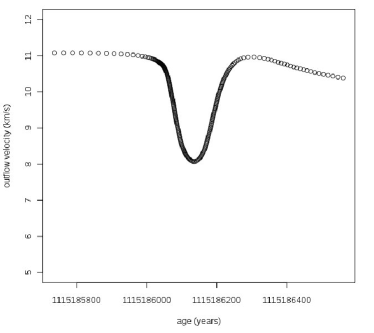
Figure 4: Zoom on last thermal pulse of Fig. 3.

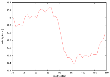
Figure 5: Temporal change over 40 periods of the outflow velocity in a hydrodynamical wind model – input parameters: $M=1\,M_{\sun}$, $T_{\text{eff}}=2600$ K, $L=10000\,L_{\sun}$, $P=640$ d, C/O=1.3, $\Delta v=5$ km s^-1.

As the most rapid and largest velocity change, we identify the about 200 years after a thermal pulse (TP), when the luminosity goes through a rapid dip. The outflow velocity corresponds here with a reduction of about 30%, on a timescale of only 50 years – see Fig. 4, which shows the final TP of Fig. 3 over a much smaller timespan.

This is, in expansion timescale, still a modest and, yet, not very fast velocity change. It does not exceed much the intrinsic, erratic fluctuations of the outflow of the dynamic wind models, of which Fig. 5 shows a typical example. These frequently reach or exceed 10%, on a timescale of only 10 years. We should therefore not expect to find any observable evidence for the TP-related changes of the wind velocity in the density structure of cool PN envelopes. Rather should the much larger relative changes of the mass-loss rate be held accountable for any distinguishable radial structure.

4 Discussion

Figure 6: Comparison with wind models by Mattsson et al. (2010) with C-O = 8.5 (corresponds to C/O $\sim$ 1.7); circles and triangles down: $\Delta v=4$ km s^-1, triangles up and diamonds: $\Delta v=6$ km s^-1, $M=0.75$ and $1\,M_{\sun}$, respectively.

How do our findings compare with results from other dust-driven wind models? Recently, Mattsson et al. (2010) published a grid of wind models with solar element abundances. The major difference of their models is the inclusion of non-grey radiative transfer. For comparison, Fig. 6 shows the outflow velocities of those models of Mattsson et al. (2010), which have a free carbon abundance C-O $=\log[(n_{\text{C}}-n_{\text{O}})/n_{\text{H}}]+12=8.5$ equivalent to a carbon-to-oxygen ratio of C/O $\sim 1.7$. This value is the best option to compare to our choice of C/O, since only a few models in their grid with C/O $\sim 1.35$, which is closer to our value, result in an outflow. Their $L/M$ ratio does not extend to high values because in their grid models with luminosities higher than 10 000 $L_{\sun}$ have only been calculated for masses larger than 1 $M_{\sun}$.

Furthermore, the models of Mattsson et al. (2010) show a wider spread in their outflow velocities – possibly due the influence of effective temperature. As for the mechanical energy input, we have set the piston velocity amplitude to 5 km s^-1. Hence, for Fig. 6 we used the models of Mattsson et al. (2010) with the closest choices in this respect, 4 and 6 km s^-1. The largest outflow velocity values seen in the figure correspond to the higher piston velocity.

Even though their model set seems to suggest a steeper exponent – as would our models restricted to the lower L/M range – our velocity relation overall is consistent with their grid, especially taking into account the wider spread of outflow velocity values in the Mattsson et al. (2010) models.

5 Conclusions

From the analysis of a consistent set of dust-driven wind models, we find that the velocity changes of the superwind can be parameterised by a simple dependence on $L/M$. In absolute terms, the related velocity changes are of a small nature, of the order of a fraction of the typical wind velocity. This is consistent with the very modest dependence of the velocity on $L$ and $M$ found by Habing et al. (1994), and both these findings are contrasted by the huge changes of the mass-loss rate (by several orders of magnitude).

Looking at the final phase of the superwind, systematic velocity changes are not exceeding the inherent short-term fluctuations of the dust-driven wind. And when a TP falls into this phase, there should only be a 30% velocity dip on a timescale of 50 years, which should still be difficult to extract from the density profile in view of the intrinsic erratic fluctuations of a dust-driven wind (over 10% on a timescale of 10 years).

Hence, we may conclude that the huge changes of the mass-loss rate in the history of a superwind, especially in the aftermath of a TP, are by far the dominant factor in shaping a present-day cool PN envelope, while changes in the velocity are hardly exceeding the natural fluctuation of a dust-driven wind. This find gives some support to a interpretation of cool PN envelopes in terms of a simple, constant outflow history, where the density profile mostly shows the progressively (in radial direction, that is with outflow age) diluted superwind and its mass-loss rate evolution.

References

- Bergeat & Chevallier (2005) Bergeat J., Chevallier L., 2005, A&A, 429, 235
- Cox (2001) Cox P., 2001, in “From optical to millimetric interferometry: scientific and technological challenges”, proceedings of the 36th Liège International Astrophysics Colloquium, Belgium, July 2–5, 2001, Eds.: Surdej J., Swings J.P., Caro D., Detal A., Université de Liège, 157
- Eggleton (1973) Eggleton P.P., 1973, MNRAS, 163, 179
- Fleischer et al. (1992) Fleischer A.J., Gauger A., Sedlmayr E., 1992, A&A, 266, 321
- Fong et al. (2006) Fong D., Meixner M., Sutton E.C., Zalucha A., Welch W.J., 2006, ApJ, 652, 1626
- Gail & Sedlmayr (1988) Gail H.-P., Sedlmayr E., 1988, A&A, 206, 153
- Gauger et al. (1990) Gauger A., Gail H.-P., Sedlmayr E., 1990, A&A, 235, 345
- Habing et al. (1994) Habing H.J., Tignon J., Tielens A.G.G.M., 1994, A&A, 286, 523
- Mattsson et al. (2010) Mattsson, L., Wahlin, R., Höfner, S., A&A, 509, 14
- Schirrmacher et al. (2003) Schirrmacher V., Woitke P., Sedlmayr E., 2003, A&A, 404, 267
- Phillips et al. (2009) Phillips J.P., Ramos-Larios G., Schröder K.-P., Verbena Contreras J.L., 2009, MNRAS, 399, 1126
- R Development Core Team (2008) R Development Core Team 2008, R: A Language and Environment for Statistical Computing, Vienna, Austria, ISBN 3-900051-07-0, http://www.R-project.org
- Renzini (1981) Renzini A. 1981, in: Iben Jr. I., Renzini A. (eds.), Physical Processes in Red Giants, Reidel, Dordrecht, p. 431
- Schönberner et al. (2005) Schönberner D., Jacob R., Steffen M., Perinotto M., Corradi R.L.M., Acker A. 2005, A&A 431, 963
- Schröder et al. (1999) Schröder K.-P., Winters J.M., Sedlmayr E., 1999, A&A, 349, 898
- Wachter et al. (2002) Wachter A., Schröder K.-P., Winters J.M., Arndt T.U., Sedlmayr E., 2002, A&A, 384, 452
- Weidemann (2000) Weidemann V. 2000, A&A 363, 647
- Weiss & Ferguson (2009) Weiss A., Ferguson J.W., 2009, A&A, 508, 1343
- Winters et al. (2000) Winters J.M., Le Bertre T., Jeong K.S., Helling Ch., Sedlmayr E., 2000, A&A, 361, 641