Reconstructing CMSSM parameters at the LHC with $\sqrt{s}={14}\,\text{TeV}$ via the golden decay channel

Abstract

We identify a benchmark point in the CMSSM’s heavy stau-coannihilation region, which is favored by experiments, and demonstrate that it could be accessible to the LHC at $\sqrt{s}={14}\,\text{TeV}$ with $300/\text{fb}$ of integrated luminosity via a golden decay measurement. With Monte-Carlo, we simulate sparticle production and subsequent golden decay at the event level and perform pseudo-measurements of sparticle masses from kinematic endpoints in invariant mass distributions. We find that two lightest neutralino masses and the first and second generation left-handed slepton and squark masses could be rather precisely measured with correlated uncertainties. We investigate whether from such measurements one could determine the CMSSM’s Lagrangian parameters by including a likelihood from our pseudo-measurements of sparticle masses in a Bayesian analysis of the CMSSM’s parameter space. We find that the CMSSM’s parameters can be accurately determined, with the exception of the common trilinear parameter. Experimental measurements of the relic density by Planck and the Higgs boson’s mass slightly improve this determination, especially for the common trilinear parameter. Finally, within our benchmark scenario, we show that the neutralino dark matter will be accessible to direct searches in future one tonne detectors.

I Introduction

Despite the absence of softly-broken supersymmetry (SUSY) in searches at the Large Hadron Collider (LHC)Aad et al. (2013); Chatrchyan et al. (2013a), SUSY remains a leading and attractive candidate for new physics beyond the Standard Model (SM).

The discovery by both ATLASChatrchyan et al. (2012) and CMSAad et al. (2012) of a Higgs-like boson with mass $m_{h}\simeq 126\,\text{GeV}$ indicates that the SUSY breaking scale is likely to be rather high, exceeding $1\,\text{TeV}$Roszkowski et al. (2012); Kowalska et al. (2013); Baer et al. (2013); Buchmueller et al. (2012). This, on the one hand, weakens naturalness arguments for SUSY but, on the other, is consistent with stringent bounds on superpartner masses from the LHC, and also is consistent with the fact that superpartners have not been observed yet, either directly or via loop effects in rare flavor changing processes.

In fact, within the framework of grand-unified (or, in other words, GUT-constrained) SUSY models, like the popular Constrained Minimal Supersymmetric Standard Model (CMSSM)Kane et al. (1994), the rather large Higgs boson mass favours a region of parameter space in which the lightest neutralino is higgsino-like with mass close to $1\,\text{TeV}$Strege et al. (2013); Cabrera et al. (2013); Kowalska et al. (2013). The same is true in the Non-Universal Higgs Model (NUHM)Roszkowski et al. (2011); Strege et al. (2013); Cabrera et al. (2013). This new high $M_{\rm SUSY}$ region appears at multi-TeV ranges of $m_{0}$ and $m_{1/2}$, in addition to the previously identified stau-coannihilation (SC), $A$-funnel (AF) and focus point/hyperbolic branch (FP/HB) regions. The favored regions are primarily determined by the relic density of the lightest neutralino, which is assumed to be dark matter.

Direct lower limits on SUSY masses from ATLAS and CMS have, at small $m_{0}\mathrel{\hbox to0.0pt{\lower 4.0pt\hbox{\hskip 1.0pt$\sim$}\hss}\raise 1.0pt\hbox{$<$}}400\,\text{GeV}$, pushed up the scalar mass parameter to $m_{1/2}\mathrel{\hbox to0.0pt{\lower 4.0pt\hbox{\hskip 1.0pt$\sim$}\hss}\raise 1.0pt\hbox{$>$}}850\,\text{GeV}$, while at multi-TeV $m_{0}$, the bound is much weaker, $m_{1/2}\mathrel{\hbox to0.0pt{\lower 4.0pt\hbox{\hskip 1.0pt$\sim$}\hss}\raise 1.0pt\hbox{$>$}}500\,\text{GeV}$ATL (2013); Aad et al. (2014). Measurements of the rare decay $\textrm{BR}\left(B_{s}\to\mu^{+}\mu^{-}\right)$ at LHCbAaij et al. (2013) and CMSChatrchyan et al. (2013b), which show no convincing deviations from the SM value, within constrained SUSY imply that the pseudoscalar Higgs boson, $A$, is heavy and also push the AF region up to $m_{1/2}\mathrel{\hbox to0.0pt{\lower 4.0pt\hbox{\hskip 1.0pt$\sim$}\hss}\raise 1.0pt\hbox{$>$}}1\,\text{TeV}$. In the FP/HB region at large $m_{0}$ one struggles to reproduce $m_{h}\sim 125\,\text{GeV}$Kowalska et al. (2013), and is now severely constrainedRoszkowski et al. (2014a) by new upper limits on the spin-independent WIMP-proton scattering cross section, $\sigma^{\rm SI}_{p}$, relevant to the direct detection of dark matter, from the LUX experimentAkerib et al. (2013, 2014).

Although the new $\sim 1\,\text{TeV}$ higgsino region reproduces the measured Higgs boson mass and the relic density, it lies in multi-TeV regions of both $m_{1/2}$ and $m_{0}$, and will be completely out of reach of the LHC, although within reach of dark matter searches in underground one tonne detectors and in the Cherenkov Telescope Array (CTA)Roszkowski et al. (2014a, b). Likewise, both in the AF and the FP/HB regions, all superpartners will be for the most part too heavy to be seen at the LHCBaer et al. (2012); Cohen et al. (2014); Fowlie and Raidal (2014); Roszkowski et al. (2014a).

The only cosmologically favored region that gives an acceptable Higgs boson mass and remains partially accessible to the LHC is the SC region. In fact, numerous studies prior to the LHC, e.g. Ruiz de Austri et al. (2006), found that the SC region was slightly preferred over the other ones because lighter sleptons and electroweakinos (EWinos) in loop corrections reduced the discrepancy with the SM value of the anomalous magnetic moment of the muonBennett et al. (2006). This motivates us to consider the possibility that at $\sqrt{s}={14}\,\text{TeV}$ the LHC might observe direct evidence for a model in the SC region of the CMSSM.

In preparation for the LHC operation, various groupsHinchliffe et al. (1997); Miller et al. (2006); Bachacou et al. (2000), including the ATLAS collaborationAad et al. (2009), simulated the precision with which the LHC could measure the masses of light sparticles in the CMSSM. Sparticle masses can be measured from kinematic endpoints in the invariant mass distributions of their decay productsGjelsten et al. (2004); Lester and Parker (2001) in the so-called “golden decay” channel (Fig. 1) which is a multi-stage squark decay,

$$\tilde{q}_{L}\to{\chi}^{0}_{2}q\to\tilde{\ell}^{\pm}\ell^{\mp}q\to\chi\ell^{+}\ell^{-}q,$$ (1)

where $\tilde{q}_{L}$ denotes a first- or second-generation left squark, $\chi^{0}_{1}=\chi$ and $\chi^{0}_{2}$ respectively the lightest and second-lightest neutralino and $\tilde{\ell}$ ($\ell$) a first- or second-generation slepton (lepton). The experimental signature for this chain will therefore be two leptons with opposite signs, a jet and missing energy. The jet will usually be hard but it might not be if the mass difference between the squark and the second-lightest neutralino happens to be small. The chain results in striking kinematic endpoints in the invariant mass distributions of the outgoing SM particles.

GoldenDecay (200,100) i1,i2,i3,i4

o1,o2,o3,o4

phantomi1,v1,v2,v3,o1 phantomi4,v4,v5,v6,o2

scalar, label=$\tilde{q}_{L}$i1,v1

fermion, label=$q$v1,v4 phantomv4,o4

gaugino, label=${\chi}^{0}_{2}$v1,v2

fermion, label=$\ell^{\mp}$, label.side=leftv2,v5 phantomv5,o3 scalar, label=$\tilde{\ell}_{L}$, label.side=leftv3,v2

fermion, label=$\ell^{\pm}$, label.side=rightv6,v3 phantomv6,o2 gaugino, label=$\chi$v3,o1

Figure 1: Feynman diagram for the golden decay.

Because the masses of the leptons can be neglected, the position of the edge of the leptons’ invariant mass distribution is a function of only the relevant sparticle masses;

$$m_{\ell\ell,\,\textrm{edge}}^{2}=\left(m_{{\chi}^{0}_{2}}^{2}-m_{\tilde{\ell}}^{2}\right)\left(\frac{m_{\tilde{\ell}}^{2}-m_{\chi}^{2}}{m_{\tilde{\ell}}^{2}}\right).$$ (2)

Measuring $m_{\ell\ell,\,\textrm{edge}}$ gives a relationship between $m_{{\chi}^{0}_{2}}$, $m_{\tilde{\ell}}$ and $m_{\chi}$. Measuring other invariant mass edges allows a model-independent reconstruction of all the masses involved in the decay chainBachacou et al. (2000). The squark flavors, however, will be indistinguishable, and a particular slepton might dominate the decay chain.

Squark production and subsequent decay via the golden decay was simulated in detail for particular CMSSM benchmark points, including SPS1aAllanach et al. (2002a) and ATLAS SU3Aad et al. (2009), from which the potential precision of sparticle mass measurements with a small integrated luminosity of $1/\text{fb}$ was estimatedAad et al. (2009); Gjelsten et al. (2004); Lester and Parker (2001); Allanach et al. (2002b, 2003); Lafaye et al. (2008); Bechtle et al. (2010).

InRoszkowski et al. (2010), the precision and reliability with which Lagrangian parameters for the SU3 point in the CMSSM could be determined were examined from a Bayesian perspective. Assuming a simple Gaussian approximation to the likelihood function describing golden decay measurements (but using a proper covariance matrix), it was found that the correct value of $m_{1/2}$ was reproduced very well, while the correct values of $m_{0}$, $\tan\beta$ and $A_{0}$ were reproduced increasingly poorly, in that order. In the case of the last variable, even the sign of $A_{0}$ remained undetermined. The effect of imposing in addition the neutralino’s relic density constraint was studied and found to be very important in improving the reconstruction of $m_{0}$ and, to a lesser extent, $\tan\beta$, while the error in $A_{0}$ remained large. Sensitivity to the choice of prior was also examined and found to be weak.

In an earlier version of this paper, the issue of parameter reconstruction of the SU3 point was extended using a similar methodology to models beyond the CMSSM: the Non-Universal Higgs Model (NUHM), the CMSSM with non-universal gaugino masses (CMSSM-NUG), both with two additional (although different) free parameters, and finally the MSSM with twelve free parameters, all defined at the EW scale. We propagated experimental uncertainties in sparticle masses to uncertainties in SUSY Lagrangian parameters with sophisticated statistical tools. We checked whether the benchmark point was accurately recovered, or whether additional information, from, for example, DM density would be required to recover the Lagrangian parameters, and whether one could distinguish various patterns of soft-breaking masses. Unsurprisingly, despite assuming more realistic uncertainties in computing the neutralino’s relic density, in the CMSSM we basically reproduced the results ofRoszkowski et al. (2010), while in the extended models we found that the prospects of reconstruction were generally poorer, although in some cases this was primarily so because the extended models relaxed gaugino mass unification rather than because of their larger number of free parameters. In the extended models prior dependence again became an issue. In a related paperAllanach and Dolan (2012) the SU3 point with the CMSSM mass spectrum was used to examine whether golden decay measurements at the LHC could be accommodated instead by some other SUSY breaking scenarios, with a generally positive conclusion.

Unfortunately, the SU3 point, along with most light SUSY scenarios, was in fact excluded by direct searches for SUSY at the LHC at $\sqrt{s}={7}\,\text{TeV}$ Chatrchyan et al. (2013a); Aad et al. (2013). Light SUSY scenarios are also disfavored by the discovery of a Higgs boson with a mass $m_{h}\sim 126\,\text{GeV}$Chatrchyan et al. (2012); Aad et al. (2012), since heavy stops are needed to produce large radiative corrections to the Higgs boson mass; see, e.g.,Kowalska et al. (2013).

In this paper we return to anticipating that SUSY might be residing not far above the current lower limits and that, after its hiatus, the LHC might discover SUSY in its $\sqrt{s}={14}\,\text{TeV}$ phaseBaer et al. (2012). To this end, and in light of our earlier discussion, we select a new benchmark point in the SC region allowed by current LHC bounds, which we specify below. We ask, if nature is described by a CMSSM scenario, compatible with previous direct searches and with the Higgs boson observation, how well might one be able to measure sparticle masses at the LHC and, subsequently, how well might one be able to determine Lagrangian parameters and make predictions for other observable quantities.

In light of LHC results the CMSSM might appear less natural than beforeFowlie (2014); however, it correctly reproduces both the Higgs boson mass and the DM relic abundance in the “unnatural” multi-TeV regions of mass parameters. It also remains compatible with all experimental data, with the exception of the anomalous magnetic moment of the muon.

Our paper is organized as follows; in Sec. II, we construct our scenario, in Sec. III, we describe the Monte-Carlo simulation of sparticle mass measurements via the kinematic endpoints of a golden decay; in Sec. IV, we recapitulate our statistical methodology, with which we propagate uncertainties in hypothetical sparticle mass measurements to uncertainties in Lagrangian parameters, and in Sec. V we present our results.

II Benchmark point and scenario

First we identify a CMSSM parameter point that is compatible with existing constraints and that might be found early in the LHC $\sqrt{s}={14}\,\text{TeV}$ run via the golden decay. In addition to the CMSSM parameters, there are SM nuisance parameters with experimental uncertainties that can impact SUSY phenomenology: the top pole mass, $M_{t}$, the bottom quark running mass, $m_{b}(m_{b})^{\overline{MS}}$, and the strong and electromagnetic couplings, $\alpha_{s}(M_{Z})^{\overline{MS}}$ and $1/\alpha_{\mathrm{em}}(M_{Z})^{\overline{MS}}$ respectively. Our complete set of parameters is, therefore,

$$m=\left(m_{1/2},m_{0},A_{0},\tan\beta,\text{sign}\,\mu,M_{t},m_{b}(m_{b})^{\overline{MS}},\alpha_{s}(M_{Z})^{\overline{MS}},1/\alpha_{\mathrm{em}}(M_{Z})^{\overline{MS}}\right).$$ (3)

Our desiderata are that our benchmark point exhibits a golden decay, predicts a relic density in agreement with PlanckAde et al. (2014) and a correct Higgs boson mass, $m_{h}\sim 126\,\text{GeV}$, within theory errors, and is consistent with constraints from current direct SUSY searches.

For a squark to cascade via the golden decay a particular sparticle mass hierarchy is required, and for the process to be significant necessitates other (spoiler) decay modes to be suppressed and kinematic phase space to be moderateGjelsten et al. (2004). We thus require that the gluino is heavier than the squarks, shutting the $\tilde{q}\to q\tilde{g}$ spoiler mode. We obviously require that squarks are heavier than the second lightest neutralino, which is typical in the CMSSM. We require that the second lightest neutralino is heavier than a slepton; although the second lightest neutralino could reach an identical final state via a three-body decay mediated by a $Z$-boson, the kinematic endpoints would be ruined. In fact, we require that it is at least $50\,\text{GeV}$ heavier, so that the decay is not suppressed by small phase-space.

Because we wish to simultaneously agree with DM density measurementsAde et al. (2014), our benchmark must invoke a particular mechanism to annihilate DM in the early Universe. The aforementioned requirement, that $m_{{\chi}^{0}_{2}}>m_{\tilde{\ell}}+50\,\text{GeV}$, limits the CMSSM parameter space from which we can select our benchmark to regions in which $m_{1/2}\gg m_{0}$. This requirement in conjunction with that from the relic density, means we can pick only from the SC region of CMSSM parameter space, in which neutralinos and staus are almost degenerate in mass and efficiently coannihilate. We, however, require that the neutralino and stau masses differ by more than the $\tau$-lepton mass to avoid limits from long-lived stausCitron et al. (2013). Within the SC region, current direct SUSY search constraints impose $m_{1/2}\mathrel{\hbox to0.0pt{\lower 4.0pt\hbox{\hskip 1.0pt$\sim$}\hss}\raise 1.0pt\hbox{$>$}}850\,\text{GeV}$ATL (2013); Aad et al. (2014).

We located our benchmark point by conducting a local scan within a small part of the parameter space in the SC region with the Minuit algorithmJames and Roos (1975). We fixed $m_{1/2}=900\,\text{GeV}$ to maximize production cross sections but still stay above the lightest permitted value inATL (2013); Aad et al. (2014), and varied the CMSSM’s three other continuous parameters and the SM top pole mass to minimize a $\chi^{2}$-function from nine experiments, including Higgs boson, dark matter and $B$-physics experiments. This way we found a local minimum which we accepted as our benchmark point. The point and its mass spectrum are shown in Table 1 and Table 2, respectively, and its mass spectrum is plotted in Fig. 2. Our benchmark’s branching ratios are such that a golden decay begins most often with a left-handed first- or second-generation squark, and proceeds via a left-handed first- or second-generation slepton. At the electroweak scale, our benchmark has $\mu\sim 1.5\,\text{TeV}\gg M_{1},M_{2}$. The lightest and second-lightest neutralinos are approximately entirely bino- and wino-like, respectively. Our benchmark top pole mass $M_{t}=174.3\,\text{GeV}$ is larger than but in agreement with its world average inBeringer et al. (2012), especially if one follows caveats regarding the interpretation of top mass measurements as measurements of the pole mass.

Parameter	Description	Benchmark value
$m_{0}$	Unified scalar mass	$315$ GeV
$m_{1/2}$	Unified gaugino mass	$900$ GeV
$A_{0}$	Unified trilinear	$-2550$ GeV
$\tan\beta$	Ratio of Higgs vevs	$11.0$
$\text{sign}\,\mu$	Sign of Higgs parameter	$+1$
$M_{t}$	Top pole mass	$174.3$ GeV
$m_{b}(m_{b})^{\overline{MS}}$	Bottom running mass	$4.18$ GeV
$1/\alpha_{\mathrm{em}}(M_{Z})^{\overline{MS}}$	Inverse of EM coupling	$127.944$
$\alpha_{s}(M_{Z})^{\overline{MS}}$	Strong coupling	$0.1184$

Table 1: Our benchmark CMSSM parameters with three significant figures and benchmark SM nuisance parameters. The SM nuisance parameters are the world averages inBeringer et al. (2012), with the exception of $M_{t}$.

Particle Mass (GeV):
${\chi}^{0}_{1}=\chi$	$382.8$	$\tilde{e}_{L}$	$679.8$	$\tilde{d}_{L}$	$1835$	$h$	$124.1$
${\chi}^{0}_{2}$	$728.7$	$\tilde{e}_{R}$	$463.4$	$\tilde{d}_{R}$	$1754$	$H$	$1741$
${\chi}^{0}_{3}$	$1645$	$\tilde{\nu}_{e}$	$675.1$	$\tilde{u}_{L}$	$1834$	$A$	$1742$
${\chi}^{0}_{4}$	$1649$	$\tilde{\tau}_{1}$	$384.6$	$\tilde{u}_{R}$	$1762$	$H^{\pm}$	$1744$
${\chi}^{\pm}_{1}$	$728.9$	$\tilde{\tau}_{2}$	$659.9$	$\tilde{b}_{1}$	$1509$
${\chi}^{\pm}_{2}$	$1649$	$\tilde{\nu}_{\tau}$	$651.4$	$\tilde{b}_{2}$	$1726$
$\tilde{g}$	$1985$			$\tilde{t}_{1}$	$984.1$
				$\tilde{t}_{2}$	$1552$

Table 2: The particle mass spectrum for our CMSSM benchmark, calculated with softsusy-3.3.7Allanach (2002). The first- and second-generation sparticles are approximately degenerate in mass.

Since our benchmark point lies in the SC region, $m_{\tilde{\tau}_{1}}\approx m_{\chi}$ (Table 2), though their masses are chosen to differ by more than the $\tau$-lepton mass to avoid limits from long-lived stausCitron et al. (2013). With this restriction, and $m_{1/2}\mathrel{\hbox to0.0pt{\lower 4.0pt\hbox{\hskip 1.0pt$\sim$}\hss}\raise 1.0pt\hbox{$>$}}850\,\text{GeV}$ from direct searches, the relic density cannot be reduced via SC to the Planck measurement, $\Omega h^{2}=0.1196$; we can go as far down as $\Omega h^{2}=0.1390$Belanger et al. (2011).

We check, however, that our benchmark point is in global agreement with experimental constraints. In an ensemble of measurements, there is an appreciable chance of a discrepant measurement. Our benchmark point satisfied nine experimental measurements: the Higgs boson mass, dark matter relic density, $b\rightarrow s\gamma$, $B_{u}\rightarrow\tau\nu$, $B_{s}\to\mu^{+}\mu^{-}$, $m_{W}$, $\sin^{2}\theta_{\mathrm{eff}}$, $M_{t}$ and $\Delta M_{B_{s}}$., having fitted four parameters, with $\chi^{2}=8.8$. Assuming that our benchmark point describes nature, the probability of obtaining by chance $\chi^{2}\geq 8.8$, the $p$-value, is $12\%$. Our benchmark point is therefore acceptable.

Figure 2: The mass spectrum for our benchmark point, with the golden decay indicated by arrows, calculated with softsusy-3.3.7Allanach (2002). Because the first- and second-generation sparticles are approximately degenerate in mass, they are plotted only once each.

III Simulating golden decay measurements

One can consider the Minkowski-square of sums of the four-momenta of the visible SM decay products in Eq. 1, resulting in four invariant masses:

$$m_{\ell\ell}^{2} =(p_{\ell_{\text{near}}}+p_{\ell_{\text{far}}})^{2},$$ (4)

$$m_{\ell_{\text{near}}q}^{2} =(p_{q}+p_{\ell_{\text{near}}})^{2},$$

$$m_{\ell_{\text{far}}q}^{2} =(p_{q}+p_{\ell_{\text{far}}})^{2},$$

$$m_{\ell\ell q}^{2} =(p_{q}+p_{\ell_{\text{near}}}+p_{\ell_{\text{far}}})^{2},$$

where $\ell_{\text{near}}$ and $\ell_{\text{far}}$ are the first and second lepton produced in a cascade, respectively. Because at the LHC one cannot identify the lepton’s origins, we instead consider the maximum and minimum invariant mass from the quark-lepton combinations. Four kinematic endpoints are predicted by calculating these Minkowski-squares and maximizing with respect to angular distributions. The clearest endpoint is that from $m_{\ell\ell}^{2}$, because it has no spin corrections as it is mediated by a scalar. The locations of these four kinematic features can be exactly predicted from the sparticle mass spectrum; the formulas were derived inLester and Parker (2001); Gjelsten et al. (2004).

We simulated 10,000 SUSY events at $\sqrt{s}={14}\,\text{TeV}$ with our benchmark point with the Pythia 8.1Sjostrand et al. (2008) Monte-Carlo event generator. This number of events is equivalent to $\sim 100/\text{fb}$, which could be collected in $\sim 2$ years at the LHC. We applied geometrical cuts to insure events were inside the detector, but otherwise applied no detector simulation. We selected events with an opposite-sign same-flavor lepton pair, at least two jets (with standard definitions for leptons and jets) and missing energy. We required that the hardest jet had transverse momentum $p_{T}>100\,\text{GeV}$ and removed the $Z$-boson peak in the leptonic invariant mass distribution by vetoing $89\,\text{GeV}<m_{\ell\ell}<95\,\text{GeV}$.

In the CMSSM, because of $R$-parity conservation, colored sparticles ought to be produced in pairs in QCD interactions at the LHC; each side of a SUSY QCD event should contain a hard jet. We had to decide which of the two hardest jets was associated with the golden decay. If we were looking for a high (low) edge in an invariant mass distribution, we chose the jet that minimized (maximized) that invariant mass. This choice was conservative; invariant mass distributions were never populated beyond their expected edges because of contamination with the jet from the opposite side of the decay chain.

We produced histograms for our selected events according to the invariant masses in Eq. 4 with ROOTBrun and Rademakers (1997). The resulting invariant mass distributions exhibited the expected kinematic features. With Minuit, we extracted their positions by fitting simple curves to the distributions with a least-squares technique, with Poisson $\sqrt{N}$ error bars in our histograms. This resulted in uncorrelated pseudo-measurements of four endpoints with statistical errors. Because the statistical error is dominant, we neglected systematic errors in our analysis.

To find sparticle masses from the endpoints, we used formulas for the endpoints inLester and Parker (2001); Gjelsten et al. (2004). The measurable masses are:

$$m_{\chi},m_{{\chi}^{0}_{2}},m_{\tilde{q}},m_{\tilde{\ell}},$$ (5)

where $m_{\tilde{q}}$ and $m_{\tilde{\ell}}$ are effective squark and slepton masses that dominate the golden decay. In our earlier SU3 studies, the effective squark mass was the average of the first- and second-generation squark masses, because at the LHC their productive cross sections are substantial and one cannot easily distinguish first- and second-generation squarks, and the effective slepton mass was that of the lightest slepton, which was assumed to dominate the decay chain;

$$m_{\tilde{q}} = \frac{1}{8}\left(m_{\tilde{u}_{R}}+m_{\tilde{u}_{L}}+m_{\tilde{d}_{R}}+m_{\tilde{d}_{L}}+m_{\tilde{s}_{R}}+m_{\tilde{s}_{L}}+m_{\tilde{c}_{R}}+m_{\tilde{c}_{L}}\right),$$ (6)

$$m_{\tilde{\ell}} = \min\left(m_{\tilde{e}_{R}},m_{\tilde{e}_{L}},m_{\tilde{\mu}_{R}},m_{\tilde{\mu}_{L}},m_{\tilde{\tau}_{1}},m_{\tilde{\tau}_{2}}\right).$$ (7)

For our current study we refined our definitions. The effective squark mass was the average of only left-handed first- and second-generation squarks, and the effective slepton mass was the average left-handed selectron and smuon masses;

$$m_{\tilde{q}} = \frac{1}{4}\left(m_{\tilde{u}_{L}}+m_{\tilde{d}_{L}}+m_{\tilde{s}_{L}}+m_{\tilde{c}_{L}}\right),$$ (8)

$$m_{\tilde{\ell}} = \frac{1}{2}\left(m_{\tilde{e}_{L}}+m_{\tilde{\mu}_{L}}\right).$$ (9)

Because the second lightest neutralino is wino-like for our benchmark point, the golden decay is dominated by left-handed sparticles. Because taus cannot be reliably detected, they were omitted from our analysis. The definitions are model dependent; in relaxed models, the golden decay might be dominated by other sparticles.

Rather than using the inverted formulas for sparticle masses, however, we fitted sparticle masses to our pseudo-measurements of the endpoints by minimizing a $\chi^{2}$-function with Minuit. The Migrad minimization algorithm in Minuit is a quasi-Newton method, which utilizes derivatives of the $\chi^{2}$-function. The matrix of second derivatives of the $\chi^{2}$-function is proportional to the inverse covariance matrix. The resulting covariance matrix, defined by ${\sigma}_{ij}={\sigma}_{ji}=\text{E}(X_{i})\text{E}(X_{j})-\text{E}(X_{i}X_{j})$, where E denotes an expectation value and

$$X=(m_{{\chi}^{0}_{1}},m_{\tilde{\ell}},m_{{\chi}^{0}_{2}},m_{\tilde{q}})^{T},$$ (10)

is

$$\sigma=\begin{pmatrix}132.0&18.4&31.9&175.8\\ \cdot&25.5&24.2&21.3\\ \cdot&\cdot&24.8&39.6\\ \cdot&\cdot&\cdot&401.1\\ \end{pmatrix},$$ (11)

in units of $(\text{GeV})^{2}$. The non-zero off-diagonal covariance matrix elements indicate that the mass measurements are correlated. The $\chi^{2}$-function associated with the covariance matrix is

$$\chi^{2}=(X-X_{\text{BM}})^{T}\sigma^{-1}(X-X_{\text{BM}})$$ (12)

where $X_{\text{BM}}$ stands for $X$ evaluated at our benchmark point, i.e., the expected values of $X$.

For insight, we diagonalize the inverse of this matrix to obtain the orthonormal eigenvectors, the combinations of masses that can be independently measured, and their eigenvalues. For clarity, let us make our original basis, $(\hat{e}_{m_{{\chi}^{0}_{1}}},\hat{e}_{m_{\tilde{\ell}}},\hat{e}_{m_{{\chi}^{0}_{2}}}\,\hat{e}_{m_{\tilde{q}}})$, explicit;

$$X=m_{{\chi}^{0}_{1}}\cdot\hat{e}_{m_{{\chi}^{0}_{1}}}+m_{\tilde{\ell}}\cdot\hat{e}_{m_{\tilde{\ell}}}+m_{{\chi}^{0}_{2}}\cdot\hat{e}_{m_{{\chi}^{0}_{2}}}+m_{\tilde{q}}\cdot\hat{e}_{m_{\tilde{q}}}.$$ (13)

To diagonalize the inverse covariance matrix, we find the orthogonal matrix $V$ such that $V^{T}\sigma^{-1}V$ is diagonal. The errors for the independent mass combinations are the eigenvalues of $\sigma^{-1}$, i.e., the entries of $V^{T}\sigma^{-1}V$;

$$V\,\sigma^{-1}\,V^{T}\approx\text{diag}\left[(0.3\,\text{GeV})^{-2},(5.6\,\text{GeV})^{-2},(7.5\,\text{GeV})^{-2},(22.3\,\text{GeV})^{-2}\right],$$ (14)

and the independent combinations of masses are the eigenvectors of $\sigma^{-1}$, i.e., the columns of the orthogonal matrix that diagonalizes our covariance matrix;

$$V_{1i} =0.1\cdot\hat{e}_{m_{{\chi}^{0}_{1}}}+0.7\cdot\hat{e}_{m_{\tilde{\ell}}}-0.8\cdot\hat{e}_{m_{{\chi}^{0}_{2}}}+0.0\cdot\hat{e}_{m_{\tilde{q}}},$$ (15)

$$V_{2i} =0.6\cdot\hat{e}_{m_{{\chi}^{0}_{1}}}-0.6\cdot\hat{e}_{m_{\tilde{\ell}}}-0.4\cdot\hat{e}_{m_{{\chi}^{0}_{2}}}-0.2\cdot\hat{e}_{m_{\tilde{q}}},$$

$$V_{3i} =0.6\cdot\hat{e}_{m_{{\chi}^{0}_{1}}}-0.4\cdot\hat{e}_{m_{\tilde{\ell}}}-0.5\cdot\hat{e}_{m_{{\chi}^{0}_{2}}}+0.4\cdot\hat{e}_{m_{\tilde{q}}},$$

$$V_{4i} =0.4\cdot\hat{e}_{m_{{\chi}^{0}_{1}}}+0.1\cdot\hat{e}_{m_{\tilde{\ell}}}+0.1\cdot\hat{e}_{m_{{\chi}^{0}_{2}}}+0.9\cdot\hat{e}_{m_{\tilde{q}}}.$$

The combinations of masses that can be independently measured are:

$$V_{1i}X_{i} =0.1\cdot m_{{\chi}^{0}_{1}}+0.7\cdot m_{\tilde{\ell}}-0.8\cdot m_{{\chi}^{0}_{2}}+0.0\cdot m_{\tilde{q}}\approx\frac{1}{\sqrt{2}}(m_{\tilde{\ell}}-m_{{\chi}^{0}_{2}}),$$ (16)

$$V_{2i}X_{i} =0.6\cdot m_{{\chi}^{0}_{1}}-0.6\cdot m_{\tilde{\ell}}-0.4\cdot m_{{\chi}^{0}_{2}}-0.2\cdot m_{\tilde{q}},$$

$$V_{3i}X_{i} =0.6\cdot m_{{\chi}^{0}_{1}}-0.4\cdot m_{\tilde{\ell}}-0.5\cdot m_{{\chi}^{0}_{2}}+0.4\cdot m_{\tilde{q}},$$

$$V_{4i}X_{i} =0.4\cdot m_{{\chi}^{0}_{1}}+0.1\cdot m_{\tilde{\ell}}+0.1\cdot m_{{\chi}^{0}_{2}}+0.9\cdot m_{\tilde{q}}\approx m_{\tilde{q}}.$$

It will later be of significance that the combination $(m_{\tilde{\ell}}-m_{{\chi}^{0}_{2}})$ has by far the smallest experimental uncertainty. We assume that the expected measured endpoints are our benchmark’s endpoints (i.e., that there is no bias), and that consequently, the expected extracted masses are our benchmark’s sparticle masses.

IV Statistical methodology

We first recapitulate our Bayesian methodology; more details can be found in, e.g.,Roszkowski et al. (2007); Fowlie et al. (2012). At each point $m=(m_{0},m_{1/2},A_{0},\tan\beta)$ in the CMSSM’s parameter space we calculate our observables. We want to know the posterior probability density function (pdf) of the CMSSM parameters given the experimental data $d$. We find this via Bayes’ theorem,

$$p(m|d) =\frac{p(d|m)\,p(m)}{p({d})},$$

$$=\frac{\mathcal{L}\left(m\right)p(m)}{\mathcal{Z}},$$ (17)

where $\mathcal{L}\left(m\right)$ is the likelihood function, the probability of obtaining data $d$ for our observables at a given point $m$; $\pi\left(m\right)$ is the prior probability density function, our prior belief in the CMSSM parameter space and nuisance parameters; $\mathcal{Z}$ is the Bayesian evidence, which is just a normalization factor in this instance; and $p(m|d)$ is the posterior pdf, the object that we wish to find, given the experimental data $d$.

We will obtain the posterior with the nested sampling algorithmSkilling (2006), implemented in the MultiNest computer packageFeroz and Hobson (2008); Feroz et al. (2009), by supplying the algorithm with our chosen priors for the CMSSM parameters and with our likelihood functions for the experimental data. We will inspect the posterior by plotting $68\%$ and $95\%$ credible regions on two-dimensional planes of the CMSSM parameter space. We find such regions by first marginalizing the posterior over the other two CMSSM parameters and over all SM nuisance parameters,

$$p\left(x_{1},x_{2}|d\right)=\int p\left(m|d\right)\,\text{d}x_{3}\text{d}x_{4}\ldots,$$ (18)

and second finding the smallest regions of the $\left(x_{1},x_{2}\right)$ plane that contain $68\%$ and $95\%$ of the marginalised posterior; these are the credible regions,

$$\int p\left(x_{1},x_{2}|d\right)\text{d}x_{1}\text{d}x_{2}=0.68\text{\leavevmode\nobreak\ or\leavevmode\nobreak\ }0.95.$$ (19)

We will consider three sets of experimental data:

1. hypothetical golden decay sparticle mass measurements described in Sec. III (LHC);

2. Higgs boson mass data (Higgs);

3. dark matter relic density (Planck).

Our likelihood function for LHC, described in Sec. III, is a multivariate Gaussian, reflecting the correlations in the sparticle mass measurements,

$$\mathcal{L}\left(\texttt{LHC}\right)=\exp\left[-0.5\,(X-X_{\text{BM}})^{T}\sigma^{-1}(X-X_{\text{BM}})\right],$$ (20)

where ${\sigma}^{-1}$ is the inverse of the covariance matrix (note that this is already a squared quantity) obtained in Sec. III, and $X$, already defined above, is the set of the measurable sparticles masses evaluated at the CMSSM point in question, whilst the index BM denotes that the quantity is evaluated at our benchmark point.

We calculate the sparticle mass spectrum and the Higgs boson mass $m_{h}$ with softsusy 3-3.7Allanach (2002), and the relic density $\Omega_{\chi}h^{2}$ of the lightest neutralino with micromegas-2.4.5Belanger et al. (2011). These quantities are compared with measurements through likelihood functions, which are assumed to be Gaussian, though we include in quadrature theoretical errors in the CMSSM predictions for these observables of $3\,\text{GeV}$Allanach et al. (2004a) and $10\%$Allanach et al. (2004b, c), respectively:

$$\mathcal{L}\left(\texttt{Higgs}\right) =\exp\left[-\frac{\left(125.8\,\text{GeV}-m_{h}\right)^{2}}{2[(0.6\,\text{GeV})^{2}+(3\,\text{GeV})^{2}]}\right],$$

$$\mathcal{L}\left(\texttt{Planck}\right) =\exp\left[-\frac{\left(0.1196-\Omega_{\chi}h^{2}\right)^{2}}{2[0.0031^{2}+(0.1\Omega_{\chi}h^{2})^{2}]}\right],$$ (21)

where the means and standard deviations are those reported by CMSChatrchyan et al. (2012); Aad et al. (2012) and by PlanckAde et al. (2014), respectively. The relic density of $\Omega_{\chi}h^{2}=0.1390$ and Higgs boson mass of $124.1\,\text{GeV}$ calculated at our benchmark point agree, within theoretical and experimental errors, with the Planck measurementAde et al. (2014) $\Omega h^{2}=0.1196$ and from the CMS measurementChatrchyan et al. (2012); Aad et al. (2012) of $125.8\,\text{GeV}$, respectively. We, however, include in our likelihoods the measured relic density and measured Higgs boson mass, rather than our benchmark’s values. This is not a fault; it reflects the experimental and theoretical uncertainties in these measurements and any biases that they might introduce.

We consider three cases, by adding these data one by one:

1. golden decay pseudo-data only, $\mathcal{L}=\mathcal{L}\left(\texttt{LHC}\right)$;

2. golden decay and Higgs boson mass data, $\mathcal{L}=\mathcal{L}\left(\texttt{LHC}\right)\cdot\mathcal{L}\left(\texttt{Higgs}\right)$;

3. golden decay, Higgs boson mass and relic density data, $\mathcal{L}=\mathcal{L}\left(\texttt{LHC}\right)\cdot\mathcal{L}\left(\texttt{Higgs}\right)\cdot\mathcal{L}\left(\texttt{Planck}\right)$.

Our choice of priors for the CMSSM parameters is slightly moot; our likelihood $\mathcal{L}\left(\texttt{LHC}\right)$ ought to be informative enough to overcome different, sensible choices of priorTrotta et al. (2008). We choose flat priors for the CMSSM parameters that evenly weight the parameter space, listed in Table 3, but expect our posterior to be independent of this choice.

In general we should also vary the SM nuisance parameters but their inclusion would be computationally expensive and would have limited impact in our scenario. We fix these parameters to the weighted averages of their experimental values inBeringer et al. (2012), rather than our benchmark point’s values. Our benchmark point’s top mass in Table 1, however, is slightly larger than the weighted average to maximise the Higgs boson mass. In our scenario, one would know only the measured top mass and not our benchmark point’s top mass.

Parameter	Prior range	Distribution
$m_{0}$	$(0.1,\,4)\,\text{TeV}$	Flat
$m_{1/2}$	$(0.1,\,2)\,\text{TeV}$	Flat
$A_{0}$	$(-4,\,4)\,\text{TeV}$	Flat
$\tan\beta$	$(3,\,62)$	Flat
$\text{sign}\,\mu$	$+1$	Fixed
$M_{t}$	$173.5$ GeV	Fixed
$m_{b}(m_{b})^{\overline{MS}}$	$4.18$ GeV	Fixed
$1/\alpha_{\mathrm{em}}(M_{Z})^{\overline{MS}}$	$127.944$	Fixed
$\alpha_{s}(M_{Z})^{\overline{MS}}$	$0.1184$	Fixed

Table 3: Our prior distributions for the CMSSM parameters in our calculation of the posterior pdf for the CMSSM. The SM nuisance parameters are fixed to their world averages inBeringer et al. (2012).

V Results

We successfully found the posterior pdf and subsequently the credible regions for the CMSSM in three cases: our hypothetical LHC likelihood only, our hypothetical LHC likelihood and a likelihood from the Higgs mass measurement, and our hypothetical LHC likelihood and likelihoods from the Higgs mass measurement and the Planck relic density measurement. To highlight the impact and necessity of additional information in parameter reconstruction, we discuss our results parameter plane by parameter plane in all three cases, rather than likelihood by likelihood.

(a)

(b)

(c)

Figure 3: The $68\%$ (dark blue) and $95\%$ (light blue) credible regions of the $(m_{0},\,m_{1/2})$ plane of the CMSSM, adding the data one by one from left to right. The parameters $\tan\beta$ and $A_{0}$ were marginalised. Our benchmark point is marked with a red diamond and the posterior mean is marked with a black circle. The bin limits are identical to the plot limits with $25$ bins per dimension.

We first consider the $(m_{0},\,m_{1/2})$ plane of the CMSSM in Fig. 3, showing all three cases from left to right. (The corresponding results in the $(A_{0},\,\tan\beta)$ plane of the CMSSM are shown below in Fig. 4.) Note the narrow $60\,\text{GeV}\times 60\,\text{GeV}$ scales shown; the parameters are reconstructed at the $95\%$ level to within $\lesssim 20\%$. Reconstruction of $(m_{0},\,m_{1/2})$ with only LHC is somewhat successful; a single $95\%$ mode is recovered, which envelopes the benchmark point. Our benchmark point is, however, outside our $68\%$ credible region. Two orthogonal directions in the parameter space are visible: the anti-diagonal $m_{0}-m_{1/2}$ direction and the diagonal $m_{0}+m_{1/2}$ direction, which correspond to the first and second eigenvectors of our covariance matrix in Eq. 15.

To see that the $m_{0}-m_{1/2}$ direction corresponds to the first eigenvector, recall that the first eigenvector corresponded to the $m_{\tilde{\ell}}-m_{{\chi}^{0}_{2}}$ combination of masses with a small $0.3\,\text{GeV}$ uncertainty. That combination is approximately unchanged if $m_{0}$ and $m_{1/2}$ are simultaneously increased by $\sim 10\,\text{GeV}$, as each mass is increased by a similar amount, since $m_{\tilde{\ell}}\approx 0.8m_{0}$. This dominant measurement, therefore, constrains our credible regions to a line $m_{1/2}\propto m_{0}$, with a breadth proportional to the $0.3\,\text{GeV}$ uncertainty. The $m_{0}-m_{1/2}$ direction, perpendicular to this line, is constrained.

To see that the $m_{0}+m_{1/2}$ direction corresponds to the second eigenvector, recognise there is no approximate cancellation in $V_{2i}X_{i}$ if $m_{1/2}$ and $m_{0}$ are simultaneously increased, but that cancellations are possible if $m_{1/2}$ is increased and $m_{0}$ is decreased. This measurement, therefore, constrains our credible regions to a line $m_{1/2}\propto-m_{0}$, with a breadth proportional to the $5.6\,\text{GeV}$ uncertainty. The $m_{0}+m_{1/2}$ direction, perpendicular to this line, is constrained.

The third and fourth eigenvectors are negligible; the third because that combination of masses changes relatively slowly with $(m_{0},\,m_{1/2})$, because of cancellations in $m_{{\chi}^{0}_{1}}-m_{{\chi}^{0}_{2}}$ and $m_{\tilde{\ell}}-m_{\tilde{q}}$, and the fourth because its associated uncertainty is large.

Because of its small associated uncertainty of $0.3\,\text{GeV}$, we might expect that the anti-diagonal $m_{0}-m_{1/2}$ direction is more constrained than the diagonal $m_{0}+m_{1/2}$ direction on the $(m_{0},\,m_{1/2})$ plane. The second-lightest neutralino mass, however, can be tuned independently of the slepton mass by $\sim 10\,\text{GeV}$ by tuning $A_{0}$ to increase the second-lightest neutralino’s higgsino component. Note that in Fig. 4a $A_{0}$ is not well constrained. This freedom broadens the credible region in the $m_{0}-m_{1/2}$ direction. One can decrease $m_{0}$ from its benchmark and increase $m_{1/2}$ from its benchmark, to keep $m_{\tilde{\ell}}$ constant, but achieve $m_{{\chi}^{0}_{2}}-m_{\tilde{\ell}}$ similar to its pseudo-measurement by increasing $A_{0}$ from its benchmark which decreases $m_{{\chi}^{0}_{2}}$ to compensate for the increase in $m_{1/2}$. One cannot compensate for increased $m_{0}$ and decreased $m_{1/2}$ by decreasing $A_{0}$, however, because ${\chi}^{0}_{2}$ mass is already saturated at our benchmark, i.e. it is already entirely wino-like. This is why the $m_{0}+m_{1/2}$ direction is more constrained.

The credible regions shrink successively as the data is added, though two orthogonal directions in the parameter space remain visible. The $m_{0}+m_{1/2}$ direction of the credible region is only marginally shrunk by additional data, whereas the $m_{0}-m_{1/2}$ direction of the credible region is squashed. When we add Higgs, $A_{0}$ must be $\lesssim 0.5\,\text{TeV}$ (see Fig. 4b) to increase the Higgs boson mass via maximal mixing. The left-hand side of the $(m_{0},\,m_{1/2})$ credible region, which achieved agreement with LHC via $A_{0}\sim 0$, is excluded and absent in Fig. 3b. Increases in Higgs boson mass from increasing $m_{1/2}$ and $m_{0}$ to increase stop masses are negligible. Indeed, varying $m_{1/2}$ by $50\,\text{GeV}$ ($10\,\text{GeV}$) of our benchmark point changes the Higgs boson mass by only $0.1\,\text{GeV}$ ($0.0\,\text{GeV}$), which is negligible compared with the $3\,\text{GeV}$ theory error in $m_{h}$.

When we add Planck, we enforce $m_{\tilde{\tau}_{1}}\approx m_{{\chi}^{0}_{1}}$, so that staus and neutralinos coannihilate effectively and reduce the relic density to the Planck value. This further squashes the $m_{0}-m_{1/2}$ direction of the credible region. Furthermore, Planck requires that $(A_{0},\,\tan\beta)$ are tuned so that the stau mixing results in $m_{\tilde{\tau}_{1}}\approx m_{{\chi}^{0}_{1}}$, reducing the freedom to tune the neutralino masses with $A_{0}$ for the LHC pseudo-measurements (compare Fig. 4c). This is rather fortunate; Higgs and Planck constrain the direction of parameter space that was poorly constrained by LHC, enhancing the impact of this additional information.

The complicated dependence of neutralino and stau masses on $A_{0}$ results in bias in our credible regions and posterior means. In Fig. 3, in the $m_{0}-m_{1/2}$ direction, our credible regions are not centered on our benchmark point. This asymmetry ultimately results from the asymmetry in $A_{0}$; whilst decreases from its benchmark increase the second-lightest neutralino’s higgsino component, increases are ineffectual, because the second-lightest neutralino is already entirely wino-like. If our statistics were unbiased, the posterior mean would equal the benchmark point in all cases, and the credible regions would shrink around the benchmark as data was added. However, we approach the correct benchmark as data is added (our statistics are consistent).

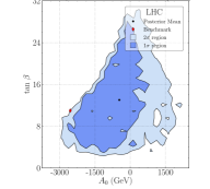
(a)

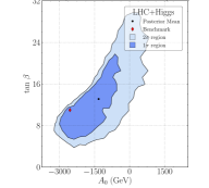
(b)

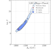
(c)

Figure 4: The $68\%$ (dark blue) and $95\%$ (light blue) credible regions of the $(A_{0},\,\tan\beta)$ plane of the CMSSM, adding the data one by one from left to right. The parameters $m_{1/2}$ and $m_{0}$ were marginalized. Our benchmark point is marked with a red diamond and the posterior mean is marked with a black circle. The bin limits are identical to the plot limits with $25$ bins per dimension.

The $(A_{0},\,\tan\beta)$ plane of the CMSSM in Fig. 4 tells a different story from that of the $(m_{0},\,m_{1/2})$ plane. With a likelihood from LHC in Fig. 4a, $(A_{0},\,\tan\beta)$ are poorly reconstructed; our credible regions exhibit a single, broad mode that omits the benchmark point. The unskewed shape of the credible regions indicate little correlation between $\tan\beta$ and $A_{0}$, though a slight positive correlation is visible. The reconstruction is significantly worse than for $(m_{0},\,m_{1/2})$, especially for $A_{0}$, which is determined to within $-3.5\,\text{TeV}\lesssim A_{0}\lesssim 1.5\,\text{TeV}$ at the $95\%$ level.

This is unsurprising. Because our LHC likelihood constrains only neutralino and first- and second-generation sparticle masses, at tree-level, it is independent of $A_{0}$ and dependent on $\tan\beta$ only in off-diagonal neutralino mass matrix elements from $F$-terms and diagonal sfermion mass matrix elements from $D$-terms. To first order, our credible regions on the $(A_{0},\,\tan\beta)$ plane with only LHC are determined by physicality conditions. Large $\tan\beta\gtrsim 30$ is excluded, because the stau is lighter than the neutralino. Similarly, large negative $A_{0}$ is disfavored at large $\tan\beta$, because in that corner of the $(A_{0},\,\tan\beta)$ plane off-diagonal trilinear and $F$-terms in sfermion mass matrices do not cancel.

Our credible regions, however, favor $A_{0}\lesssim 0$, similar to its benchmark, whereas physicality ought to marginally favor $A_{0}\gtrsim 0$. The preference for $A_{0}\lesssim 0$ stems from $\mu$ in the neutralino mass matrix. The wino-like, second-lightest neutralino’s mass is

$$m_{{\chi}^{0}_{2}}\approx M_{2}-\frac{M_{W}^{2}\left(M_{2}+\mu\sin 2\beta\right)}{\mu^{2}-M_{2}^{2}},$$ (22)

where $\mu$ is determined from the electroweak symmetry breaking condition. If $\mu$ decreases, the second-lightest neutralino’s higgsino component increases, and its mass decreases. The soft-breaking Higgs boson masses receive one-loop corrections proportional to the trilinear soft terms corresponding to the Yukawa couplings for the top and bottom quarks $|A_{t,b}|^{2}$, respectively, in their renormalization group equations from squark loop diagrams. Ultimately, $A_{0}$ affects $\mu$ via the renormalization group and an electroweak symmetry breaking condition, which affects neutralino masses. Thus, our LHC likelihood is somewhat sensitive to $A_{0}$.

Incidentally, there is no positive $A_{0}$ solution. Our benchmark has $A^{\text{BM}}_{t,b}\lesssim-2\,\text{TeV}$ at the electroweak scale. No equivalent solution with $|A^{\text{BM}}_{t,b}|$ exists. The $\beta$-functions for $A_{t,b}$ are negative and run quicker than that for $A_{\tau}$. For $|A^{\text{BM}}_{t,b}|$ at the electroweak scale, we would require $A_{0}\gtrsim 10\,\text{TeV}$. But such large $A_{0}$ is vetoed, because the stau is lighter than the neutralino.

The $(A_{0},\,\tan\beta)$ plane with only LHC requires $A_{0}\gtrsim-3\,\text{TeV}$ at the $95\%$ level. With larger negative $A_{0}$, the stau is the LSP, or, even if one simultaneously decreases $\tan\beta\lesssim 6$ to avoid stau LSP, the neutralino mass is already saturated at our benchmark. The correction in Eq. 22 is always negative. With our benchmark $A_{0}$, the correction is already approximately zero, because the neutralino is predominantly wino-like. With larger negative $A_{0}$, we cannot fine-tune the neutralino mass with $A_{0}$. In other words, because the second-lightest neutralino is entirely wino-like at our benchmark, one cannot decrease its higgsino component. With $A_{0}\gtrsim 0.5\,\text{TeV}$, with different corrections to bino- and wino-like neutralino masses, similar to the second term in Eq. 22, it becomes impossible to tune $(m_{0},\,m_{1/2})$ to maintain agreement with the pseudo-measurements.

Adding information from Higgs (Fig. 4b) helps somewhat improve reconstruction on the $(A_{0},\,\tan\beta)$ plane, with $A_{0}$ pushed down to negative values and $\tan\beta$ pushed to slightly higher values, without exceeding $\tan\beta\lesssim 30$ at $95\%$ established by LHC. The absolute value of $A_{0}$ is pushed heavier and $\tan\beta$ is pushed higher to tune stop-mixing so that $X_{t}/M_{\rm SUSY}\approx-\sqrt{6}$, which maximizes the Higgs boson mass, bringing it closer to its measured value.

Adding information from Planck (Fig. 4c) dramatically improves parameter reconstruction on the $(A_{0},\,\tan\beta)$ plane, though reveals strong positive correlation between $(A_{0},\,\tan\beta)$. The relic density is most sensitive in this region of the CMSSM to the stau mass, in contrast to our LHC likelihood, which is sensitive to only the first- and second-generation sleptons. Because the $\tau$ Yukawa coupling is significantly larger than the $e$ and $\mu$ Yukawa couplings, the stau is sensitive to mixing between left- and right-handed states, which splits the stau mass eigenvalues. This mixing is proportional to $X_{\tau}\equiv A_{\tau}-\mu\tan\beta$, and hence $m_{\tilde{\tau}_{1}}$ can be driven smaller so that is approximately mass degenerate with $m_{{\chi}^{0}_{1}}$ by increasing $\tan\beta$ or by increasing $|A_{\tau}|$. This enhances SC, thus decreasing the relic density to its measured Planck value. Because we require particular $X_{\tau}=\hat{X}_{\tau}\pm\Delta X_{\tau}$ to tune the lightest stau’s mass,

$$\hat{X}_{\tau}-\Delta X_{\tau} \lesssim A_{\tau}-\mu\tan\beta\lesssim\hat{X}_{\tau}+\Delta X_{\tau},$$ (23)

$$A_{\tau}-\hat{X}_{\tau}-\Delta X_{\tau} \lesssim\mu\tan\beta\lesssim A_{\tau}-\hat{X}_{\tau}+\Delta X_{\tau},$$

$\tan\beta$ must lie between close parallel lines on the $(A_{0},\,\tan\beta)$ plane, truncated at $A_{0}\sim 0$ and $A_{0}\sim-3\,\text{TeV}$ by limits established by our LHC and Higgs likelihoods in Fig. 4b.

Similarly to our statistics for $(m_{0},\,m_{1/2})$, our statistics for $A_{0}$ are biased, in that our distributions are not centered on our benchmark $A_{0}$. The cause is identical to that for $(m_{0},\,m_{1/2})$: decreases in $A_{0}$ from its benchmark result cannot increase the neutralino mass, because it is already saturated at our benchmark.

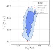
(a)

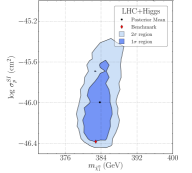
(b)

(c)

Figure 5: The $68\%$ (dark blue) and $95\%$ (light blue) credible regions of the $(m_{{\chi}^{0}_{1}},\,\sigma^{\rm SI}_{p})$ plane of the CMSSM, adding the data one by one from left to right. The posterior for these derived quantities was obtained by histogramming our samplesRuiz de Austri et al. (2006). Our benchmark point is marked with a red diamond and the posterior mean is marked with a black circle. The bin limits are identical to the plot limits with $25$ bins per dimension. The LUX limit (not shown) is $\sigma^{\rm SI}_{p}\lesssim 10^{-45}\,\text{cm}^{2}$.

We turn to the experimental quantities that would be of much interest in our scenario in which SUSY had been discovered. First, we consider DM direct detection experiments, which would attempt to verify SUSY as the DM. We plot credible regions on the $(m_{{\chi}^{0}_{1}},\,\sigma^{\rm SI}_{p})$ plane in Fig. 5. We found the posterior for these derived quantities by histogramming our samples weighted by the posteriorRuiz de Austri et al. (2006). The plot shows little correlation between $m_{{\chi}^{0}_{1}}$ and $\sigma^{\rm SI}_{p}$, and $m_{{\chi}^{0}_{1}}$ and $\sigma^{\rm SI}_{p}$ are both reasonably well-determined. Although $\sigma^{\rm SI}_{p}$ is determined at the $95\%$ level to within an order of magnitude, with only LHC, its distribution is biased towards $\sigma^{\rm SI}_{p}$ larger than its benchmark. The increasing $\sigma^{\rm SI}_{p}$ direction corresponds to the $m_{1/2}-m_{0}$ direction on the $(m_{0},\,m_{1/2})$ plane. As previously explained, the down-type higgsino component of the lightest neutralino increases along that direction on the $(m_{0},\,m_{1/2})$ plane and thus $\sigma^{\rm SI}_{p}$ increases.

The resolution and bias of $\sigma^{\rm SI}_{p}$ improves slightly as data is added, especially Planck, but the resolution of $m_{{\chi}^{0}_{1}}$ is not much improved by the additional information. Nevertheless, the precision of the CMSSM direct detection predictions indicate that in our discovery scenario we would know that DM might be within reach of direct detection experiments in the foreseeable future and be able to decide which experiments to build accordingly. Our scenario might be inaccessible at LUX and Xenon100, but should be accessible at a 1-tonne detectors whose reach is expected to be below $10^{-46}\,\text{cm}^{2}$ in the neutralino mass range typical for our benchmark point. On the other hand, prospects for current or future gamma-ray experiments, like CTA, look hopelessRoszkowski et al. (2014a, b).

Finally, we consider the rare decay $\textrm{BR}\left(B_{s}\to\mu^{+}\mu^{-}\right)$, which, if it deviates from its SM value, could indicate the presence of new physics. LHCbAaij et al. (2013) and CMSChatrchyan et al. (2013b), recently measured $\textrm{BR}\left(B_{s}\to\mu^{+}\mu^{-}\right)$ with statistical significance but limited precision as $\textrm{BR}\left(B_{s}\to\mu^{+}\mu^{-}\right)=3.1\pm 0.7\times 10^{-9}$Beringer et al. (2012). We found that in our scenario one could make a CMSSM prediction for $\textrm{BR}\left(B_{s}\to\mu^{+}\mu^{-}\right)$ that agreed with the SM prediction within a $\sim 10\%$ uncertainty, stemming from uncertainties in the sparticle mass spectrum and parametric uncertainties in SM nuisance parameters. Unfortunately, it probably would not provide a channel for independently verifying our benchmark point.

VI Conclusions

Assuming that the CMSSM is a viable model, we identified a benchmark point in the CMSSM’s heavy SC region that is in agreement with experimental constraints. We demonstrated that our benchmark could be discovered at the LHC at $\sqrt{s}={14}\,\text{TeV}$ with $300/\text{fb}$ via the golden decay, in which a squark decays via a slepton to opposite-sign-same-flavor leptons, a jet and missing energy. We simulated invariant mass distributions from this decay in Monte-Carlo. From kinematic endpoints in these distributions, we showed that we could measure the masses of two lightest neutralinos, a squark and a slepton, with a methodology identical to that in preliminary LHC studies. We found that these measurements were quite precise, with small, correlated errors, described by our covariance matrix.

We investigated, with Bayesian statistics, whether in our benchmark scenario we could determine the CMSSM’s Lagrangian parameters from the sparticle mass measurements. CMSSM parameters can be accurately determined; our Bayesian credible regions enveloped the benchmark parameters, though $A_{0}$ was recovered with limited precision, and the credible regions indicated bias. To investigate the impact of Higgs boson mass and relic density measurements, we added likelihoods describing these measurements, and repeated our Bayesian analysis. We found that the additional experiments had limited impact, though helped to determine $A_{0}$. Lastly, we considered whether, in our benchmark scenario, we could make precise predictions for experimental observables, with which one could verify that the kinematic endpoints were from the CMSSM, and that the CMSSM’s neutralino was dark matter. We found that the spin-independent proton scattering cross section, relevant to the direct detection of dark matter, could be predicted to within an order of magnitude and will be accessible to oncoming one tonne detectors. A prediction for the branching ratio for the rare decay $B_{s}\to\mu^{+}\mu^{-}$, however, with heavier, approximately decoupled sparticles and small $\tan\beta$, was limited by parametric errors from SM nuisance parameters and errors in the CMSSM’s Lagrangian parameters.