On the role of a priori knowledge in the optimization of quantum information processing

Abstract

This paper explores the role of a priori knowledge in the optimization of quantum information processing by investigating optimum unambiguous discrimination problems for both the qubit and qutrit states. In general, a priori knowledge in optimum unambiguous discrimination problems can be classed into two types: a priori knowledge of discriminated states themselves and a priori probabilities of preparing the states. It is clarified that whether a priori probabilities of preparing discriminated states are available or not, what type of discriminators one should design just depends on what kind of the classical knowledge of discriminated states. This is in contrast to the observation that choosing the parameters of discriminators not only relies on the a priori knowledge of discriminated states, but also depends on a priori probabilities of preparing the states. Two types of a priori knowledge can be utilized to improve optimum performance but play the different roles in the optimization from the view point of decision theory.

1 Introduction

Based on the observation that information is represented, stored, processed, transmitted and readout by physical systems, Rolf Landauer famously remarked that information is physical. Until recently, information was largely thought of in classical terms with quantum mechanics playing at most a supportive role in designing the equipment to store and process information. However, technological advances have ensured that quantum effects play an increasingly important role. This has motivated the birth of quantum information theory q1 , which is currently attracting enormous interest due to its fundamental nature and potentially important applications in quantum teleportationR1 ; R2 , dense codingR4 , quantum cryptographyR5 ; R6 ; R7 , and quantum computation c1 ; c2 ; c6 .

Quantum information theory can be considered as an extension and generalization of classical information theoryqc2 but there are many important and special problems in this domain. One of these is the role of a priori knowledge in quantum information processing. Researchers have explored numerous ways to develop programmable quantum devices 5 to accomplish various quantum information processing tasks such as storing quantum dynamics in quantum states8 , implementation of quantum maps9 , evaluating the expectation value of any operator11 and quantum state discrimination12 ; 13 ; 14 ; 15 ; 16 . These methods are based on the full utilization of a priori knowledge. However, the role of a priori knowledge in quantum information processing has not been fully explored so far, and this problem deserves the further investigation.

How to make optimal decisions based on full utilization of a priori knowledge is an important issue in various domains, especially in classical statistical decision theory decision . To address the problem of the use of a priori knowledge in quantum information, we have to start with two basic questions: what does a priori knowledge mean in this domain and what role does a priori knowledge play in the optimization of quantum information processing? Since quantum state discrimination 4 ; A1 ; A2 ; A3 is very fundamental in the domain of quantum information processing3 , it is reasonable to carefully explore optimum unambiguous discrimination problems given various types of a priori knowledge.

In general, there are two types of a priori knowledge in optimum unambiguous discrimination problems: a priori knowledge of discriminated states themselves (a priori knowledge of Type I) and a priori probabilities of preparing these states (a priori knowledge of Type II). Type-I knowledge can be expressed in a variety of forms. Even when the discriminated states are classically unknown, a single copy of them can be considered as a special form of a priori knowledge. By making full use of a single copy of the classically unknown states, Bergou and Hillery 12 constructed an unambiguous discriminator, and Bergou et.al 16 showed how to construct devices that can optimally discriminate between a classically known and a classically unknown state. Recently qic , the effect of complete or incomplete a priori classical knowledge of discriminated states on the optimum unambiguous discrimination has been investigated when a priori probabilities of preparing the discriminated states are known.

Under different conditions of a priori knowledge, optimum unambiguous discrimination problems are reduced to different optimization problems. What kind of optimization problems can optimum unambiguous discrimination problems be reduced to? This depends on a priori knowledge of both Type I and Type II. A priori probabilities of preparing discriminated states are presumed known in many research papers 12 ; 15 ; 16 although optimal measurement for quantum-state discrimination without a priori probabilities has also been considered ad . However, optimum unambiguous discrimination problems have not been thoroughly investigated under various types of a priori knowledge so far. Specially, the optimum unambiguous discrimination problems have not been explored for multi-level quantum states under different a priori conditions. Therefore, we would like to exploit the role of a priori knowledge in the optimization by considering the optimum unambiguous discrimination problems for both the qubit and qutrit states in this paper. In this paper, the effect of a priori knowledge of both Type I and Type II on the optimization will be examined carefully for both the qubit states and qutrit states. We will show how to design discriminators that depend only on whether the classical knowledge of the discriminated states is complete or incomplete. How to choose the parameters of the discriminators, however, relies on a priori knowledge of both Type I and Type II.

The rest of this paper is organized as follows. In Sect. II, we comprehensively present the results on optimal unambiguous discrimination problems for two qubit states with and without different a priori preparing probability of the qubit states. The comparative analysis and some further discussions are present for optimal unambiguous discrimination problems of two qubit states in Sect. III. To further clarify the role of a priori information in the optimal decision and optimum success probability, we study the optimal unambiguous discrimination for two qutrit states in Sect. IV. The paper concludes with Sect. V.

2 Optimal unambiguous discrimination problems for two qubit states

To analysis the effect of a priori information of the discriminated states on optimum unambiguous discriminators and optimum success probabilities of unambiguously discriminating two qubit states, we review the results on optimal unambiguous discrimination problems with the knowledge of a priori preparing probabilities in the first three subsections. According to what kind of classical knowledge can be utilized, the 4 cases are discussed in the three subsections.

Case A1, without classical knowledge of either state but with a single copy of unknown states;

Case A2, with only classical knowledge of one of the two states and a single copy of the other unknown state;

Case A3, with only classical knowledge of one of the two states and the absolute value of the inner product of both states, and also with a single copy of the other unknown state;

Case A4, with classical knowledge of both states.

The A1 and A4 cases will be investigated in subsection A and C, respectively, and the A2 and A3 cases will be studied in subsection B.

Since a priori probabilities of preparing discriminated states are often presumed known, optimal unambiguous discrimination problems without a priori preparing probability may be skipped to a certain degree, and have not been thoroughly investigated so far. In the subsections D, E and F, we will further discuss various optimal unambiguous discrimination problems without a priori preparing probability. We have also four cases taken into consideration as follow.

Case B1, without classical knowledge of either state but with a single copy of unknown states;

Case B2, with classical knowledge of one of the two states and a single copy of the other unknown state;

Case B3, with classical knowledge of one of the two states and the absolute value of the inner product of both states, and also with a single copy of the other unknown state;

Case B4, with classical knowledge of both states.

The B1 and B4 cases will be investigated in subsection D and F, respectively, and the B2 and B3 cases will be studied in subsection E.

2.1 Optimal unambiguous discrimination problems for Case A1

In this subsection, we review the result of Ref. 12 , and further discuss the optimal unambiguous discrimination problems in which the preparing probabilities is given, but none classical knowledge of discriminated states is available.

Given two unknown quantum states $|\psi_{1}\rangle$ and $|\psi_{2}\rangle$, we can construct a device to unambiguously discriminate between them. Two classically unknown states $|\psi_{1}\rangle$ and $|\psi_{2}\rangle$ are provided as two inputs for two program registers, respectively. Then we are given another qubit that is guaranteed to be one of two unknown states $|\psi_{1}\rangle$ and $|\psi_{2}\rangle$ stored in the two program registers. Our task is to determine, as best we can, which one the given qubit is. We are allowed to fail, but not to make a mistake. What is the best procedure to accomplish this? Our task is then reduced to the following measurement optimization problem.

One has two input states

$$|\Psi_{1}^{in}\rangle=|\psi_{1}\rangle_{A}|\psi_{1}\rangle_{B}|\psi_{2}\rangle_{C}$$ (1)

and

$$|\Psi_{2}^{in}\rangle=|\psi_{1}\rangle_{A}|\psi_{2}\rangle_{B}|\psi_{2}\rangle_{C}$$ (2)

where the subscripts $A$ and $C$ refer to the program registers, and the subscript $B$ refers to the data register. Our goal is to unambiguously distinguish between these inputs.

Let the elements of our POVM (positive-operator-valued measure) be $\Pi_{1}$, corresponding to unambiguously detecting $|\psi_{1}\rangle$, $\Pi_{2}$, corresponding to unambiguously detecting $|\psi_{2}\rangle$, and $\Pi_{0}$, corresponding to failure, respectively. The probabilities of successfully identifying the two possible input states are given by

$$\langle\Psi_{1}^{in}|{\Pi}_{1}|\Psi_{1}^{in}\rangle=p_{1}$$ (3)

and

$$\langle\Psi_{2}^{in}|{\Pi}_{2}|\Psi_{2}^{in}\rangle=p_{2}$$ (4)

and the condition of no errors implies that

$${\Pi}_{1}|\Psi_{2}^{in}\rangle=0;\ {\Pi}_{2}|\Psi_{1}^{in}\rangle=0$$ (5)

In addition, because the alternatives represented by the POVM exhaust all possibilities, we have that

$${\Pi}_{1}+{\Pi}_{2}+{\Pi}_{0}=I$$ (6)

Since we have no classical knowledge about $|\psi_{1}\rangle$ and $|\psi_{2}\rangle$, the right way of constructing POVM operators is to take advantage of the symmetrical properties of the states. Denoting $|0\rangle$ and $|1\rangle$ as two vectors of a basis, we define the antisymmetric state

$$|\psi_{BC}^{-}\rangle=\frac{1}{\sqrt{2}}(|0\rangle_{B}|1\rangle_{C}-|1\rangle_{B}|0\rangle_{C})$$ (7)

and

$$|\psi_{AB}^{-}\rangle=\frac{1}{\sqrt{2}}(|0\rangle_{A}|1\rangle_{B}-|1\rangle_{A}|0\rangle_{B})$$ (8)

and introduce the projectors to the antisymmetric subspaces of the corresponding qubit as

$$P_{BC}^{as}=|\psi_{BC}^{-}\rangle\langle\psi_{BC}^{-}|$$ (9)

and

$${P}_{AB}^{as}=|\psi_{AB}^{-}\rangle\langle\psi_{AB}^{-}|$$ (10)

We now can take for ${\Pi}_{1}$ and ${\Pi}_{2}$ operators

$${\Pi}_{1}=\lambda_{1}I_{A}\otimes{P}_{BC}^{as}$$ (11)

and

$${\Pi}_{2}=\lambda_{2}{P}_{AB}^{as}\otimes{I_{C}}$$ (12)

To assure that ${\Pi}_{1}$, ${\Pi}_{2}$ and ${\Pi}_{0}=I-{\Pi}_{1}-{\Pi}_{2}$ be semi-positive operators, the following constraints should be satisfied:

$$2-\lambda_{1}-\lambda_{2}\geq 0;\ 1-\lambda_{1}-\lambda_{2}+\frac{3}{4}\lambda_{1}\lambda_{2}\geq 0$$ (13)

After some calculations, we have $p_{i}=\frac{1}{2}\lambda_{i}(1-{\beta}^{2})$, where $i=1,2$ and $\beta=|\langle\psi_{1}|\psi_{2}\rangle|$. Suppose that $\eta_{1}$ is the preparation probability of $|\psi_{1}\rangle$, the average success probability is $P=p_{1}\eta_{1}+p_{2}(1-\eta_{1})$.

Since we have knowledge of $\eta_{1}$, our task is reduced to designing $\lambda_{1}(\eta_{1})$ and $\lambda_{2}(\eta_{1})$ such that the following average success probability

$$P={\frac{1}{2}[\lambda_{1}\eta_{1}+\lambda_{2}(1-\eta_{1})](1-{\beta}^{2})}$$ (14)

is maximal with the constrains given by Eq. (13). This is to say, the loss function can be expressed as

$$J=\max\min_{\{\eta_{1}\}}\{{\frac{1}{2}[\lambda_{1}\eta_{1}+\lambda_{2}(1-\eta_{1})](1-{\beta}^{2})}\}$$ (15)

In this case, the optimum success probability has been summarized as follows

$$P_{0}^{opt}(\beta,\eta_{1})=\ \bigg{\{}\begin{array}[]{cc}\frac{1}{2}(1-\eta_{1})(1-{\beta}^{2})&\eta_{1}\leq{\frac{1}{5}}\\ \frac{2}{3}[1-\sqrt{\eta_{1}(1-\eta_{1})}](1-{\beta}^{2})&\frac{1}{5}\leq{\eta_{1}}\leq{\frac{4}{5}}\\ \frac{1}{2}\eta_{1}(1-{\beta}^{2})&\eta_{1}\geq{\frac{4}{5}}\end{array}$$ (16)

where the subscript $0$ of $P_{0}^{opt}$ means that we have no a priori classical knowledge of $|\psi_{1}\rangle$ and $|\psi_{2}\rangle$ and the corresponding optimal action parameters are given by

$$\lambda_{1}^{0,opt}(\eta_{1})=\ \bigg{\{}\begin{array}[]{cc}0&\eta_{1}\leq{\frac{1}{5}}\\ \frac{2}{3}[2-\sqrt{\frac{1-\eta_{1}}{\eta_{1}}}]&\frac{1}{5}\leq{\eta_{1}}\leq{\frac{4}{5}}\\ 1&\eta_{1}\geq{\frac{4}{5}}\end{array}$$ (17)

and

$$\lambda_{2}^{0,opt}(\eta_{1})=\ \bigg{\{}\begin{array}[]{cc}1&\eta_{1}\leq{\frac{1}{5}}\\ \frac{2}{3}[2-\sqrt{\frac{\eta_{1}}{1-\eta_{1}}}]&\frac{1}{5}\leq{\eta_{1}}\leq{\frac{4}{5}}\\ 0&\eta_{1}\geq{\frac{4}{5}}\end{array}$$ (18)

Remark: We would like to underline that the we make the optimal decision in Eqs. (17) and (18) without the knowledge $\beta$, but the optimum success probability (16) is the function of both $\beta$ and $\eta_{1}$.

2.2 Optimal unambiguous discrimination problems for Cases A2 and A3

In this subsection, we re-discuss the optimal unambiguous discrimination problem for the cases A2 and A3 from the view point of decision theory, and throw some new insights, which are different from those in Ref. 16 ; qic .

Given one known quantum state $|\psi_{1}\rangle$ and one unknown quantum state $|\psi_{2}\rangle$, we can construct a device that unambiguously discriminate between them. We shall consider the following problem which may be a simple version of a programmable state discriminator. The unknown state $|\psi_{2}\rangle$ is provided as an input for the program register. Then we are given another qubit that is guaranteed to be in the known state $|\psi_{1}\rangle$ or the unknown state $|\psi_{2}\rangle$ stored in the program register. Our task is to determine, as best we can, which one the given qubit is. As in case A1, we are allowed to fail, but not to make a mistake. What is the best procedure to accomplish this?

In line with Ref. 12 , one can construct such a device by viewing this problem as a task in measurement optimization. The measurement is allowed to return an inconclusive result but never an erroneous one. Thus, it will be described by a POVM that will return outcome $1$ (the unknown state stored in the data register matches the known state $|\psi_{1}\rangle$), $2$ (the unknown state stored in the data register matches $|\psi_{2}\rangle$ in the program register), or $0$ (we do not learn anything about the unknown state stored in the data register). Our task is then reduced to the following measurement optimization problem.

One has two input states

$$|\Psi_{1}^{in}\rangle=|\psi_{2}\rangle_{A}|\psi_{1}\rangle_{B}$$ (19)

and

$$|\Psi_{2}^{in}\rangle=|\psi_{2}\rangle_{A}|\psi_{2}\rangle_{B}$$ (20)

where the subscript $A$ refers to the program register ($A$ contains $|\psi_{2}\rangle$), and the subscript $B$ refers to the data register. Our goal is to unambiguously distinguish between these inputs.

Let the elements of our POVM be $\Pi_{1}$, corresponding to unambiguously detecting $|\psi_{1}\rangle$, $\Pi_{2}$, corresponding to unambiguously detecting $|\psi_{2}\rangle$, and $\Pi_{0}$, corresponding to failure, respectively. The probabilities of successfully identifying the two possible input states are given by

$$\langle\Psi_{1}^{in}|{\Pi}_{1}|\Psi_{1}^{in}\rangle=p_{1}$$ (21)

and

$$\langle\Psi_{2}^{in}|{\Pi}_{2}|\Psi_{2}^{in}\rangle=p_{2}$$ (22)

and the condition of no errors implies that

$${\Pi}_{1}|\Psi_{2}^{in}\rangle=0;\ {\Pi}_{2}|\Psi_{1}^{in}\rangle=0$$ (23)

In addition, because the alternatives represented by the POVM exhaust all possibilities, we have that

$${\Pi}_{1}+{\Pi}_{2}+{\Pi}_{0}=I$$ (24)

Since we know nothing about $|\psi_{2}\rangle$ but have the classical knowledge of $|\psi_{1}\rangle$, the right way of constructing POVM operators is to take advantage of the symmetrical properties of the state as well as the classical knowledge of $|\psi_{1}\rangle$. Denoting $|\psi_{1}^{\perp}\rangle$ as the unit vector orthogonal to $|\psi_{1}\rangle$, we define the antisymmetric state

$$|\psi_{AB}^{-}\rangle=\frac{1}{\sqrt{2}}(|\psi_{1}\rangle_{A}|\psi_{1}^{\perp}\rangle_{B}-|\psi_{1}^{\perp}\rangle_{A}|\psi_{1}\rangle_{B})$$ (25)

and introduce the projectors to the antisymmetric subspaces of the corresponding qubit as

$${P}_{AB}^{as}=|\psi_{AB}^{-}\rangle\langle\psi_{AB}^{-}|$$ (26)

Remark: suppose $|\psi_{1}\rangle$ can be expressed in terms of a basis of $|0\rangle$ and $|1\rangle$ as $|\psi_{1}\rangle=\cos\frac{\theta}{2}|0\rangle+e^{i\phi}\sin\frac{\theta}{2}|1\rangle$ where $0\leq\phi<2\pi$ and $0\leq\theta\leq\pi$, then we can choose $|\psi_{1}^{\perp}\rangle=\sin\frac{\theta}{2}|0\rangle-e^{i\phi}\cos\frac{\theta}{2}|1\rangle$.

By making full use of the knowledge of $|\psi_{1}\rangle$ and $|\psi_{1}^{\perp}\rangle$, we construct the measurement operators ${\Pi}_{1}$ and ${\Pi}_{2}$ to satisfy the no-error condition given by Eq.(23) as follows:

$${\Pi}_{1}=\lambda_{1}{P}_{AB}^{as}$$ (27)

and

$${\Pi}_{2}=\lambda_{2}{|\psi_{1}\rangle_{A}|\psi_{1}^{\perp}\rangle_{B}{{}_{B}\langle}\psi_{1}^{\perp}|_{A}\langle\psi_{1}|}+\lambda_{3}{|\psi_{1}^{\perp}\rangle_{A}|\psi_{1}^{\perp}\rangle_{B}{{}_{B}\langle}\psi_{1}^{\perp}|_{A}\langle\psi_{1}^{\perp}|}$$ (28)

where $\lambda_{1}$, $\lambda_{2}$ and $\lambda_{3}$ are undetermined nonnegative real numbers. Using the Eqs. (27) and (28), we have

$$p_{1}=\langle\Psi_{1}^{in}|{\Pi}_{1}|\Psi_{1}^{in}\rangle=\frac{1}{2}\lambda_{1}(1-\beta^{2})$$ (29)

$$p_{2}=\langle\Psi_{2}^{in}|{\Pi}_{2}|\Psi_{2}^{in}\rangle=\lambda_{2}\beta^{2}(1-\beta^{2})+\lambda_{3}(1-\beta^{2})^{2}$$ (30)

By assuming that the preparation probabilities of $|\psi_{1}\rangle$ and $|\psi_{2}\rangle$ are $\eta_{1}$ and $\eta_{2}$ (where $\eta_{2}=1-\eta_{1}$), respectively, we can define the average probability $P$ of successfully discriminating two states as

$$P=[\frac{1}{2}\lambda_{1}\eta_{1}+\lambda_{2}\beta^{2}\eta_{2}+\lambda_{3}(1-\beta^{2})\eta_{2}](1-\beta^{2})$$ (31)

where $\beta=|\langle\psi_{1}|\psi_{2}\rangle|$, and our task is to maximize the performance Eq. (31) subject to the constraint that ${\Pi}_{0}=I-{\Pi}_{1}-{\Pi}_{2}$ is a positive operator.

To assure that ${\Pi}_{0}$, ${\Pi}_{1}$ and ${\Pi}_{2}$ are positive operators, we have the following inequality constraints:

$$1-{\lambda_{1}}-{\lambda_{2}}+\frac{1}{2}{\lambda_{1}}{\lambda_{2}}\geq 0$$ (32)

and

$$0\leq{\lambda_{i}}\leq 1(i=1,2,3)$$ (33)

Subsequently, we will discuss our strategies for the A2 and A3 cases.

(i) For the A2 case, we have the knowledge of preparing probability $\eta_{1}$, but no knowledge of $\beta$. It can be demonstrated that one cannot maximize Eq. (31) everywhere simultaneously without the classical knowledge of $\beta$. Still, we can give some further analysis.

Our strategy is to design $\lambda^{1,w\beta}_{1}(\eta)$, $\lambda^{1,w\beta}_{2}(\eta)$ and $\lambda^{1,w\beta}_{3}(\eta)$ to optimize the performance

$$J=\max\min_{\{\beta\}}[\frac{1}{2}\lambda_{1}\eta_{1}+\lambda_{2}(1-\eta_{1})+(\lambda_{3}-\lambda_{2})(1-\beta^{2})(1-\eta_{1})]$$ (34)

subject to the constraints described by Eqs. (32) and (33).

No matter what $\eta_{1}$ is, one should always choose $\lambda^{1,w\beta}_{3}(\eta_{1})=1$. As for $\lambda^{1,w\beta}_{1}(\eta_{1})$ and $\lambda^{1,w\beta}_{2}(\eta_{1})$, the problem is reduced to maximizing $\frac{1}{2}\lambda_{1}\eta_{1}+\lambda_{2}(1-\eta_{1})$ subject to the constraints described by Eqs. (32) and (33).

After some calculations, we have

$$\lambda_{1}^{1,w\beta}(\eta_{1})=\ \bigg{\{}\begin{array}[]{cc}0&\eta_{1}\leq{\frac{1}{2}}\\ 2(1-\sqrt{\frac{1-\eta_{1}}{\eta_{1}}})&\frac{1}{2}\leq{\eta_{1}}\leq{\frac{4}{5}}\\ 1&\eta_{1}\geq{\frac{4}{5}}\end{array}$$ (35)

and

$$\lambda_{2}^{1,w\beta}(\eta_{1})=\ \bigg{\{}\begin{array}[]{cc}1&\eta_{1}\leq{\frac{1}{2}}\\ 2-\sqrt{\frac{\eta_{1}}{1-\eta_{1}}}&\frac{1}{2}\leq{\eta_{1}}\leq{\frac{4}{5}}\\ 0&\eta_{1}\geq{\frac{4}{5}}\end{array}$$ (36)

and

$$\lambda^{1,w\beta}_{3}(\eta_{1})=1$$ (37)

By substituting $\lambda^{1,w\beta}_{1}(\eta_{1})$, $\lambda^{{1,w\beta}}_{2}(\eta_{1})$ and $\lambda^{1,{w\beta}}_{3}(\eta_{1})$ into (31), we obtain the actual optimum success probability in this strategy:

$$P_{1}^{w\beta}(\beta,\eta_{1})=\ \bigg{\{}\begin{array}[]{cc}P_{1_{1}}^{w\beta}(\beta,\eta_{1})&\eta_{1}\leq{\frac{1}{2}}\\ P_{1_{2}}^{w\beta}(\beta,\eta_{1})&\frac{1}{2}\leq{\eta_{1}}\leq{\frac{4}{5}}\\ P_{1_{3}}^{w\beta}(\beta,\eta_{1})&\eta_{1}\geq{\frac{4}{5}}\end{array}$$ (38)

with

$$P_{1_{1}}^{w\beta}(\beta,\eta_{1})=(1-\eta_{1})(1-{\beta}^{2})$$ (39)

and

$$P_{1_{2}}^{w\beta}(\beta,\eta_{1})=[1+{\beta}^{2}(1-\eta_{1})-(1+{\beta}^{2})\sqrt{\eta_{1}(1-\eta_{1})}](1-{\beta}^{2})$$ (40)

and

$$P_{1_{3}}^{w\beta}(\beta,\eta_{1})=[1-\frac{1}{2}\eta_{1}-{\beta}^{2}(1-\eta_{1})](1-{\beta}^{2})$$ (41)

where the subscript $1$ of $P_{1}^{w\beta}$ means that we just have a priori classical knowledge of $|\psi_{1}\rangle$, one of two discriminated states, and the superscript $w\beta$ of $P_{1}^{w\beta}$ implies that the actual optimum success probability is obtain for the worst case of $\beta$.

Remark: In this case, our “optimal” actions or decisions in Eqs. (35-37) can be only considered as the function of the preparing probability $\eta_{1}$ but the actual success probability given by Eq. (38) with Eqs. (39-41) is still the function of both $\beta$ and $\eta_{1}$ even when we have no idea about $\beta$.

(ii) With a priori classical knowledge of both $|\langle\psi_{1}|\psi_{2}\rangle|=\beta$ and $\eta_{1}$ in hand, our task in the third case is to get the optimum values $\lambda^{1+,opt}_{1}(\beta,\eta_{1})$, $\lambda^{1+,opt}_{2}(\beta,\eta_{1})$ and $\lambda^{1+,opt}_{3}(\beta,\eta_{1})$ to optimize the average success probability

$$J=[\frac{1}{2}\lambda_{1}\eta_{1}+\lambda_{2}\beta^{2}(1-\eta_{1})+\lambda_{3}(1-\beta^{2})(1-\eta_{1})](1-\beta^{2})$$ (42)

subject to the constraints Eqs. (32) and (33).

After some calculations, we have

$$\lambda^{1+,opt}_{1}(\beta,\eta_{1})=\ \bigg{\{}\begin{array}[]{cc}0&\eta_{1}\leq\frac{{\beta}^{2}}{1+{\beta}^{2}}\\ 2(1-\beta\sqrt{\frac{1-\eta_{1}}{\eta_{1}}})&\frac{{\beta}^{2}}{1+{\beta}^{2}}\leq{\eta_{1}}\leq{\frac{4{\beta}^{2}}{1+4{\beta}^{2}}}\\ 1&\eta_{1}\geq{{\frac{4{\beta}^{2}}{1+4{\beta}^{2}}}}\end{array}$$ (43)

and

$$\lambda^{1+,opt}_{2}(\beta,\eta_{1})=\ \bigg{\{}\begin{array}[]{cc}1&\eta_{1}\leq\frac{{\beta}^{2}}{1+{\beta}^{2}}\\ 2-\frac{1}{\beta}\sqrt{\frac{\eta_{1}}{1-\eta_{1}}}&\frac{{\beta}^{2}}{1+{\beta}^{2}}\leq{\eta_{1}}\leq{\frac{4{\beta}^{2}}{1+4{\beta}^{2}}}\\ 0&\eta_{1}\geq{{\frac{4{\beta}^{2}}{1+4{\beta}^{2}}}}\end{array}$$ (44)

and

$$\lambda^{1+,opt}_{3}(\beta,\eta_{1})\equiv 1$$ (45)

Taking Eq. (42) into consideration, we obtain the corresponding optimum success probabilities:

$$P_{1+}^{opt}(\beta,\eta_{1})=\ \bigg{\{}\begin{array}[]{cc}P_{1+_{1}}^{opt}(\beta,\eta_{1})&\eta_{1}\leq\frac{{\beta}^{2}}{1+{\beta}^{2}}\\ P_{1+_{2}}^{opt}(\beta,\eta_{1})&\frac{{\beta}^{2}}{1+{\beta}^{2}}\leq{\eta_{1}}\leq{\frac{4{\beta}^{2}}{1+4{\beta}^{2}}}\\ P_{1+_{3}}^{opt}(\beta,\eta_{1})&\eta_{1}\geq{{\frac{4{\beta}^{2}}{1+4{\beta}^{2}}}}\end{array}$$ (46)

with

$$P_{1+_{1}}^{opt}(\beta,\eta_{1})=(1-\eta_{1})(1-\beta^{2})$$ (47)

and

$$P_{1+_{2}}^{opt}(\beta,\eta_{1})=[1+{\beta}^{2}(1-\eta_{1})-2\beta\sqrt{\eta_{1}(1-\eta_{1})}](1-\beta^{2})$$ (48)

and

$$P_{1+_{3}}^{opt}(\beta,\eta_{1})=[1-\frac{1}{2}\eta_{1}-\beta^{2}(1-\eta_{1})](1-\beta^{2})$$ (49)

where the subscript $1+$ of $P_{1+}^{opt}$ means that we have a priori classical knowledge of one of the two discriminated states and the absolute value of the inner product of the two states.

Remark: In the Case A3, both the optimal actions or decisions in Eqs. (43-45) and the actual success probability given by Eq. (46) with Eqs. (47-49) can be considered as the functions of both $\beta$ and $\eta_{1}$.

2.3 Optimal unambiguous discrimination problems for A4

In this subsection, we recall the result of Ref. 3 ; A4 for the A4 case.

If we have complete a priori classical knowledge of both $|\psi_{1}\rangle$ and $|\psi_{2}\rangle$, the measurement is performed on the detected qubit. One can select the detection operators as

$${\Pi}_{1}=\lambda_{1}{|\psi_{2}^{\perp}\rangle\langle\psi_{2}^{\perp}|}$$ (50)

and

$${\Pi}_{2}=\lambda_{2}{|\psi_{1}^{\perp}\rangle\langle\psi_{1}^{\perp}|}$$ (51)

Our task is to choose $\lambda_{1}$ and $\lambda_{2}$ based on a priori information such that the average success probability

$$P=[\lambda_{1}\eta_{1}+\lambda_{2}(1-\eta_{1})](1-\beta^{2})$$ (52)

is maximized. This is to say, the loss function can be expressed as

$$J=\max\min_{\{\eta_{1}\}}\{{\frac{1}{2}[\lambda_{1}\eta_{1}+\lambda_{2}(1-\eta_{1})](1-{\beta}^{2})}\}$$ (53)

To assure that ${\Pi}_{0}$, ${\Pi}_{1}$ and ${\Pi}_{2}$ are positive operators, we have the following inequality constraints:

$$1-\lambda_{1}-\lambda_{2}\beta^{2}\geq 0$$ (54)

and

$$1-\lambda_{1}-\lambda_{2}+(1-\beta^{2})\lambda_{1}\lambda_{2}\geq 0$$ (55)

where $|\langle\psi_{1}|\psi_{2}\rangle|=\beta$.

Since we have knowledge of preparing probability $\eta_{1}$ and $\beta$, we will make the following decision

$$\lambda_{1}^{2,opt}(\beta,\eta_{1})=\ \bigg{\{}\begin{array}[]{cc}0&\eta_{1}\leq{\frac{\beta^{2}}{1+\beta^{2}}}\\ \frac{1}{1-\beta^{2}}(1-\beta\sqrt{\frac{1-\eta_{1}}{\eta_{1}}})&\frac{\beta^{2}}{1+\beta^{2}}\leq{\eta_{1}}\leq{\frac{1}{1+\beta^{2}}}\\ 1&\eta_{1}\geq{\frac{1}{1+\beta^{2}}}\end{array}$$ (56)

and

$$\lambda_{2}^{2,opt}(\beta,\eta_{1})=\ \bigg{\{}\begin{array}[]{cc}1&\eta_{1}\leq{\frac{\beta^{2}}{1+\beta^{2}}}\\ \frac{1}{1-\beta^{2}}(1-\beta\sqrt{\frac{\eta_{1}}{1-\eta_{1}}})&\frac{\beta^{2}}{1+\beta^{2}}\leq{\eta_{1}}\leq{\frac{1}{1+\beta^{2}}}\\ 0&\eta_{1}\geq{\frac{1}{1+\beta^{2}}}\end{array}$$ (57)

Furthermore, we can obtain the optimum success probability for this case (also as per Ref. 3 ; A4 ).

$$P_{2}^{opt}(\beta,\eta_{1})=\ \bigg{\{}\begin{array}[]{cc}P_{2_{1}}^{opt}(\beta,\eta_{1})&\eta_{1}\leq{\frac{\beta^{2}}{1+\beta^{2}}}\\ P_{2_{2}}^{opt}(\beta,\eta_{1})&\frac{\beta^{2}}{1+\beta^{2}}\leq{\eta_{1}}\leq{\frac{1}{1+\beta^{2}}}\\ P_{2_{3}}^{opt}(\beta,\eta_{1})&\eta_{1}\geq{\frac{1}{1+\beta^{2}}}\end{array}$$ (58)

with

$$P_{2_{1}}^{opt}(\beta,\eta_{1})=(1-\eta_{1})(1-\beta^{2})$$ (59)

and

$$P_{2_{2}}^{opt}(\beta,\eta_{1})=1-2\sqrt{\eta_{1}(1-\eta_{1})}\beta$$ (60)

and

$$P_{2_{3}}^{opt}(\beta,\eta_{1})=\eta_{1}(1-\beta^{2})$$ (61)

where $|\langle\psi_{1}|\psi_{2}\rangle|=\beta$, the subscript $2$ of $P_{2}^{opt}$ means that we have the classical knowledge of both discriminated states.

Remark: For the Case A4, it is not surprising to find that the optimal actions or decisions in Eqs. (56-57) and the optimal success probability given by Eq. (58) with Eqs. (59-61) are the function of both $\beta$ and $\eta_{1}$.

2.4 Optimal unambiguous discrimination problems for Case B1

Since we have the same classical knowledge of discriminated states in this case as in Section II. A, we can follow the analysis in Section II. A and choose ${\Pi}_{1}$ and ${\Pi}_{2}$ as Eqs. (11) and (12).

To assure that ${\Pi}_{1}$, ${\Pi}_{2}$ and ${\Pi}_{0}=I-{\Pi}_{1}-{\Pi}_{2}$ be semi-positive operators, the constraints on $\lambda_{1}$ and $\lambda_{2}$ described by Eq.(13) should be satisfied.

However, since we have no knowledge of preparing probability, we have to design $\lambda_{1}$ and $\lambda_{2}$ without a priori information of $\eta_{1}$. Our strategy is to maximize the minimal performance

$$J=P_{0}^{w\eta_{1}}(\beta)=\max\min_{\{\eta_{1}\}}{\frac{1}{2}}[\lambda_{1}\eta_{1}+\lambda_{2}(1-\eta_{1})](1-{\beta}^{2})$$ (62)

with the constraints in Eq. (13).

After careful calculations, we obtain that

$$\lambda^{{0,w\eta_{1}}}_{1}=\lambda^{0,w\eta_{1}}_{2}=\frac{2}{3}$$ (63)

Substituting Eq. (63) into Eq. (62) yields

$$P_{0}^{w\eta_{1}}(\beta)=\frac{1}{3}(1-{\beta}^{2})$$ (64)

Remark: It should be pointed out that the optimal action or decision in Eq. (63) is constant and the optimum success probability is the function of $\beta$ in Case B1.

2.5 Optimal unambiguous discrimination problems for Cases B2 and B3

In this subsection, we will discuss the optimal unambiguous discrimination problems for the B2 and B3 cases where partial classical knowledge but none knowledge of preparing probabilities of discriminated states are available.

Since we have the same partial classical knowledge of discriminated states in this section as in Section II.B, we can follow the analysis in Section II.B and choose ${\Pi}_{1}$ and ${\Pi}_{2}$ as Eqs.(27) and (28).

To assure that ${\Pi}_{1}$, ${\Pi}_{2}$ and ${\Pi}_{0}=I-{\Pi}_{1}-{\Pi}_{2}$ be semi-positive operators, the constraints on $\lambda_{1}$, $\lambda_{2}$ and $\lambda_{3}$ described by (32) and (33) should be satisfied.

Our task is to design $\lambda_{1}$, $\lambda_{2}$ and $\lambda_{3}$ such that the average success probability given by Eq. (31) is maximized.

Subsequently, we will discuss our strategies for the B2 and B3 cases, respectively.

(i) If we have neither the knowledge of preparing probabilities nor the knowledge of $\beta$, our task is reduced to designing $\lambda_{1}^{1,w\beta\eta_{1}}$, $\lambda_{2}^{1,w\beta\eta_{1}}$ and $\lambda_{3}^{1,w\beta\eta_{1}}$ to optimize the performance

$$J=\max\min_{\{\beta,\eta_{1}\}}[\frac{1}{2}\lambda_{1}\eta_{1}+\lambda_{2}(1-\eta_{1})+(\lambda_{3}-\lambda_{2})(1-\beta^{2})(1-\eta_{1})]$$ (65)

subject to the constraints in Eqs. (32) and (33).

Following some similar calculations in the subsection II. B, we have the optimal actions as follows

$$\lambda_{1}^{1,w\beta\eta_{1}}=3-\sqrt{5}$$ (66)

and

$$\lambda_{2}^{1,w\beta\eta_{1}}=\frac{1}{2}(3-\sqrt{5})$$ (67)

and

$$\lambda_{3}^{1,w\beta\eta_{1}}=1$$ (68)

By substituting them into Eq. (31), we get the actual success probability with regard to this strategy:

$$P_{1}^{w\beta\eta_{1}}(\beta,\eta_{1})=[\frac{3-\sqrt{5}}{2}+\frac{\sqrt{5}-1}{2}(1-{\beta}^{2})(1-\eta_{1})](1-{\beta}^{2})$$ (69)

where the subscript $1$ of $P_{1}^{w\beta\eta_{1}}$ means that we just have a priori classical knowledge of $|\psi_{1}\rangle$, one of two discriminated states, and the superscript $w\beta\eta_{1}$ implies that the actual “optimum” success probability is based on the choice of the parameters of measurement operators for the worst case of both $\beta$ and $\eta_{1}$.

Remark: It is interesting to underline that the optimal decision or action is independent of both $\beta$ and $\eta_{1}$ but the actual “optimum” success probability based on the decision is still the function of both $\beta$ and $\eta_{1}$.

(ii) For the B3 case, we have the knowledge of $\beta$, but no knowledge of preparing probability $\eta_{1}$.

Our task is to design $\lambda^{1+,w\eta_{1}}_{1}(\beta)$, $\lambda^{1+,w\eta_{1}}_{2}(\beta)$ and $\lambda^{1+,w\eta_{1}}_{3}(\beta)$ to maximize the minimal performance

$$J=\max\min_{\{\eta_{1}\}}[\frac{1}{2}\lambda_{1}\eta_{1}+\lambda_{2}(1-\eta_{1})+(\lambda_{3}-\lambda_{2})(1-\beta^{2})(1-\eta_{1})]$$ (70)

subject to the constraints given by Eqs. (32) and (33).

After some calculations, we have

$$\lambda_{1}^{1+,w\eta_{1}}(\beta)=\ \bigg{\{}\begin{array}[]{cc}1&\beta\leq\frac{\sqrt{2}}{2}\\ \beta^{2}+2-\sqrt{\beta^{4}+4\beta^{2}}&\beta\geq\frac{\sqrt{2}}{2}\end{array}$$ (71)

and

$$\lambda_{2}^{1+,w\eta_{1}}(\beta)=\ \bigg{\{}\begin{array}[]{cc}0&\beta\leq\frac{\sqrt{2}}{2}\\ \frac{3}{2}-\sqrt{\frac{1}{4}+\frac{1}{\beta^{2}}}&\beta\geq\frac{\sqrt{2}}{2}\end{array}$$ (72)

and

$$\lambda_{3}^{1+,w\eta_{1}}(\beta)\equiv 1$$ (73)

By substituting $\lambda^{1+,w\eta_{1}}_{1}$, $\lambda^{{1+,w\eta_{1}}}_{2}$ and $\lambda^{1+,{w\eta_{1}}}_{3}$ into (31), we obtain the actual success probability:

$$P_{1+}^{A}(\beta,\eta_{1})=\ \bigg{\{}\begin{array}[]{cc}[\frac{1}{2}+(\frac{1}{2}-{\beta}^{2})(1-\eta_{1})](1-{\beta}^{2})&\beta\leq\frac{\sqrt{2}}{2}\\ (1+\frac{1}{2}{\beta}^{2}-\frac{1}{2}\sqrt{{\beta}^{4}+4{\beta}^{2}})(1-{\beta}^{2})&\beta\geq\frac{\sqrt{2}}{2}\end{array}$$ (74)

and optimum success probabilities for the worst case

$$P_{1+}^{w\eta_{1}}(\beta)=\ \bigg{\{}\begin{array}[]{cc}\frac{1}{2}(1-{\beta}^{2})&\beta\leq\frac{\sqrt{2}}{2}\\ (1+\frac{1}{2}{\beta}^{2}-\frac{1}{2}\sqrt{{\beta}^{4}+4{\beta}^{2}})(1-{\beta}^{2})&\beta\geq\frac{\sqrt{2}}{2}\end{array}$$ (75)

Remark: It should be pointed out that there are some differences between the actual success probability and optimum success probabilities for the worst case of $\eta_{1}$. The former depends on both of $\beta$ and $\eta_{1}$, but the latter only depends on $\beta$.

2.6 Optimal unambiguous discrimination problems for Cases B4

This subsection discusses the optimal unambiguous discrimination problem where complete classical knowledge of discriminated states but none a priori probabilities of preparing the discriminated states are available.

Here we have the same classical knowledge of discriminated states in this case as in Section II. C, thus we can follow the analysis in Section II. C and choose ${\Pi}_{1}$ and ${\Pi}_{2}$ as Eqs. (50) and (51).

In order to assure that ${\Pi}_{1}$, ${\Pi}_{2}$ and ${\Pi}_{0}=I-{\Pi}_{1}-{\Pi}_{2}$ be semi-positive, the constraints on $\lambda_{1}$ and $\lambda_{2}$ given by Eqs. (54) and (55) should be satisfied where $|\langle\psi_{1}|\psi_{2}\rangle|=\beta$.

And what we shall do here is the same, i.e., to choose $\lambda_{1}$ and $\lambda_{2}$ based on a priori information such that the average success probability given by Eq. (52) is maximized with the constraints in Eqs. (54) and (55).

When we have no knowledge of preparing probability $\eta_{1}$, our task is to choose $\lambda^{2,w\eta_{1}}_{1}(\beta)$ and $\lambda^{2,w\eta_{1}}_{2}(\beta)$ to optimize the following performance

$$J=\max\min_{\{\eta_{1}\}}[\lambda_{1}\eta_{1}+\lambda_{2}(1-\eta_{1})](1-\beta^{2})$$ (76)

with the constraints described by Eqs. (54) and (55).

In this case, we have

$$\lambda^{2,w\eta_{1}}_{1}(\beta)=\lambda^{2,w\eta_{1}}_{2}(\beta)=\frac{1}{1+\beta}$$ (77)

and

$$P_{2}^{w\eta_{1}}(\beta)=1-\beta$$ (78)

where the subscript $2$ of $P_{2}^{w\eta_{1}}$ means that we have the classical knowledge of both discriminated states, and the superscript $w\eta_{1}$ implies that the optimum success probability is defined in terms of the worst case for $\eta_{1}$.

Remark: In this case, both the optimal decision given by Eq. (77) and the optimum success probability Eq. (78) are just the functions of $\beta$.

3 Discussion

In this section, we further investigate the role that a priori knowledge plays in quantum decision theory by analyzing the effect of a priori knowledge on unambiguously discriminating quantum states.

In general, the problems of unambiguously discriminating quantum states can be described in the language of decision theory. As mentioned in Ref. decision , the key element of decision theory is the loss function $L(\theta,\lambda)$ defined on the other two elements, the parameter space $\Theta$ and the action space $\Lambda$ ($\theta\in\Theta,\lambda\in\Lambda$).

Subsequently, we will not only examine the effect of a priori knowledge on the loss function (optimization), but also investigate the influence of a priori knowledge on both the parameter space and the action space.

To begin with, a priori knowledge for the aforementioned eight cases is hereby addressed in Table 1.

Table 1: a priori information for eight cases.

Case	$|\psi_{1}\rangle$	$|\psi_{2}\rangle$	$\beta$	$\eta_{1}$
A1	unknown	unknown	unknown	known
B1	unknown	unknown	unknown	unknown
A2	known	unknown	unknown	known
B2	known	unknown	unknown	unknown
A3	known	unknown	known	known
B3	known	unknown	known	unknown
A4	known	known	known	known
B4	known	known	known	unknown

3.1 The role of a priori knowledge in decision theory

First, we will analyze the optimum unambiguous discrimination problems in which none a priori classical knowledge of discriminated states is available.

Table 2: Comparing Case A1 with B1.

Case	A1	B1
Parameter space $\Theta$	$\beta,\eta_{1}$	$\beta,\eta_{1}$
Action space $\Lambda$	$\lambda_{1},\lambda_{2}$	$\lambda_{1},\lambda_{2}$
$P(\Theta,\Lambda)$	Eq.(14)	Eq.(14)
Constraints on $\Lambda$	Eq.(13)	Eq.(13)
Loss function $L(\theta,\lambda)$	Eq.(15)	Eq.(76)
Action	Eqs. (17-18)	Eq. (63)
Optimal performance	Eq. (16)	Eq. (64)

From Table 2, we see the same parameter space and action space in Case A1 as in Case B1. Further more, there are also the common expression of average success probability $P(\theta,\lambda)$ and the constraints on action space in both cases. However, the loss function in Case B1 is quite different from that in Case A1, because a priori probability $\eta_{1}$ is available in Case A1 but not in Case B1. Due to different a priori knowledge in the two cases, one has to make different decisions and take different actions: one can take actions based on the knowledge of a priori probability $\eta_{1}$ in Case A1 but make decision without the knowledge of $\eta_{1}$ in Case B1.

Next, we will analyze the optimum unambiguous discrimination problems in which the partial classical knowledge of the discriminated states is provided.

Table 3: comparing Case A2 with B2.

Case	A2	B2
Parameter space $\Theta$	$\beta,\eta_{1}$	$\beta,\eta_{1}$
Action space $\Lambda$	$\lambda_{1},\lambda_{2},\lambda_{3}$	$\lambda_{1},\lambda_{2},\lambda_{3}$
$P(\Theta,\Lambda)$	Eq.(31)	Eq.(31)
Constraints on $\Lambda$	Eqs.(32-33)	Eq.(32-33)
Loss function $L(\theta,\lambda)$	Eq.(34)	Eq.(65)
Action	Eqs. (35-37)	Eqs.(66-68)
Optimal performance	Eq. (38)	Eq. (69)

Table 4: comparing Case A3 with B3.

Case	A3	B3
Parameter space $\Theta$	$\beta,\eta_{1}$	$\beta,\eta_{1}$
Action space $\Lambda$	$\lambda_{1},\lambda_{2},\lambda_{3}$	$\lambda_{1},\lambda_{2},\lambda_{3}$
$P(\Theta,\Lambda)$	Eq.(31)	Eq.(31)
Constraints on $\Lambda$	Eqs.(32-33)	Eq.(32-33)
Loss function $L(\theta,\lambda)$	Eq.(42)	Eq.(70)
Action	Eqs. (43-45)	Eqs.(71-73)
Optimal performance	Eq.(46)	Eq. (75)

From both Tables 3 and 4, we have found that the average success probability functions share the same expressions in Cases A2, B2, A3 and B3. In addition, both the parameter spaces and the action spaces are the same in these four cases. The same constraints on the action spaces must be satisfied in the four cases. However, the loss functions in the four cases are quite different. Due to different a priori knowledge in the four cases, we have to make different decisions: one can take action with both a priori probability $\eta_{1}$ and a priori knowledge of $\beta$ in Case A3, and only with the knowledge of $\eta_{1}$ in Case A2; one can make decision only based on a priori knowledge of $\beta$ in Case B3, and without any knowledge of $\eta_{1}$ and $\beta$ in Case B2.

Finally, we will analyze the cases of the optimum unambiguous discrimination problems provided with the complete classical knowledge of the discriminated states.

Table 5: comparing Case A4 with B4.

Case	A4	B4
Parameter space $\Theta$	$\beta,\eta_{1}$	$\beta,\eta_{1}$
Action space $\Lambda$	$\lambda_{1},\lambda_{2}$	$\lambda_{1},\lambda_{2}$
$P(\Theta,\Lambda)$	Eq.(52)	Eq.(52)
Constraints on $\Lambda$	Eqs.(54-55)	Eq.(54-55)
Loss function $L(\theta,\lambda)$	Eq.(53)	Eq.(76)
Action	Eqs. (56-57)	Eqs.(77)
Optimal performance	Eq.(58)	Eq. (78)

From Table 5, one can find that the average success probability functions have the same expression in both Cases A4 and B4. In addition, both the parameter spaces and the action spaces are the same in both cases. The constrained conditions on the action spaces must be satisfied in the four cases. However, the loss functions in the both cases are different. Due to different a priori information in the four cases, we have to make different decisions: one can take action with both a priori probability $\eta_{1}$ and a priori knowledge of $\beta$ in Case A4, and only with a priori knowledge of $\beta$ in Case B4.

3.2 The effect of a priori information on optimum performances

To carry out comparative analysis, we plot $P_{0}^{opt}(\beta,\eta_{1})$, $P_{1}^{w\beta}(\beta,\eta_{1})$, $P_{1+}^{opt}(\beta,\eta_{1})$ and $P_{2}^{opt}(\beta,\eta_{1})$ in Fig.1 and plot $P_{0}^{w\eta_{1}}(\beta)$, $P_{1}^{w\beta\eta_{1}}(\beta)$, $P_{1+}^{w\eta_{1}}(\beta)$ and $P_{2}^{w\eta_{1}}(\beta)$ in Fig. 2.

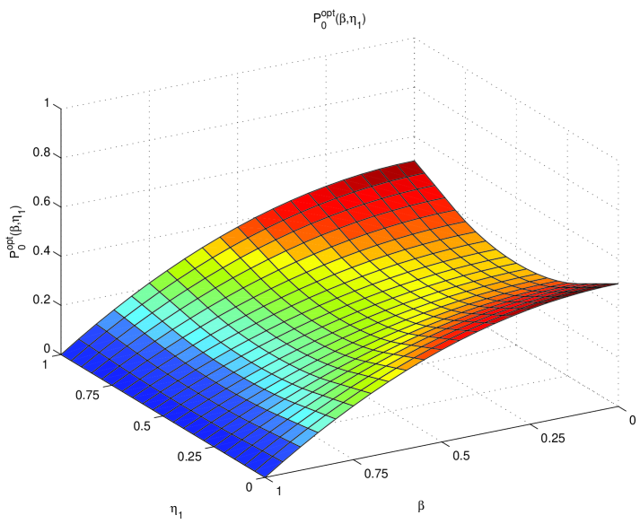
(a) $P_{0}^{opt}(\beta,\eta_{1})$

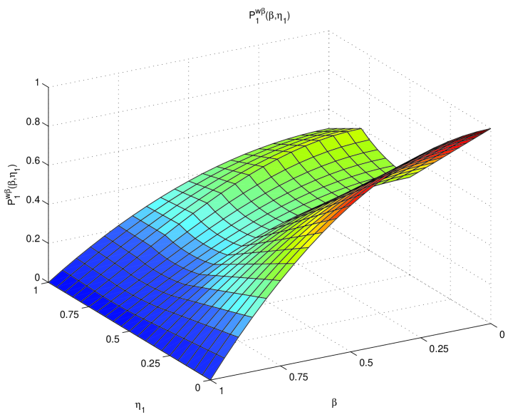
(b) $P_{1}^{w\beta}(\beta,\eta_{1})$

(c) $P_{1+}^{opt}(\beta,\eta_{1})$

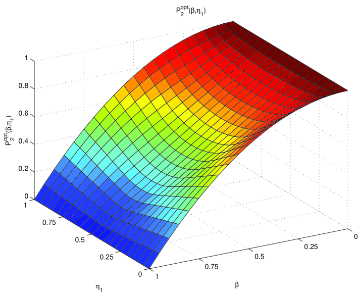
(d) $P_{2}^{opt}(\beta,\eta_{1})$

Figure 1: Optimum success probabilities: $P_{0}^{opt}(\beta,\eta_{1})$, $P_{1}^{w\beta}(\beta,\eta_{1})$, $P_{1+}^{opt}(\beta,\eta_{1})$ and $P_{2}^{opt}(\beta,\eta_{1})$

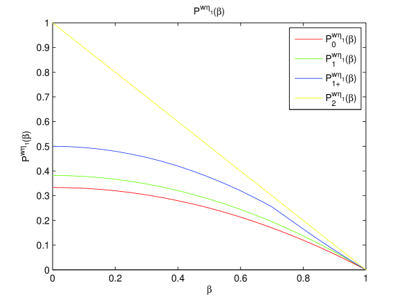
Figure 2: $P_{0}^{w\eta_{1}}(\beta)$, $P_{1}^{w\beta\eta_{1}}(\beta)$, $P_{1+}^{w\eta_{1}}(\beta)$ and $P_{2}^{w\eta_{1}}(\beta)$ and their images.

To make even clearer comparison, we further plot two-parameter functions $P_{0}^{w\eta_{1}}(\beta,\eta_{1})$, $P_{1}^{w\beta\eta_{1}}(\beta,\eta_{1})$, $P_{1+}^{w\eta_{1}}(\beta,\eta_{1})$ and $P_{2}^{w\eta_{1}}(\beta,\eta_{1})$ in Fig. 3.

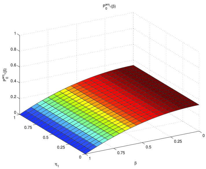
(a) $P_{0}^{w\eta_{1}}(\beta,\eta_{1})$

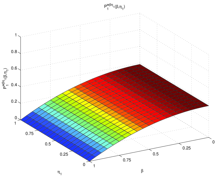
(b) $P_{1}^{w\beta\eta_{1}}(\beta,\eta_{1})$

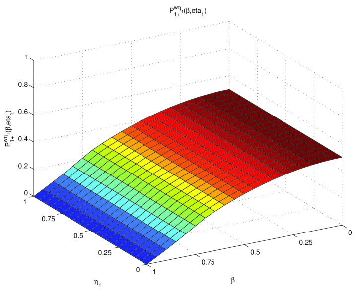
(c) $P_{1+}^{w\eta_{1}}(\beta,\eta_{1})$

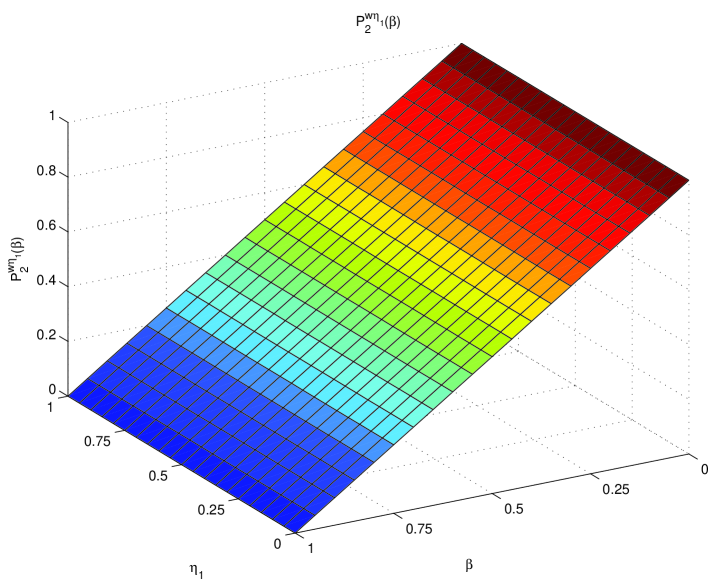
(d) $P_{2}^{w\eta_{1}}(\beta,\eta_{1})$

Figure 3: Optimum success probabilities: $P_{0}^{w\eta_{1}}(\beta,\eta_{1})$, $P_{1}^{w\beta\eta_{1}}(\beta,\eta_{1})$, $P_{1+}^{w\eta_{1}}(\beta,\eta_{1})$ and $P_{2}^{w\eta_{1}}(\beta,\eta_{1})$

3.2.1 The effect of a priori probabilities on optimum performances

By comparing the optimal performance $P_{0}^{opt}(\beta,\eta_{1})$ (see Fig. 1(a)) in Case A1 with $P_{0}^{w\eta_{1}}(\beta,\eta_{1})$ (Fig. 3(a)) in Case B1, it is demonstrated that the former is better than the latter as shown in Fig. 4(a). This implies that a priori probability can be utilized to improve the optimum performance even when the two discriminated states are classically unknown, yet we have a copy of them.

By comparing the optimal performance $P_{1}^{w\beta}(\beta,\eta_{1})$(Fig. 1(b)) in Case A2 with $P_{1}^{w\beta\eta_{1}}(\beta,\eta_{1})$ (see Fig. 3(b)) in Case B2, the former is found to be better than the latter as shown in Fig. 4(b). It is also easy to find in Fig. 4(c) that the optimal performance $P_{1+}^{opt}(\beta,\eta_{1})$ (see Fig. 1(c))in Case A3 is better than $P_{1+}^{w\eta_{1}}(\beta,\eta_{1})$ (see Fig. 3(c)) in Case B3. This implies that the a priori probability can be utilized to improve the optimum performance when one only has partial a priori classical knowledge of the discriminated states.

In the comparing Figure 4(d) between the optimal performance $P_{2}^{opt}(\beta,\eta_{1})$ (see Fig. 1(d)) in Case A4 and $P_{2}^{w\eta_{1}}(\beta,\eta_{1})$ (see Fig. 3(d)) in Case B4, the same conclusion can be addressed, i.e., the former is clearly better than the latter. This implies that the knowledge of a priori probability can be utilized to improve the optimum performance when we have a priori complete classical knowledge of the discriminated states.

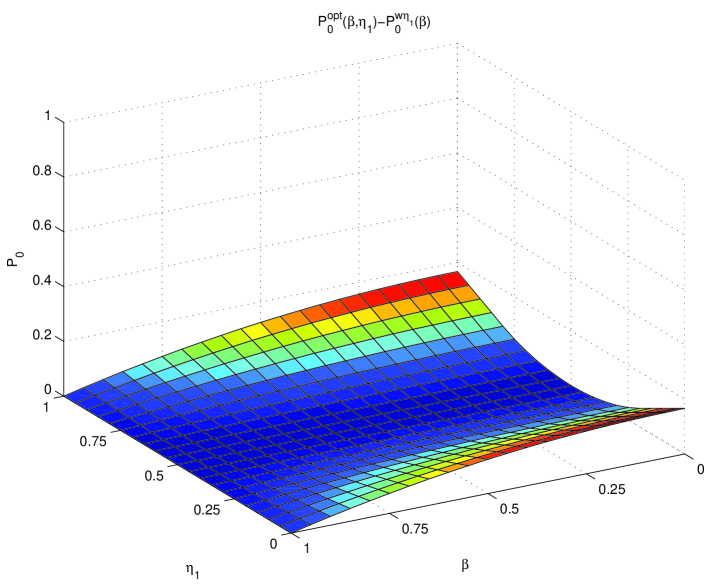
(a) $P_{0}^{w\eta_{1}\rightarrow\eta_{1}}(\beta,\eta_{1})$

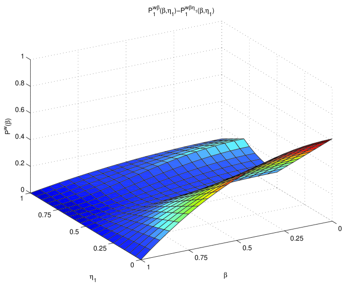
(b) $P_{1}^{w\eta_{1}\rightarrow\eta_{1}}(\beta,\eta_{1})$

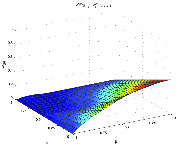
(c) $P_{1+}^{w\eta_{1}\rightarrow\eta_{1}}(\beta,\eta_{1})$

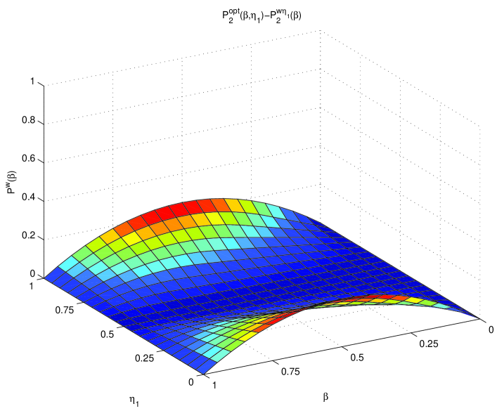
(d) $P_{2}^{w\eta_{1}\rightarrow\eta_{1}}(\beta,\eta_{1})$

Figure 4: Improving optimum success probabilities: $P_{0}^{w\eta_{1}\rightarrow\eta_{1}}(\beta,\eta_{1})$, $P_{1}^{w\eta_{1}\rightarrow\eta_{1}}(\beta,\eta_{1})$, $P_{1+}^{w\eta_{1}\rightarrow\eta_{1}}(\beta,\eta_{1})$ and $P_{2}^{w\eta_{1}\rightarrow\eta_{1}}(\beta,\eta_{1})$

3.2.2 The effect of classical knowledge on optimum performances

As shown in Fig. 5(a), the optimal performance $P_{0}^{opt}(\beta,\eta_{1})$ (see Fig. 1(a)) in Case A1 is better than $P_{1}^{w\beta}(\beta,\eta_{1})$ (Fig. 1(b)) in Case A2, and naturally the optimal performance $P_{1+}^{opt}(\beta,\eta_{1})$ (Fig. 1(c)) in Case A3 is better than $P_{1}^{w\beta}(\beta,\eta_{1})$ (Fig. 1(b)) in Case A2, as shown in Fig. 5(b), the optimal performance $P_{1+}^{opt}(\beta,\eta_{1})$ (Fig. 1(c)) in Case A3 is better than $P_{2}^{opt}(\beta,\eta_{1})$ (see Fig. 1(d)) in Case A4, as shown in Fig. 5(c). This implies that the classical knowledge of discriminated states can be utilized to improve the optimum performance when we have a priori probability of preparing the discriminated states.

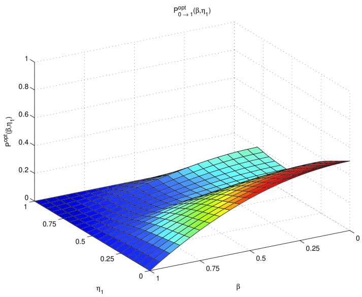
(a) $P_{0\rightarrow 1}^{opt}(\beta,\eta_{1})$

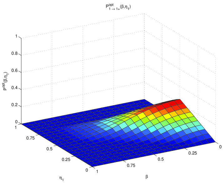
(b) $P_{1\rightarrow 1+}^{opt}(\beta,\eta_{1})$

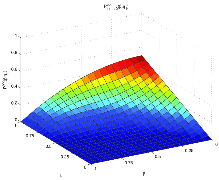
(c) $P_{1+\rightarrow 2}^{opt}(\beta,\eta_{1})$

Figure 5: Performance-improving functions $P_{0\rightarrow 1}^{opt}(\beta,\eta_{1})$, $P_{1\rightarrow 1+}^{opt}(\beta,\eta_{1})$ and $P_{1+\rightarrow 2}^{opt}(\beta,\eta_{1})$

It is observed in Fig. 6 that the optimum performance increases with the amount of classical knowledge of discriminated states provided even when a priori probabilities of preparing the discriminated states are unknown.

By comparing the optimal performance $P_{0}^{w\eta_{1}}(\beta,\eta_{1})$ (see Fig. 3(a))in Case B1 with $P_{1}^{w\beta\eta_{1}}(\beta,\eta_{1})$ (Fig. 3(b)) in Case B2, the latter is better than the former as shown in Fig. 6(a). It is not difficult to predict the same situation in Fig. 6(b) and Fig.6(c) when comparing the optimal performance $P_{1+}^{w\eta_{1}}(\beta,\eta_{1})$ (Fig. 3(c)) in Case B3 with $P_{1}^{w\beta\eta_{1}}(\beta,\eta_{1})$ (Fig. 3(b)) in Case B2, and when comparing the optimal performance $P_{1+}^{w\eta_{1}}(\beta,\eta_{1})$ (see Fig. 3(c)) in Case B3 with $P_{2}^{w\eta_{1}}(\beta,\eta_{1})$ (see Fig. 3(d)) in Case B4.

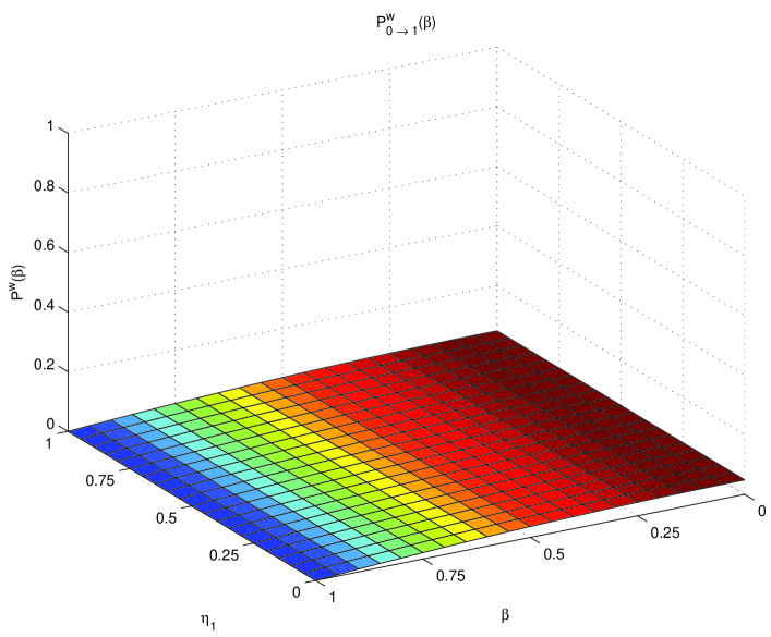
(a) $P_{0\rightarrow 1}^{w\eta_{1}}(\beta,\eta_{1})$

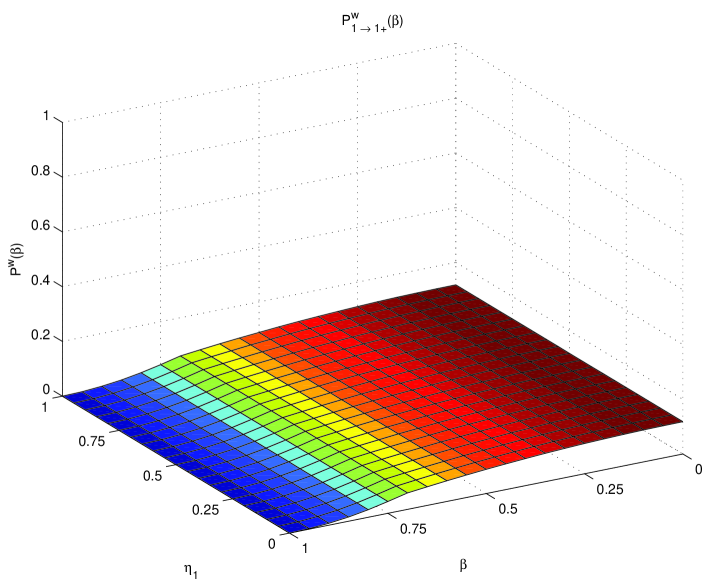
(b) $P_{1\rightarrow 1+}^{w\eta_{1}}(\beta,\eta_{1})$

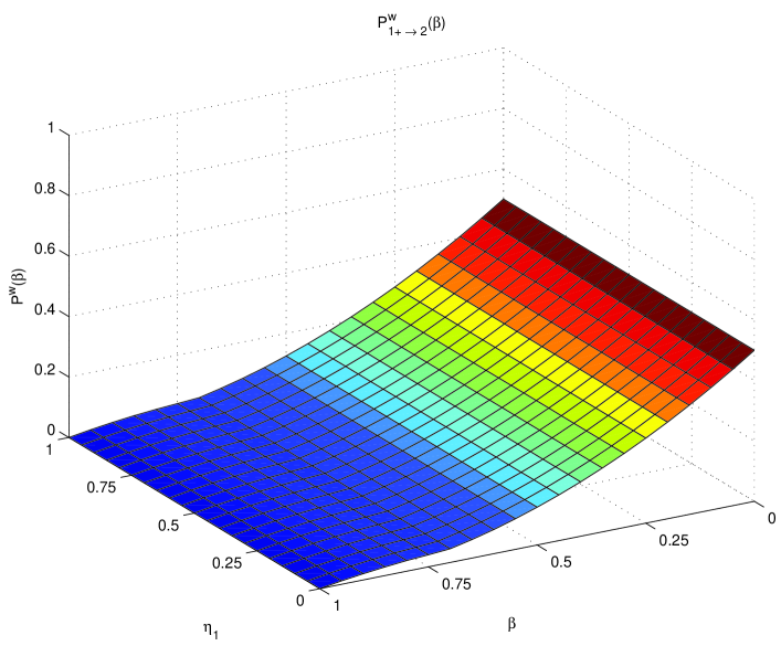
(c) $P_{1+\rightarrow 2}^{w\eta_{1}}(\beta,\eta_{1})$

Figure 6: Two-parameter performance-improving functions $P_{0\rightarrow 1}^{w\eta_{1}}(\beta,\eta_{1})$, $P_{1\rightarrow 1+}^{w\eta_{1}}(\beta,\eta_{1})$ and $P_{1+\rightarrow 2}^{w\eta_{1}}(\beta,\eta_{1})$

4 Optimal unambiguous discrimination problems for two qutrit states

To further clarify the effect of a priori information of the discriminated states on optimum unambiguous discriminators and optimum success probabilities, we will study optimum unambiguous discrimination problems for two qutrit states in this section. At first, we will present the results on optimal unambiguous discrimination problems with the knowledge of a priori preparing probabilities in the first three subsections. According to what kind of classical knowledge can be utilized, the 4 cases are discussed as follows

Case A1, without classical knowledge of either state but with a single copy of unknown states;

Case A2, with only classical knowledge of one of the two states and a single copy of the other unknown state;

Case A3, with only classical knowledge of one of the two states and the absolute value of the inner product of both states, and also with a single copy of the other unknown state;

Case A4, with classical knowledge of both states.

The A1 and A4 cases will be investigated in subsection A and C, respectively, and the A2 and A3 cases will be studied in subsection B.

Furthermore, optimal unambiguous discrimination problems without a priori preparing probability will be investigated in the subsection D, E, F. Corresponding to what will be explored in the subsection A, B and C, we have also four cases taken into consideration as follow.

Case B1, without classical knowledge of either state but with a single copy of unknown states;

Case B2, with classical knowledge of one of the two states and a single copy of the other unknown state;

Case B3, with classical knowledge of one of the two states and the absolute value of the inner product of both states, and also with a single copy of the other unknown state;

Case B4, with classical knowledge of both states.

The B1 and B4 cases will be investigated in subsection D and F, respectively, and the B2 and B3 cases will be studied in subsection E.

4.1 Optimal unambiguous discrimination problems for Case A1

In this subsection, we first consider the optimal unambiguous discrimination problems for two qutrit states. The preparing probabilities is given, but none classical knowledge of discriminated states is available.

The procedure of analysis is in line with Section II. A, but there is some difference between them in how to construct the measurement operators.

Since we have no classical knowledge about two qutrits $|\psi_{1}\rangle$ and $|\psi_{2}\rangle$, the right way of constructing POVM operators is to take advantage of the symmetrical properties of the states. Denoting $|0\rangle$, $|1\rangle$ and $|2\rangle$ as three vectors of a basis, we define the antisymmetric states as follows

$$|\psi_{BC1}^{-}\rangle=\frac{1}{\sqrt{2}}(|0\rangle_{B}|1\rangle_{C}-|1\rangle_{B}|0\rangle_{C})$$ (79)

and

$$|\psi_{BC2}^{-}\rangle=\frac{1}{\sqrt{2}}(|0\rangle_{B}|2\rangle_{C}-|2\rangle_{B}|0\rangle_{C})$$ (80)

and

$$|\psi_{BC3}^{-}\rangle=\frac{1}{\sqrt{2}}(|1\rangle_{B}|2\rangle_{C}-|2\rangle_{B}|1\rangle_{C})$$ (81)

and

$$|\psi_{AB1}^{-}\rangle=\frac{1}{\sqrt{2}}(|0\rangle_{A}|1\rangle_{B}-|1\rangle_{A}|0\rangle_{B})$$ (82)

and

$$|\psi_{AB2}^{-}\rangle=\frac{1}{\sqrt{2}}(|0\rangle_{A}|2\rangle_{B}-|2\rangle_{A}|0\rangle_{B})$$ (83)

and

$$|\psi_{AB2}^{-}\rangle=\frac{1}{\sqrt{2}}(|1\rangle_{A}|2\rangle_{B}-|2\rangle_{A}|1\rangle_{B})$$ (84)

and introduce the projectors to the antisymmetric subspaces of the corresponding qutrit as

$${P}_{BCi}^{as}=|\psi_{BCi}^{-}\rangle\langle\psi_{BCi}^{-}|$$ (85)

and

$${P}_{ABi}^{as}=|\psi_{ABi}^{-}\rangle\langle\psi_{ABi}^{-}|$$ (86)

with $i=1,2,3$. We now can take for ${\Pi}_{1}$ and ${\Pi}_{2}$ operators

$${\Pi}_{1}=\sum^{3}_{i=1}\lambda_{1i}I_{A}\otimes{P}_{BCi}^{as}$$ (87)

and

$${\Pi}_{2}=\sum^{3}_{i=1}\lambda_{2i}{P}_{ABi}^{as}\otimes{I_{C}}$$ (88)

To assure that ${\Pi}_{1}$, ${\Pi}_{2}$ and ${\Pi}_{0}=I-{\Pi}_{1}-{\Pi}_{2}$ be semi-positive operators, the following constraints should be satisfied:

$$2-\lambda_{1i}-\lambda_{2i}\geq 0;\ 1-\lambda_{1i}-\lambda_{2i}+\frac{3}{4}\lambda_{1i}\lambda_{2i}\geq 0$$ (89)

with $i=1,2,3$.

Since we have knowledge of $\eta_{1}$, our task is reduced to designing $\lambda_{1i}(\eta_{1})$ and $\lambda_{2i}(\eta_{1})$ such that the following average success probability

$$P=\eta_{1}p_{1}+(1-\eta_{1})p_{2}$$ (90)

is maximal with the constrains given by Eq. (89).

In this case, the corresponding optimal action parameters are given by

$$\lambda_{1i}^{0,opt}(\eta_{1})=\ \bigg{\{}\begin{array}[]{cc}0&\eta_{1}\leq{\frac{1}{5}}\\ \frac{2}{3}[2-\sqrt{\frac{1-\eta_{1}}{\eta_{1}}}]&\frac{1}{5}\leq{\eta_{1}}\leq{\frac{4}{5}}\\ 1&\eta_{1}\geq{\frac{4}{5}}\end{array}$$ (91)

and

$$\lambda_{2i}^{0,opt}(\eta_{1})=\ \bigg{\{}\begin{array}[]{cc}1&\eta_{1}\leq{\frac{1}{5}}\\ \frac{2}{3}[2-\sqrt{\frac{\eta_{1}}{1-\eta_{1}}}]&\frac{1}{5}\leq{\eta_{1}}\leq{\frac{4}{5}}\\ 0&\eta_{1}\geq{\frac{4}{5}}\end{array}$$ (92)

with $i=1,2,3$ and the optimum success probability $P_{0}^{opt}$ can be computed as follows

$$\sum^{3}_{i=1}\lambda_{1i}^{0,opt}\langle\Psi_{1}^{in}|I_{A}\otimes{P}_{BCi}^{as}|\Psi_{1}^{in}\rangle+\sum^{3}_{i=1}\lambda_{2i}^{0,opt}\langle\Psi_{2}^{in}|{P}_{ABi}^{as}\otimes{I_{C}}|\Psi_{2}^{in}\rangle$$ (93)

where the subscript $0$ of $P_{0}^{opt}$ means that we have no a priori classical knowledge of $|\psi_{1}\rangle$ and $|\psi_{2}\rangle$.

Remark: From the aforementioned analysis, we reveal that the measurement operators for discriminating two qutrit states are more complicated than those for the qubit case. In general, it is also impossible to express the optimum success probability $P_{0}^{opt}$ as the function of $\beta$ and $\eta_{1}$.

4.2 Optimal unambiguous discrimination problems for A2 and A3

In this subsection, we studied the optimal unambiguous discrimination problem of for the cases A2 and A3.

The analysis is similar with Section II. B, but the key challenge is how to construct the measurement operators for qutrit states.

Since we know nothing about $|\psi_{2}\rangle$ but have the classical knowledge of $|\psi_{1}\rangle$, the right way of constructing POVM operators is to take advantage of the symmetrical properties of the state as well as the classical knowledge of $|\psi_{1}\rangle$. Denote $|\psi_{1}\rangle=|0\rangle$, and Let $|0\rangle$, $|1\rangle$ and $|2\rangle$ constitute a basic basis. We define the antisymmetric state

$$|\psi_{AB1}^{-}\rangle=\frac{1}{\sqrt{2}}(|0\rangle_{A}|1\rangle_{B}-|1\rangle_{A}|0\rangle_{B})$$ (94)

and

$$|\psi_{AB2}^{-}\rangle=\frac{1}{\sqrt{2}}(|0\rangle_{A}|2\rangle_{B}-|2\rangle_{A}|0\rangle_{B})$$ (95)

and introduce the projectors to the antisymmetric subspaces of the corresponding qubit as

$${P}_{ABi}^{as}=|\psi_{ABi}^{-}\rangle\langle\psi_{ABi}^{-}|$$ (96)

with $i=1,2$.

By making full use of the knowledge of $|\psi_{1}\rangle$, we construct the measurement operators ${\Pi}_{1}$ and ${\Pi}_{2}$ to satisfy the no-error condition given by Eq.(5) as follows:

$${\Pi}_{1}=\sum^{2}_{i=1}\lambda_{1i}{P}_{ABi}^{as}$$ (97)

and

$${\Pi}_{2}=\sum^{2}_{i=1}\lambda_{2i}{|0\rangle_{A}|i\rangle_{B}{{}_{B}\langle}i|_{A}\langle{0}|}+\sum^{2}_{j,k=1}\lambda_{3jk}{|j\rangle_{A}|k\rangle_{B}{{}_{B}\langle}k|_{A}\langle{j}|}$$ (98)

where $\lambda_{1i}$, $\lambda_{2i}$ and $\lambda_{3jk}$ are undetermined nonnegative real numbers. In terms of Eqs. (97) and (98), we can obtain the values of $p_{1}$ and $p_{2}$ by means of Eqs. (3) and (4).

By assuming that the preparation probabilities of $|\psi_{1}\rangle$ and $|\psi_{2}\rangle$ are $\eta_{1}$ and $\eta_{2}$ (where $\eta_{2}=1-\eta_{1}$), respectively, we can still define the average probability $P$ of successfully discriminating two states as

$$P=\eta_{1}p_{1}+(1-\eta_{1})p_{2}$$ (99)

and our task is to maximize the performance Eq. (99) subject to the constraint that ${\Pi}_{0}=I-{\Pi}_{1}-{\Pi}_{2}$ is a positive operator. After some calculations, we have

$$p_{1}=\sum^{2}_{i=1}\lambda_{1i}|\langle\psi_{2}|i\rangle|^{2}$$ (100)

and

$$p_{2}=\sum^{2}_{i=1}\lambda_{2i}\beta^{2}|\langle\psi_{2}|i\rangle|^{2}+\sum^{2}_{j,k=1}\lambda_{3jk}|\langle\psi_{2}|j\rangle|^{2}|\langle\psi_{2}|k\rangle|^{2}$$ (101)

To assure that operators ${\Pi}_{0}$, ${\Pi}_{1}$ and ${\Pi}_{2}$ are positive operators, we have the following inequality constraints:

$$1-{\lambda_{1i}}-{\lambda_{2i}}+\frac{1}{2}{\lambda_{1i}}{\lambda_{2i}}\geq 0$$ (102)

and

$$0\leq{\lambda_{1i},\lambda_{2i},\lambda_{3jk}}\leq 1(i,j,k=1,2)$$ (103)

Based on the aforementioned observations, we can give some further analysis. Subsequently, we will discuss our strategies for the A2 and A3 cases.

(i) For the A2 case, we have the knowledge of preparing probability $\eta_{1}$, but no knowledge of $\beta$.

Our strategy is to design $\lambda^{1,w\beta}_{1i}(\eta)$, $\lambda^{1,w\beta}_{2i}(\eta)$ and $\lambda^{1,w\beta}_{3jk}(\eta)$ to maximize the minimal performance

$$J=\max\min_{\{\beta\}}[\eta_{1}p_{1}+(1-\eta_{1})p_{2}]$$ (104)

subject to the constraints described by Eqs. (102) and (103).

No matter what $\eta_{1}$ is, one should always choose $\lambda^{1,w\beta}_{3jk}(\eta_{1})=1$. Fortunately, this problem can be reduced to maximizing the minimal performance

$$J_{i}=\max\min_{\{\beta\}}[\frac{1}{2}\eta_{1}\lambda_{1i}+(1-\eta_{1})\lambda_{2i}\beta^{2}]$$ (105)

subject to the constraints described by Eqs. (102) and

$$0\leq{\lambda_{1i},\lambda_{2i}}\leq 1(i,j,k=1,2)$$ (106)

After some calculation, we have

$$\lambda_{1i}^{1,w\beta}(\eta_{1})=\ \bigg{\{}\begin{array}[]{cc}0&\eta_{1}\leq{\frac{1}{2}}\\ 2(1-\sqrt{\frac{1-\eta_{1}}{\eta_{1}}})&\frac{1}{2}\leq{\eta_{1}}\leq{\frac{4}{5}}\\ 1&\eta_{1}\geq{\frac{4}{5}}\end{array}$$ (107)

and

$$\lambda_{2i}^{1,w\beta}(\eta_{1})=\ \bigg{\{}\begin{array}[]{cc}1&\eta_{1}\leq{\frac{1}{2}}\\ 2-\sqrt{\frac{\eta_{1}}{1-\eta_{1}}}&\frac{1}{2}\leq{\eta_{1}}\leq{\frac{4}{5}}\\ 0&\eta_{1}\geq{\frac{4}{5}}\end{array}$$ (108)

and

$$\lambda^{1,w\beta}_{3jk}(\eta_{1})=1$$ (109)

By substituting $\lambda^{1,w\beta}_{1i}(\eta_{1})$, $\lambda^{{1,w\beta}}_{2i}(\eta_{1})$ and $\lambda^{1,{w\beta}}_{3jk}(\eta_{1})$ into (99), we obtain the actual optimum success probability $P_{1}^{w\beta}$in this strategy: where the subscript $1$ of $P_{1}^{w\beta}$ means that we just have a priori classical knowledge of $|\psi_{1}\rangle$, one of two discriminated states, and the superscript $w\beta$ of $P_{1}^{w\beta}$ implies that the optimum success probability is obtained when making the decision based on the worst case for $\beta$.

Remark: In this case, we can still choose the parameters of the measurement operators based on the knowledge of a priori probability of the discriminated states. It should be pointed out that the inner product of two discriminated qutrit states still plays the the same role in optimum unambiguous state discrimination problems as that of two qubit states.

(ii) With a priori classical knowledge of both $|\langle\psi_{1}|\psi_{2}\rangle|=\beta$ and $\eta_{1}$ in hand, our task in the third case is to get the optimum values $\lambda^{1+,opt}_{1i}(\beta,\eta_{1})$, $\lambda^{1+,opt}_{2i}(\beta,\eta_{1})$ and $\lambda^{1+,opt}_{3jk}(\beta,\eta_{1})$ to optimize the average success probability

$$P=\eta_{1}p_{1}+(1-\eta_{1})p_{2}$$ (110)

subject to the constraints described by Eqs. (102) and (103).

No matter what $\eta_{1}$ is, one should always choose $\lambda^{1+,opt}_{3jk}(\eta_{1},\beta)=1$. Fortunately, this problem can be reduced to choosing $\lambda^{1+,opt}_{1i}(\beta,\eta_{1})$ and , $\lambda^{1+,opt}_{2i}(\beta,\eta_{1})$ to maximize performance

$$J_{i}=\frac{1}{2}\eta_{1}\lambda_{1i}+(1-\eta_{1})\lambda_{2i}\beta^{2}$$ (111)

subject to the constraints described by Eqs. (102) and (106).

After some calculations, we have

$$\lambda^{1+,opt}_{1i}(\beta,\eta_{1})=\ \bigg{\{}\begin{array}[]{cc}0&\eta_{1}\leq\frac{{\beta}^{2}}{1+{\beta}^{2}}\\ 2(1-\beta\sqrt{\frac{1-\eta_{1}}{\eta_{1}}})&\frac{{\beta}^{2}}{1+{\beta}^{2}}\leq{\eta_{1}}\leq{\frac{4{\beta}^{2}}{1+4{\beta}^{2}}}\\ 1&\eta_{1}\geq{{\frac{4{\beta}^{2}}{1+4{\beta}^{2}}}}\end{array}$$ (112)

and

$$\lambda^{1+,opt}_{2i}(\beta,\eta_{1})=\ \bigg{\{}\begin{array}[]{cc}1&\eta_{1}\leq\frac{{\beta}^{2}}{1+{\beta}^{2}}\\ 2-\frac{1}{\beta}\sqrt{\frac{\eta_{1}}{1-\eta_{1}}}&\frac{{\beta}^{2}}{1+{\beta}^{2}}\leq{\eta_{1}}\leq{\frac{4{\beta}^{2}}{1+4{\beta}^{2}}}\\ 0&\eta_{1}\geq{{\frac{4{\beta}^{2}}{1+4{\beta}^{2}}}}\end{array}$$ (113)

and

$$\lambda^{1+,opt}_{3jk}(\beta,\eta_{1})\equiv 1$$ (114)

Taking Eq. (110) into consideration, we obtain the corresponding optimum success probabilities $P_{1+}^{opt}(\beta,\eta_{1})$: where the subscript $1+$ of $P_{1+}^{opt}$ means that we have a priori classical knowledge of one of the two discriminated states and the absolute value of the inner product of the two states.

Remark: It is interesting to underline that it is impossible to express the optimum success probability $P_{1+}^{opt}$ as the function of the inner product of two qutrit states $\beta$ and a priori preparing probability $\eta_{1}$, but one can make the optimum decision just based on the knowledge of $\beta$ and $\eta_{1}$.

4.3 Optimal unambiguous discrimination problems for Case A4

If we have complete a priori classical knowledge of both $|\psi_{1}\rangle$ and $|\psi_{2}\rangle$, the measurement is performed on the detected qutrit. One can select the detection operators as follows:

(1) Select $|0\rangle=|\psi_{1}\rangle$, and choose another two state $|1^{\prime}\rangle$ and $|2^{\prime}\rangle$ so that the three states $|0\rangle$, $|1^{\prime}\rangle$ and $|2^{\prime}\rangle$ constitute a set of basis base.

(2) Express $|\psi_{2}\rangle$ in terms of $|0\rangle$, $|1^{\prime}\rangle$ and $|2^{\prime}\rangle$ as follows:

$$|\psi_{2}\rangle=\cos\frac{\theta_{1}}{2}|0\rangle+e^{i\phi^{\prime}_{1}}\sin\frac{\theta_{1}}{2}\cos\frac{\theta_{2}}{2}|1^{\prime}\rangle+e^{i\phi^{\prime}_{2}}\sin\frac{\theta_{1}}{2}\sin\frac{\theta_{2}}{2}|2^{\prime}\rangle$$ (115)

By setting

$$|1\rangle=e^{i\phi^{\prime}_{1}}\cos\frac{\theta_{2}}{2}|1^{\prime}\rangle+e^{i\phi^{\prime}_{2}}\sin\frac{\theta_{2}}{2}|2^{\prime}\rangle$$ (116)

$$|2\rangle=e^{i\phi^{\prime}_{2}}\sin\frac{\theta_{2}}{2}|1^{\prime}\rangle-e^{i\phi^{\prime}_{1}}\sin\frac{\theta_{2}}{2}|2^{\prime}\rangle$$ (117)

we have

$$|\psi_{2}\rangle=\cos\frac{\theta_{1}}{2}|0\rangle+\sin\frac{\theta_{1}}{2}|1\rangle$$ (118)

and the three states $|0\rangle$, $|1\rangle$ and $|2\rangle$ constitute another set of basis base.

(3)

$${\Pi}_{1}=\lambda_{1}{|e_{1}\rangle\langle{e_{1}}|}$$ (119)

with $|e_{1}\rangle=\sin\frac{\theta_{1}}{2}|0\rangle-\cos\frac{\theta_{1}}{2}|1\rangle$ and

$${\Pi}_{2}=\lambda_{2}{|1\rangle\langle 1|}$$ (120)

Denote $\cos\frac{\theta_{1}}{2}=\beta$, we have $|\langle\psi_{1}|\psi_{2}\rangle|=\beta$. Our task is still to choose $\lambda_{1}$ and $\lambda_{2}$ based on a priori information such that the average success probability given by Eq. (52) is maximized.

To assure that ${\Pi}_{0}=I-{\Pi}_{1}-{\Pi}_{2}$, ${\Pi}_{1}$ and ${\Pi}_{2}$ are positive operators, we still have the inequality constraints given by Eqs.(54-55).

Since we have knowledge of preparing probability $\eta_{1}$ and $\beta$, we will make the decision given by Eqs.(56-57)

Furthermore, we can obtain the optimum success probability Eq. (58) with Eqs.(59-61) where the subscript $2$ of $P_{2}^{opt}$ still means that we have the classical knowledge of both discriminated states.

Remark: It is interesting to point out that the optimal unambiguous discrimination problem for two qutrit states can be reduce to the same one for two qubit states when the classical knowledge of both discriminated states is available.

4.4 Optimal unambiguous discrimination problems for Case B1

Since we have the same classical knowledge of discriminated states in this case as in Section IV. A, we can follow the analysis in Section IV. A and choose ${\Pi}_{1}$ and ${\Pi}_{2}$ as Eqs. (87) and (88).

To assure that ${\Pi}_{1}$, ${\Pi}_{2}$ and ${\Pi}_{0}=I-{\Pi}_{1}-{\Pi}_{2}$ be semi-positive operators, the constraints on $\lambda_{1}$ and $\lambda_{2}$ described by Eq.(89) should be satisfied.

However, since we have no knowledge of preparing probability, we have to design $\lambda_{1}$ and $\lambda_{2}$ without a priori information of $\eta_{1}$. Our strategy is to maximize the minimal performance

$$J=P_{0}^{w\eta_{1}}=\max\min_{\{\eta_{1}\}}\{\eta_{1}p_{1}+(1-\eta_{1})p_{2}\}$$ (121)

with the constraints in Eq. (89).

After careful calculations, we obtain that

$$\lambda^{{0,w\eta_{1}}}_{1i}=\lambda^{0,w\eta_{1}}_{2i}=\frac{2}{3}$$ (122)

Substituting Eq. (122) into Eq. (121) yields $P_{0}^{w\eta_{1}}$.

4.5 Optimal unambiguous discrimination problems for Cases B2 and B3

In this subsection, we will discuss the optimal unambiguous discrimination problems for the B2 and B3 cases where partial classical knowledge but none knowledge of preparing probabilities of discriminated states are available.

Since we have the same partial classical knowledge of discriminated states in this section as in Section IV.B, we can follow the analysis in Section IV.B and choose ${\Pi}_{1}$ and ${\Pi}_{2}$ as Eqs.(97) and (98).

To assure that ${\Pi}_{1}$, ${\Pi}_{2}$ and ${\Pi}_{0}=I-{\Pi}_{1}-{\Pi}_{2}$ be semi-positive operators, the constraints on $\lambda_{1i}$, $\lambda_{2i}$ and $\lambda_{3jk}$ described by (102) and (103) should be satisfied.

Our task is to design$\lambda_{1i}$, $\lambda_{2i}$ and $\lambda_{3jk}$ such that the average success probability

$$P=\eta_{1}p_{1}+(1-\eta_{1})p_{2}$$ (123)

is maximized.

Subsequently, we will discuss our strategies for the B2 and B3 cases, respectively.

(i) If we have neither the knowledge of preparing probabilities nor the knowledge of $\beta$, our task is reduced to designing $\lambda_{1i}^{1,w\beta\eta_{1}}$, $\lambda_{2i}^{1,w\beta\eta_{1}}$ and $\lambda_{3jk}^{1,w\beta\eta_{1}}$ to maximize the minimal performance Eq.(123) subject to the constraints in Eqs. (102) and (103).

No matter what $\eta_{1}$ is, one should always choose $\lambda^{1,w\beta\eta_{1}}_{3jk}(\eta_{1})=1$. Fortunately, this problem can be further reduced to maximizing the minimal performance

$$J_{i}=\max\min_{\{\beta,\eta_{1}\}}[\frac{1}{2}\eta_{1}\lambda_{1i}+(1-\eta_{1})\lambda_{2i}\beta^{2}]$$ (124)

subject to the constraints described by Eqs. (102) and (106).

Following some calculations in the subsection IV. B, we have the optimal actions as follows

$$\lambda_{1i}^{1,w\beta\eta_{1}}=3-\sqrt{5}$$ (125)

and

$$\lambda_{2i}^{1,w\beta\eta_{1}}=\frac{1}{2}(3-\sqrt{5})$$ (126)

and

$$\lambda_{3jk}^{1,w\beta\eta_{1}}=1$$ (127)

By substituting them into Eq. (99), we get the actual optimum success probability $P_{1}^{w\beta\eta_{1}}$ where the subscript $1$ of $P_{1}^{w\beta\eta_{1}}$ means that we just have a priori classical knowledge of $|\psi_{1}\rangle$, one of two discriminated states, and the superscript $w\beta\eta_{1}$ implies that the optimum success probability is obtain based on the decision for the worst case for both $\beta$ and $\eta_{1}$.

Remark: Although the actual optimum success probability $P_{1}^{w\beta\eta_{1}}$ depends on the both $\beta$ and $\eta_{1}$, the optimum decision given by Eqs. (125-127) is independent of $\beta$ and $\eta_{1}$.

(ii) For the B3 case, we have the knowledge of $\beta$, but no knowledge of preparing probability $\eta_{1}$.

Our task is to design $\lambda^{1+,w\eta_{1}}_{1}(\beta)$, $\lambda^{1+,w\eta_{1}}_{2}(\beta)$ and $\lambda^{1+,w\eta_{1}}_{3}(\beta)$ to maximize the minimal performance

$$J=\max\min_{\{\eta_{1}\}}[p_{1}\eta_{1}+p_{2}(1-\eta_{1})]$$ (128)

subject to the constraints given by Eqs. (32) and (33).

No matter what $\eta_{1}$ is, one should always choose $\lambda^{1,w\eta_{1}}_{3jk}(\beta)=1$. Fortunately, this problem can be further reduced to maximizing the minimal performance

$$J_{i}=\max\min_{\{\eta_{1}\}}[\frac{1}{2}\eta_{1}\lambda_{1i}+(1-\eta_{1})\lambda_{2i}\beta^{2}]$$ (129)

subject to the constraints described by Eqs. (102) and (106).

Following some similar calculations in subsection II. E, we have

$$\lambda_{1i}^{1+,w\eta_{1}}(\beta)=\ \bigg{\{}\begin{array}[]{cc}1&\beta\leq\frac{\sqrt{2}}{2}\\ \beta^{2}+2-\sqrt{\beta^{4}+4\beta^{2}}&\beta\geq\frac{\sqrt{2}}{2}\end{array}$$ (130)

and

$$\lambda_{2i}^{1+,w\eta_{1}}(\beta)=\ \bigg{\{}\begin{array}[]{cc}0&\beta\leq\frac{\sqrt{2}}{2}\\ \frac{3}{2}-\sqrt{\frac{1}{4}+\frac{1}{\beta^{2}}}&\beta\geq\frac{\sqrt{2}}{2}\end{array}$$ (131)

and

$$\lambda_{3jk}^{1+,w\eta_{1}}(\beta)\equiv 1$$ (132)

By substituting $\lambda^{1+,w\eta_{1}}_{1i}$, $\lambda^{{1+,w\eta_{1}}}_{2i}$ and $\lambda^{1+,{w\eta_{1}}}_{3jk}$ into (99), we obtain the actual success probability $P_{1+}^{A}(\beta,\eta_{1})$ and optimum success probabilities in the worst case $P_{1+}^{w\eta_{1}}$.

Remark: In this case, the optimum decision given by Eqs. (130-132) is only the function of $\beta$.

4.6 Optimal unambiguous discrimination problems for case B4

This subsection discuss the optimal unambiguous discrimination problem where complete classical knowledge of discriminated states but none a priori probabilities of preparing the discriminated states are available.

Here we have the same classical knowledge of discriminated states in this case as in Section IV. C, thus we can follow the analysis in Section IV. C and choose ${\Pi}_{1}$ and ${\Pi}_{2}$ as Eqs. (119) and (120).

In order to assure that ${\Pi}_{1}$, ${\Pi}_{2}$ and ${\Pi}_{0}=I-{\Pi}_{1}-{\Pi}_{2}$ be semi-positive, the constraints on $\lambda_{1}$ and $\lambda_{2}$ given by Eqs. (54) and (55) should be satisfied where $|\langle\psi_{1}|\psi_{2}\rangle|=\beta$.

And what we shall do here is the same, i.e., to choose $\lambda_{1}$ and $\lambda_{2}$ based on a priori information such that the average success probability given by Eq.(54) is maximized with the constraints in Eqs. (54) and (55).

When we have no knowledge of preparing probability $\eta_{1}$, our task is to choose $\lambda^{2,w\eta_{1}}_{1}(\beta)$ and $\lambda^{2,w\eta_{1}}_{2}(\beta)$ to optimize the following performance

$$J=\max\min_{\{\eta_{1}\}}[\lambda_{1}\eta_{1}+\lambda_{2}(1-\eta_{1})](1-\beta^{2})$$ (133)

with the constraints described by Eqs. (54) and (55).

In this case, we still have

$$\lambda^{2,w\eta_{1}}_{1}(\beta)=\lambda^{2,w\eta_{1}}_{2}(\beta)=\frac{1}{1+\beta}$$ (134)

and

$$P_{2}^{w\eta_{1}}(\beta)=1-\beta$$ (135)

where the subscript $2$ of $P_{2}^{w\eta_{1}}$ means that we have the classical knowledge of both discriminated states, and the superscript $w\eta_{1}$ implies that the optimum success probability is defined in terms of the worst case for $\eta_{1}$.

Remark: We would like to underline again that the optimal unambiguous discrimination problem for two qutrit states can be reduce to the same one for two qubit states when the classical knowledge of both discriminated states is available.

5 Conclusion

By comparing the results in Sect. IV with those in the Sect. II, we would like to underline that the comprehensive analysis for unambiguously discriminating two qutrit states enhances the principle viewpoint of the role of a priori information in the optimum unambiguous state discrimination problems in Sect. III.

Therefore, it has been clarified in this paper that there are two types of a priori knowledge in optimum ambiguous state discrimination problems: a priori knowledge of discriminated states themselves and a priori probabilities of preparing these states. It is demonstrated that both types of a priori knowledge can be utilized to improve the optimum average success probabilities. It is very interesting to find that both types of discriminators and the constraint conditions of action spaces are decided just by the classical knowledge of discriminated states. This is in contrast to the observation that both the loss functions (optimum average success probabilities) and optimal decisions depend on two types of a priori knowledge.

It should be underlined that whether a priori probabilities of preparing discriminated states are available or not, what type of discriminators one should design just depends on what kind of the knowledge of discriminated states is provided. On the other hand, how to choose the parameters of discriminators not only relies on the a priori knowledge of discriminated states, but also depends on a priori probabilities of preparing the states. In conclusion, two kinds of a priori knowledge can be utilized to improve optimal performance but play the different roles in the optimization from the view point of decision theory.

When considering the optimal unambiguous discrimination of multiple linearly independent multiple-level quantum states, one will have to realize that the complete classical knowledge of discriminated states is almost the necessary condition for constructing optimal unambiguous discriminator. This observation further emphasizes the important role of a priori classical knowledge of the discriminated states in the optimal unambiguous discrimination. In our opinion, the role of a priori knowledge in the optimization of quantum information processing deserves further investigation.

6 ACKNOWLEDGMENTS

This work was funded by the National Natural Science Foundation of China (Grant Nos. 60974037, 11074307). S. G. Schirmer acknowledges funding from EPSRC. Z. Zhou and D. Hu acknowledge funding from National Basic Research Program of China (2007CB311001). M. Zhang and S. G. Schimer were also supported in part by the National Science Foundation under Grant No. NSF PHY05-51164.

References

• (1) M. A. Nielsen and I. L. Chuang, Quantum Computation and Quantum Information, (Cambridge, Cambridge University Press) (2000)
• (2) C. H. Bennett, G. Brassard, C. Crepeau, R. Jozsa, A. Peres, and W. K. Wootters, “Teleporting an unknown quantum state via dual classical and Einstein-Podolsky-Rosen channels,” Phys. Rev. Lett. vol.70, no.13, pp.1895-1898 (1993)
• (3) D. Bouwmeester, J. W. Pan, K. Mattle, M. Eibl, H. Weinfurter, and A. Zeilinger, “Experimental quantum teleportation,” Nature vol.390, pp.575-579 (1997)
• (4) K. Mattle, H. Weinfurter, P. G. Kwiat, A. Zeilinger, “Dense coding in experimental quantum communication,” Phys. Rev. Lett. vol.76, pp.4656-4659 (1996)
• (5) A. K. Ekert, “Quantum cryptography based on Bell’s theorem,” Phys. Rev. Lett. vol.67, pp.661-663 (1991)
• (6) C. H. Bennett, “Quantum cryptography using any two nonorthogonal states,” Phys. Rev. Lett. vol. 68, pp3121-3124 (1992)
• (7) D. Deutsch, A. K. Ekert, R. Jozsa et al. “Quantum privacy amplification and the security of quantum cryptography over noisy channels,” Phys. Rev. Lett. vol.77, pp.2818-2821 (1996)
• (8) R. P. Feymann “Quantum theory, the church turing principle and the universal quantum computer,” International Journal of Theoretical Physics vol.21, pp.6-7 (1982)
• (9) P. W. Shor, “Algorithms for quantum computation discretelog and factoring”, In: Proceedings of the 35th Annual Symposium on Foundations of Computer Science, Santa Fe, New Mexico, pp.124-134 (1994)
• (10) T. Sleator, and H. Weinfurter, “Realizable universal quantum logic gates,” Phys. Rev. Lett. vol.74, pp.4087-4090 (1995)
• (11) E. Desurvire, Classical and Quantum Information Theory: Introduction for the Telecom Scientist, (Cambridge, Cambridge University Press) (2009)
• (12) M. A. Nielsen and I. L. Chuang, “Programmable Quantum Gate Arrays,” Phys. Rev. Lett., vol.79, pp.321-324 (1997)
• (13) G. Vidal, L. Masanes, and J. I. Cirac, “Storing quantum dynamics in quantum states: a stochastic programmable gate,” Phys. Rev. Lett., vol. 88, p.047905, (2002)
• (14) M. Hillery, M. Ziman, and V. Buzek, “Implementation of quantum maps by programmable quantum processors,” Phys. Rev. A, vol. 66, p.042302 (2002)
• (15) J. P. Paz and A. Roncaglia, “Quantum gate arrays can be programmed to evaluate the expectation value of any operator,” Phys. Rev. A, vol. 68, p.052316, (2003)
• (16) J. A. Bergou and M. Hillery, “Universal programmable quantum state discriminator that is optimal for unambiguously distinguishing between unknown States,” Phys. Rev. Lett., vol. 94, p.160501 (2005)
• (17) A. Hayashi, M. Horibe, and T. Hashimoto, “Unambiguous pure-state identification without classical knowledge,” Phys. Rev. A, vol.73, p.012328 (2006)
• (18) A. Hayashi, M. Horibe, and T. Hashimoto, “Quantum pure-state identification,” Phys. Rev. A, vol.72, p.052306 (2005)
• (19) C. Zhang, M. Ying, and B. Qiao, “Optimal distinction between two non-orthogonal quantum states,” Phys. Rev. A, vol. 74, p.042308 (2006)
• (20) J. A. Bergou, V. Buzek, E. Feldman, U. Herzog, and M. Hillery, “Programmable quantum-state discriminators with simple programs,” Phys. Rev. A, vol.73, p.062334 (2006)
• (21) J. O. Berger, Statistical decision theory and Bayesian analysis Springer-Verlag (1985)
• (22) C. W. Helstrom, Quantum Detection and Estimation Theory, Academic Press, New York (1976)
• (23) I. D. Ivanovic, “How to differentiate between non-orthogonal states,” Phys. Lett. A, vol. 123, pp.257-259 (1987)
• (24) D. Dieks, “Overlap and distinguishability of quantum states,” Phys. Lett. A, vol. 126, pp.303-306, (1988)
• (25) A. Peres, “How to differentiate between non-orthogonal states,” Phys. Lett. A, Vol. 128, pp.19-19 (1988)
• (26) J. A. Bergou, U. Herzog, and M. Hillery, “Discrimination of quantum states,” in Quantum state estimation, ser. Lecture. Notes in Physics. 649, Springer, Berlin Heidelberg (2004)
• (27) G. M. D’Ariano, M. F. Sacchi and J. Kahn, “Minimax quantum-state discrimination,” Phys. Rev. A vol.72, p032310 (2005)
• (28) M. Zhang, Z. T. Zhou, H. Y. Dai, and D. Hu, “On impact of a priori classical knowledge of discriminated states on the optimal unambiguous discrimination,” Quantum Information and Computation vol.8, no.10, pp.0951-0964 (2008)
• (29) G. Jaeger and A. Shimony, “Optimal distinction between two non-orthogonal quantum states,” Phys. Lett. A vol.197, pp.83-87 (1995)