Spectral densities and diagrams of states of one-dimensional ionic Pauli conductor

Abstract

We focus on the features of spectra and diagrams of states obtained via exact diagonalization technique for finite ionic conductor chain in periodic boundary conditions. One dimensional ionic conductor is described with the lattice model where ions are treated within the framework of ‘‘mixed’’ Pauli statistics. The ion transfer and nearest-neighbour interaction between ions are taken into account. The spectral densities and diagrams of states for various temperatures and values of interaction are obtained. The conditions of transition from uniform (Mott insulator) to the modulated (charge density wave state) through the superfluid-like state (similar to the state with the Bose-Einstein condensation observed in hard-core boson models) are analyzed.

Pauli statistics, spectral density, diagrams of state, ionic conductor 75.10.Pq, 66.30.Dn, 66.10.Ed

Abstract

Робота присвячена вивченню енергетичного спектру та дiаграм станiв, отриманих методом точної дiагоналiзацiї для скiнченного iонного ланцюгового провiдника в перiодичних граничних умовах. Одновимiрний iонний провiдник описується ґратковою моделлю, де iони розглядаються як частинки Паулi, при цьому враховується iонний перенос i двочастинкова взаємодiя мiж найближчими сусiдами. Було розраховано та проаналiзовано спектральнi густини та дiаграми стану такої системи для рiзних температур та величин взаємодiї. Проаналiзовано умови переходу системи з однорiдного (стану т. зв. моттiвського дiелектрика) у модульований стан через стан типу фази з бозе-конденсатом (подiбної до надплинної фази в моделях жорстких бозонiв). статистика Паулi, густина станiв, iонний провiдник

1 Introduction

Ionic conductors are a wide class of physical and biological objects ranging from ice to DNA membranes. One of the most interesting subclasses of these are superionic conductors that exhibit high temperature phase with high conductivity that arises due to the motion of ions [1] or protons [2]. Theoretical description of systems with ionic conductivity is most frequently based on the lattice models. Some of them treat ions as Fermi-particles focusing on different aspects of the ionic subsystem like long-range interactions [3, 4, 5] or interaction with phonons [6, 7]. Some recent attempts have also been made towards short-range interactions between particles [8, 9, 10, 11, 12].

However, a more correct consideration of ions should be based on the mixed statistics of Pauli [13] since these particles are bosons by nature but they also obey the Fermi rule. Due to the special commutation rules, the utilization of Pauli operators generates additional mathematical complexities. On the other hand, this approach might be very effective. For instance, it has been shown that the lattice model of Pauli particles is capable of describing the appearance of superfluid-like state (that corresponds to superionic phase) in the system even in the absence of interaction between particles [14, 15, 16]. On the other hand, the lattice model of Pauli particles is similar to the hardcore Bose-Hubbard model widely used for the description of ionic conductivity phenomena as well as for the modelling of energy spectrum of absorbed ions on a crystal surface and intercalation in crystals [17]. Bose-Hubbard model also exhibits the transition from Mott insulator state to superfluid-like state [18, 19, 20, 21, 22, 23, 24]. Some of the authors also observe the possibility of formation of intermediate ‘‘supersolid’’ phase that may appear on the phase diagrams alongside the transition from dielectric (CDW) to superfluid phase.

In this work we focus on the diagrams of state for one-dimensional ionic conductor described by the system of Pauli particles. Our lattice model includes ion transfer as well as the interaction between nearest-neighbouring ions. We calculate the single-particle spectral densities of the finite system in periodic boundary conditions and obtain the diagrams of state analyzing the features of this spectra. The conditions of transition from Mott insulator (MI)-like state to the modulated charge density wave (CDW) state through the superfluid(SF)-like state (similar to the state with the Bose-Einstein (BE) condensation observed in hard-core boson models) are discussed.

2 The model for ionic conductor

Let us consider the chain of heavy immobile ionic groups (large circles in figure 1) and light ions that move along this chain occupying positions denoted by small circles in figure 1. The subsystem of light ions is described with the following Hamiltonian

$$\hat{H} = t\sum\limits_{i}(c_{i}^{+}c_{i+1}+c_{i+1}^{+}c_{i})+V\sum_{i}n_{i}n_{i+1}-\mu\sum_{i}n_{i}\,.$$ (1)

This model takes into account the nearest-neighbour ion transfer (with hopping parameter $t$) and interaction between ions that occupy nearest-neighbouring positions (with corresponding parameter $V$). If this Hamiltonian is considered within the framework of Fermi statistics, the corresponding model is known as spinless-fermion model. This model is widely used in the theory of strongly correlated electron systems [25] as well as for the description of ionic conductors [26]. A more complex two-sublattice case of this model can be applied to a proton conductor [27]. More correct consideration of ions should be based on ‘‘mixed’’ Pauli statistics and this approach is used onwards. In this case, the model (1) is equivalent to the extended hard-core boson model, i.e., boson Hubbard model with repulsive interaction between nearest neighbours and infinite on-site repulsion [28]. The latter is often applied to the investigation of the problems of BE-condensation and superfluidity.

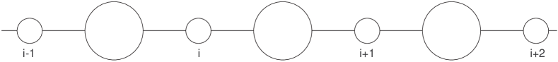
Figure 1: The model for one-dimensional ionic conductor. Large circles denote heavy ionic groups while the small ones denote light movable ions.

3 Exact diagonalization technique

We calculate the spectral densities of one-dimensional ionic Pauli conductor using exact diagonalization technique. For the chain of $N$ sites, we introduce the many-particle states

$$\mid n_{1,a}n_{1,b}\ldots n_{N,a}n_{N,b}\rangle.$$ (2)

The Hamiltonian matrix on the basis of these states is the matrix of the order $2^{N}\times 2^{N}$ and is constructed as follows:

$$H_{mn}=\sum\limits_{i=1}^{N}\left[t\left(H^{(1)}_{mn}+H^{(2)}_{mn}\right)+\widetilde{V}H^{(3)}_{mn}-\mu H^{(4)}_{mn}\right],$$ (3)

where

$$H^{(1)}_{mn} = \langle n_{1}\ldots|c^{+}_{i}c_{i+1}|n^{\prime}_{1}\ldots\rangle=\delta(n_{i}\!-\!n^{\prime}_{i}\!-\!1)\delta(n_{i+1}\!-\!n^{\prime}_{i+1}\!+\!1)$$

$$\times\prod\limits_{l\neq i;i+1}\delta(n_{l}\!-\!n^{\prime}_{l}),$$

$$H^{(2)}_{mn} = \langle n_{1}\ldots|c^{+}_{i+1}c_{i}|n^{\prime}_{1}\ldots\rangle=\delta(n_{i}\!-\!n^{\prime}_{i}\!+\!1)\delta(n_{i+1}\!-\!n^{\prime}_{i+1}\!-\!1)$$

$$\times\prod\limits_{l\neq i;i+1}\delta(n_{l}\!-\!n^{\prime}_{l}),$$

$$H^{(3)}_{mn} = \langle n_{1}\ldots|n_{i}n_{i+1}|n^{\prime}_{1}\ldots\rangle=\delta(n_{i}\!-\!1)\delta(n^{\prime}_{i}\!-\!1)\delta(n_{i+1}\!-\!1)$$

$$\times\delta(n^{\prime}_{i+1}\!-\!1)\prod\limits_{l\neq i;i+1}\delta(n_{l}\!-\!n^{\prime}_{l}),$$

$$H^{(4)}_{mn} = \langle n_{1}\ldots|n_{i}|n^{\prime}_{1}\ldots\rangle=\delta(n_{i}\!-\!1)\delta(n^{\prime}_{i}\!-\!1)\prod\limits_{l\neq i}\delta(n_{l}\!-\!n^{\prime}_{l}).$$

This matrix is diagonalized numerically

$$U^{-1}HU=\widetilde{H}=\sum\limits_{p}\lambda_{p}\widetilde{X}^{pp},$$ (4)

where $\lambda_{p}$ are eigenvalues of the Hamiltonian, $\widetilde{X}^{pp}$ are Hubbard-operators. The same transformation is applied to the creation and annihilation operators

$$U^{-1}c_{i}U=\sum\limits_{pq}A_{pq}\widetilde{X}^{pq}\,,\qquad U^{-1}c^{+}_{i}U=\sum\limits_{pq}A^{*}_{rs}\widetilde{X}^{rs}$$ (5)

which are required to construct one-particle Green’s function $\ll c_{i,a}|c^{+}_{i,a}\gg$ that contains information about one-particle energy spectrum of the system. For Pauli creation and annihilation operators, this Green’s function can be constructed in two ways, i.e., commutator Green’s function

$$\ll c_{i}(t)|c^{+}_{i}(t^{\prime})\gg=-{\rm i}\Theta(t-t^{\prime})\langle[c_{i}(t),c^{+}_{i}(t^{\prime})]\rangle$$ (6)

and anticommutator Green’s function

$$\ll c_{i}(t)|c^{+}_{i}(t^{\prime})\gg=-{\rm i}\Theta(t-t^{\prime})\langle\{c_{i}(t),c^{+}_{i}(t^{\prime})\}\rangle.$$ (7)

Imaginary part of these Green’s functions are one-particle spectral densities (also referred to as densities of states or DOS)

$$\rho(\omega) = -\frac{1}{\pi N}\sum\limits_{i=1}^{N}\textrm{Im}\ll c_{i,a}|c^{+}_{i,a}\gg$$ (8)

$$= -\frac{1}{\pi N}\sum\limits_{i=1}^{N}\textrm{Im}\left[\frac{1}{Z}\sum\limits_{pq}A_{pq}A^{*}_{pq}\frac{{\rm e}^{-\beta\lambda_{p}}-\eta{\rm e}^{-\beta\lambda_{q}}}{\omega-(\lambda_{q}-\lambda_{p})}\right],$$

where $Z=\sum_{p}{\rm e}^{-\beta\lambda_{p}}$. Spectral densities in (8), obtained from commutator $\eta=1$ (6) and anticommutator $\eta=-1$ (7) Green’s functions, respectively, exhibit a discrete structure, i.e., consist of several $\delta$-peaks due to the finite size of a cluster. Therefore, we apply the periodic boundary conditions to the cluster and introduce a small parameter $\Delta$ to broaden the $\delta$-peaks according to Lorentz distribution

$$\delta(\omega)\rightarrow\frac{1}{\pi}\frac{\Delta}{\omega^{2}+\Delta^{2}}\,.$$ (9)

4 Results and discussion

We perform calculations of one-particle spectral densities of one-dimensional ionic Pauli conductor (1) for the chain of ten sites ($N=10$) in periodic boundary conditions. To test the results we compare them with the exact solution obtained by means of fermionization procedure [14] in the absence of nearest neighbour interaction ($V=0$) for different values of chemical potential (figure 2). The redistribution of statistical weight with the change of chemical potential level can be observed, and a good level of agreement is achieved. The analysis of spectral densities is a way to distinguish the different states of an ionic subsystem and the corresponding conditions. In the case of half-filling, as we turn on the interaction starting with spectral density whose shape corresponds to SF state, we observe the development of the gap in the spectra (figure 3). A similar effect was found for ionic and proton conductors described by the similar models within the framework of Fermi statistics. It was connected with the splitting of spectra due to charge ordering with doubling of the lattice period [11, 12]. The detailed analysis of spectral densities of Fermi and Pauli models of ionic conductor can be found in [29]. So, here we have a transition from SF to CDW state. This transition was described analytically for $T=0$ in [30, 31]. We have investigated the case of $T\neq 0$ when this transition manifests itself as a crossover.

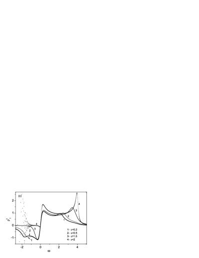
Figure 2: Commutator spectral densities of non-interacting ($V=0$) ionic Pauli conductor for different values of chemical potential (right figure, $\varepsilon=-\mu$) compared to exact results obtained in [14] via fermionization procedure (left figure, $\varepsilon=\varepsilon_{0}-\mu$). $t=1,T=0.2,\Delta=0.4$. Spectral density on the left figure is scaled to 2$\pi$, while on the right figure it is scaled to unity.

Figure 3: Commutator spectral density of ionic Pauli conductor for different values of nearest-neighbour interaction $V$ at half filling ($\mu=0$). $t=1,\,T=0.2,\,\Delta=0.4$.

The existence of a gap in the spectra which separates the bottom of the energy band from the chemical potential level is also the sign of the presence of homogenous MI state. The vanishing of the gap and the appearance of a negative branch points to the transition to SF-like state (see, for example, [32]). According to these criteria we analyze the spectral densities at different temperatures and values of interaction and build the corresponding diagrams of state (figure 4). The system is in MI homogenous state at high temperatures and far away from half-filling (at large $\delta$). As the temperature decreases or one comes closer to half-filled case, the system undergoes transition to SF-like state which corresponds to the appearance of the negative branch without any gap on the spectral density. At further temperature decrease and closer to half filling, we observe a transition to the state with the gap on the spectral density that corresponds to the CDW-ordering (the negative branch still exists). As the interaction strength $V$ increases, such a region becomes broader while the region of SF-like state becomes smaller. On the other hand, with the decrease of $V$, the CDW state diminishes and disappears at $V\approx t$. It should be mentioned that the sequence of states that the system is going through at the increase of mean occupancy $\delta$, corresponds to the phase diagram obtained in [30, 31, 33]. We have also performed a detailed analysis of the transition to SF-like state at different temperatures and values of interaction (figure 5). It is interesting that at weak interactions ($V<1$), the increase of interaction strength facilitates the formation of SF-like state while further increase of $V$ suppresses this transition. The shift of the curves that separate MI- and SF-states towards smaller values of $\delta$ with the increase of interaction strength that we have obtained is also observed on the phase diagrams obtained by other authors [30, 31].

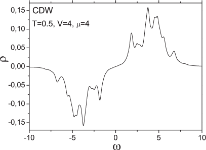
Figure 4: Diagrams of state for different interactions and the spectral densities for negative $\delta$ that correspond to CDW, SF and MI states. $t=1,\Delta=0.25$. $\delta=\langle n\rangle-1/2$ denotes the deviation from half-filling.

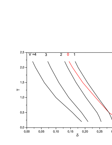
Figure 5: The curves that separate SF- and MI- states at different temperatures and values of interaction. SF-state is on the left hand side of the curves and below them. $t=1,\,\Delta=0.25$. $\delta=\langle n\rangle-1/2$ denotes the deviation from half-filling.

5 Conclusions

We have performed the analysis of diagrams of states of one-dimensional Pauli ionic conductor using an exact diagonalization technique. We have shown that the system undergoes transition from Mott insulator to superfluid-like state and then to CDW-sate. At weak interaction, the latter transition may vanish.

Спектральнi густини та дiаграми стану одновимiрного iонного провiдника Паулi I.В. Стасюк, О. Воробйов, Р.Я. Стецiв Iнститут фiзики конденсованих систем НАН України, вул. I. Свєнцiцького, 1, 79011 Львiв, Україна

References

- [1] Tomoyoze T., Seino M., J. Phys. Soc. of Japan, 1998, 67, 1667; doi:10.1143/JPSJ.67.1667.
-
[2]
Belushkin A.V., David V.I.F., Ibberson R.M., Shuvalov L.A.,
Acta Cryst. B, 1991, 47, 161;
doi:10.1107/S010876819001076X. - [3] Salejda W., Dzhavadov N.A., Phys. Stat. Sol. (b), 1990, 158, 119; doi:10.1002/pssb.2221580111.
- [4] Salejda W., Dzhavadov N.A., Phys. Stat. Sol. (b), 1990, 158, 475; doi:10.1002/pssb.2221580208.
-
[5]
Stasyuk I.V., Pavlenko N., Hilczer B., Phase Transitions,
1997, 62, 135;
doi:10.1080/01411599708220065. - [6] Pavlenko N.I., Phys. Rev. B, 2000, 61, 4988; doi:10.1103/PhysRevB.61.4988.
-
[7]
Krasnogolovets V.V., Tomchuk P.M.,
Phys. Stat. Sol. (b), 1985, 130, 807;
doi:10.1002/pssb.2221300247. -
[8]
Stasyuk I., Vorobyov O., Hilczer B.,
Solid Sate Ionics, 2001, 145, 211;
doi:10.1016/S0167-2738(01)00960-2. - [9] Stasyuk I.V., Vorobyov O., Condens. Matter Phys., 2003, 6, 43.
- [10] Stasyuk I.V., Vorobyov O., Integrated Ferroelectrics, 2004, 63, 215; doi:10.1080/10584580490459567.
- [11] Stasyuk I.V., Vorobyov O., Phase Transitions, 2007, 80, 63; doi:10.1080/01411590701315443.
- [12] Stasyuk I.V., Vorobyov O., Ferroelectrics, 2008, 376, 64; doi:10.1080/00150190802440765.
- [13] Mahan G.D., Phys. Rev. B, 1976, 14, 780; doi:10.1103/PhysRevB.14.780.
- [14] Stasyuk I.V., Dulepa I.R., Condens. Matter Phys., 2007, 10, 259.
- [15] Stasyuk I.V., Dulepa I.R., J. Phys. Stud., 2009, 13, 2701.
-
[16]
Micnas R., Ranninger J., Robaszkiewicz S.,
Rev. Mod. Phys., 1990, 62, 113;
doi:10.1103/RevModPhys.62.113. - [17] Mysakovych T.S., Krasnov V.O., Stasyuk I.V., Condens. Matter Phys., 2008, 11, 663.
- [18] Stasyuk I.V., Mysakovych T.S., Condens. Matter Phys., 2009, 12, 539.
- [19] Batrouni G.G., Scalettar R.T., Phys. Rev. B, 1992, 46, 9051; doi:10.1103/PhysRevB.46.9051.
- [20] Micnas R., Robaszkiewicz S., Phys. Rev. B, 1992, 45, 9900; doi:10.1103/PhysRevB.45.9900.
- [21] Batrouni G.G., Scalettar R.T., Phys. Rev. Lett., 2000, 84, 1599; doi:10.1103/PhysRevLett.84.1599.
- [22] Bernardet K., Batrouni G.G., Meunier J.-L., Schmid G., Troyer M., Dorneich A., Phys. Rev. B, 2002, 65, 104519; doi:10.1103/PhysRevB.65.104519.
-
[23]
Bernardet K., Batrouni G.G., Troyer M.,
Phys. Rev. B, 2002, 66, 054520;
doi:10.1103/PhysRevB.66.054520. -
[24]
Schmid G., Todo S., Troyer M., Dorneich A.,
Phys. Rev. Lett., 2002, 88, 167208;
doi:10.1103/PhysRevLett.88.167208. -
[25]
Vlaming R., Uhrig G.S., Vollhardt D.,
J. Phys. Cond. Matt. 1992, 4, 7773;
doi:10.1088/0953-8984/4/38/010. - [26] Lorenz B., Phys. Stat. Sol. (b) 1980, 101, 297; doi:10.1002/pssb.2221010131.
- [27] Stasyuk I.V., Ivankiv O.L., Pavlenko N.I., J. Phys. Stud., 1997, 1, 418.
-
[28]
Niyaz P., Scalettar R.T., Fong C.Y., Batrouni G.G.,
Phys. Rev. B, 1994, 50, 362;
doi:10.1103/PhysRevB.50.362. - [29] Vorobyov O., Stetsiv R.Ya., AIP Conference Proceedings 1198, Subseries: Mathematical and Statistical Physics, 2009, 204; doi:10.1063/1.3284416.
- [30] Khner T.D., White S.R., Monien H., Phys. Rev. B, 2000, 61, 12474; doi:10.1103/PhysRevB.61.12474.
- [31] Hen I., Rigol M., Phys. Rev. B, 2009, 80, 134508; doi:10.1103/PhysRevB.80.134508.
- [32] Menotti C., Trivedi N., Phys. Rev. B, 2008, 77, 235120; doi:10.1103/PhysRevB.77.235120.
- [33] Hen I., Iskin M., Rigol M., Phys. Rev. B, 2010, 81, 064503; doi:10.1103/PhysRevB.81.064503.