Fermi surface reconstruction in strongly correlated Fermi systems as a first order phase transition

Abstract

A quantum phase transition in strongly correlated Fermi systems beyond the topological quantum critical point is studied within the Fermi liquid approach. The transition occurs between two topologically equivalent states, each with three sheets of the Fermi surface. One of these states possesses a quasiparticle halo in the quasiparticle momentum distribution $n(p)$, while the other, the hole pocket. The transition is found to be of the first order with respect to both the coupling constant $g$ and the temperature $T$. The phase diagram of the system in the vicinity of this transition is constructed.

Low temperature quantum phase transitions in strongly correlated Fermi systems is one of hot topics in the condensed matter physics in the last decade. Variation of external parameters (pressure, density, magnetic field) allows one to shift the transition temperature to zero and to obtain the quantum critical point, which is associated with divergence of the effective mass $M^{*}$. In the vicinity of this point, low temperature properties of the system possess non-Fermi-liquid character, i.e. they are not described within the conventional Landau theory of Fermi liquid.

At present, experimental information on the quantum critical point is available only for three types of strongly correlated Fermi systems: i) the inversion layer in MOSFET silicon transistors in which electrons form a two-dimensional (2D) liquid, Shashkin-PRB-2002 ; Pudalov-PRL-2002 ii) films of ³He atoms on various substrates, Godfrin-JLT-1998 ; Saunders-Science-2007 iii) metals with heavy fermions. Oeschler-PB-2008 ; Gegenwart-NP-2008

In nonsuperfluid homogeneous and isotropic Fermi systems, which will be considered in this work, the ratio of the effective mass $M^{*}$ to the bare one $M$ reads

$${M\over M^{*}}=z\left[1+\left({\partial\Sigma(p,\varepsilon)\over\partial\epsilon^{0}_{p}}\right)_{0}\right]\ ,$$ (1)

where $\epsilon^{0}_{p}=p^{2}/2M-\mu$, $\mu$ is the chemical potential, $\Sigma$ is the mass operator, and the quasiparticle weight $z$ in a single particle state is given by $z=[1-\left(\partial\Sigma(p,\varepsilon)/\partial\varepsilon\right)_{0}]^{-1}$ (index $0$ means evaluation of the derivative on the Fermi surface). The formula (1) allows one to consider two scenarios of the quantum critical point. The collective scenario is build on a supposition that energy dependence of the mass operator prevails over its momentum dependence due to exchange by critical fluctuations in the vicinity of collapse point of the respective collective mode, and leads to vanishing of the quasiparticle weight $z$ and, hence, to divergence of the effective mass $M^{*}$ just at that point. Gegenwart-NP-2008 ; Hertz-PRB-1976 ; Millis-PRB-1993 ; Coleman-JPCM-2001 The topological scenario of the critical point assumes $z$-factor to be finite at that point, however dominating momentum dependence of the mass operator results in the change of the Fermi surface topology. KS-JETPL-1990 ; Volovik-JETPL-1991 ; Nozieres-1992 ; Khodel-JETPL-2007 ; KCZ-PRB-2008 The reader can find comparison of these two scenarious in Refs. Khodel-JETPL-2007, ; KCZ-PRB-2008, . In this paper, we consider the topological scenario of the quantum critical point.

In this connection, it is worth to note that in accordance with topological classification Volovik-book-2007 of ground states of fermionic systems, the basic classes differ by topological dimension ${\cal D}$ of the manifold of nodes of the single-particle spectrum $\epsilon(p)$ measured from the chemical potential. Within the same class, we will distinguish states by a number of connected sheets of that manifold. All transitions between ground states which belong to different topological classes or transitions between states with different topology in the same class are quantum phase transitions occurring at $T=0$. Conventional nonsuperfluid homogeneous and isotropic Fermi liquid at $T=0$ with quasiparticle momentum distribution $n_{\mbox{\scriptsize FL}}(p)=\theta(p_{F}-p)$ belongs to the class for which the dimension ${\cal D}$ of the manifold of nodes is less by unity than the dimension of the system itself, and this manifold is a single connected sheet, i.e. the Fermi surface.

Violation of the necessary stability condition for Landau quasiparticle ground state with the momentum distribution $n_{\mbox{\scriptsize FL}}(p)$ serves a signal for its topological reconstruction. This stability condition

$$\delta E=2\int\epsilon(p,[n_{\mbox{\scriptsize FL}}(p)])\,\delta n_{\mbox{\scriptsize FL}}({\bf p})\,d\upsilon>0$$ (2)

demands positivity of variation of the ground state energy $E$ for any admissible variation $\delta n_{\mbox{\scriptsize FL}}({\bf p})$ which satisfies the condition

$$2\int\delta n_{\mbox{\scriptsize FL}}({\bf p})\,d\upsilon=0\ .$$ (3)

In Eqs. (2) and (3), $d\upsilon$ denotes an elementary volume of the momentum space, and a factor of two means summation over two spin projections. The distribution $n_{\mbox{\scriptsize FL}}(p)$ satisfies the necessary condition (2) provided the single-particle spectrum $\epsilon(p,[n_{\mbox{\scriptsize FL}}(p)])$ vanishes only at $p=p_{F}$. In weakly and moderately correlated systems this is true. However, in process of correlations strengthening with the change of external parameters, new nodes of the function $\epsilon(p,[n_{\mbox{\scriptsize FL}}(p)])$ can appear and the condition (2) is then violated. KS-JETPL-1990 ; Volovik-JETPL-1991 ; Nozieres-1992

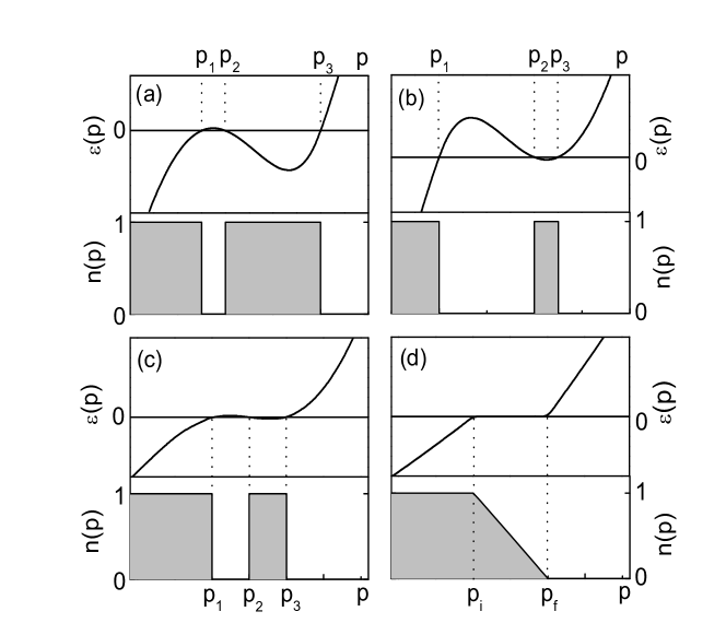
Figure 1: Single-particle spectrum and momentum distribution of quasiparticles: illustration of topological reconstruction scenarios. Panel (a): hole pocket, panel (b): quasiparticle halo, panel (c): symmetrical three-connected distribution, panel (d): fermion condensate.

Two scenarios of topological reconstruction of the momentum distribution $n_{\mbox{\scriptsize FL}}(p)$ resulting from this violation are known: i) reconstruction within the same topological class, i.e. with no change of the dimension ${\cal D}$ but with change of the number of connected sheets of the Fermi surface, Frohlich-PR-1950 ; Vary-PRC-1979 ; Zabolitsky-PRC-1979 ; Aguilera-PRC-1982 ; ZB-JETP-1998 ; ZB-JPCM-1999 ; Shaginyan-JETPL-1998 ; Schofield-PRB-2006 ii) reconstruction with transition to another topological class, i.e. with change of the dimension ${\cal D}$. KS-JETPL-1990 ; Volovik-JETPL-1991 ; Nozieres-1992 When new nodes of the spectrum appear on the same side from the Fermi surface, the distribution $n_{\mbox{\scriptsize FL}}(p)$ is rearranged to asymmetric three-connected momentum distribution which is schematically shown in the panels (a) and (b) of Fig. 1. If the nodes $p_{1}$, $p_{2}$, $p_{3}$ are arranged in such a way that $|p_{1}-p_{2}|\ll|p_{2}-p_{3}|$ the distribution has a form of the hole pocket in the filled sphere (we refer to this state as to ${\cal H}$-state), while if $|p_{1}-p_{2}|\gg|p_{2}-p_{3}|$, one deals with the quasiparticle halo (${\cal P}$-state). Such reconstruction results in no change of the topological dimension ${\cal D}$, while the number of connected sheets of the Fermi surface appears to equal three. If new nodes of the spectrum emerge to both sides of the Fermi surface, then together with formation of symmetrical three-connected Fermi surface ZB-JETP-1998 ; ZB-JPCM-1999 ; Shaginyan-JETPL-1998 (see panel (c) of Fig. 1), essentially different scenario of rearrangement of Landau state is possible, fermion condensation, KS-JETPL-1990 ; Volovik-JETPL-1991 ; Nozieres-1992 shown in the panel (d) of Fig. 1. In this scenario the quasiparticle momentum distribution gradually drops within the interval $p_{i}<p<p_{f}$, and the spectrum $\epsilon(p)$ identically vanishes within this interval. Hence the state with fermion condensate turns out to belong to the class with the topological dimension of manifold of nodes ${\cal D}$ coinciding with dimension of the system. The fermion condensate, revealed and studied in details about 20 years ago, KS-JETPL-1990 ; Volovik-JETPL-1991 ; Nozieres-1992 acquires a new life in these days in a form of topologically protected flat bands, i.e. dispersionless branches of the single-particle spectrum with exactly zero energy. Volovik-1012-0905 ; Brydon-1104-2257 Particularly, possibility of existence of surface states with flat band is intensively discussed, Volovik-1012-0905 ; Brydon-1104-2257 ; Schnyder-1011-1438 ; Volovik-1103-2033 which may be superconducting with high transition temperature. Volovik-1103-2033

In this paper, we consider the scenario of the topological reconstruction with formation of three-connected Fermi surface. We will show that in a topologically rearranged system, the first order transition between ${\cal P}$- and ${\cal H}$-states may occur.

We focus now on the scenario of topological transition in which only regions adjacent to the Fermi surface are involved. Results of microscopic calculations for 2D liquid ³He Krotscheck-PRL-2003 and for low-density 2D electron gas BZ-JETPL-2005 indicate this way of topological reconstruction in these systems. For evaluation of the single-particle spectrum $\epsilon(p)$ and momentum distribution of quasiparticles $n(p)$ we use the Fermi-liquid relation Landau-JETP-1956 ; Landau-JETP-1958 ; LL-Stat-IX ; Trio

$${\partial\epsilon(p)\over\partial{\bf p}}={{\bf p}\over M}+\int\!f({\bf p},{\bf p_{1}})\,{\partial n(p_{1})\over\partial{\bf p_{1}}}\,d\upsilon_{1}\ ,$$ (4)

in which $n(p)=\theta(-\epsilon(p))$ and the quasiparticle interaction $f({\bf p},{\bf p_{1}})$ in the Fermi liquid theory is supposed to be known function of momenta. The formula (4) represents the nonlinear integro-differential equation for the single-particle spectrum $\epsilon(p)$. Any numerical algorithm of its solution requires use of regularization procedure. This is finite temperature that plays a role of a natural physical regularizer. Indeed, making use of the Fermi-Dirac relation between momentum distribution and spectrum

$$n(p,T)=\left[1+e^{\epsilon(p)/T}\right]^{-1}$$ (5)

allows one to solve Eq. (4) by standard iterative algorithm.

We analyze the topological reconstruction in 2D Fermi system with a quasiparticle interaction function

$$f({\bf p},{\bf p_{1}})=-g{\pi\over M}{1\over(({\bf p}-{\bf p_{1}})^{2}/q_{0}^{2}-1)^{2}+\beta^{2}}\ ,$$ (6)

with $q_{0}\simeq 2p_{F}$, $\beta$=0.14, which enables one to reproduce adequately microscopic calculations BZ-JETPL-2005 of single-particle spectra of 2D electronic gas at $T=0$ on the Fermi-liquid side from the quantum critical point. Since the interaction function depends on the difference ${\bf p}-{\bf p}_{1}$, Eq. (4) is integrated to the form

$$\epsilon(p)={p^{2}\over 2M}-\mu+\int\!f({\bf p},{\bf p_{1}})\,n(p_{1})\,d\upsilon_{1}\ ,$$ (7)

in which the chemical potential $\mu$ is obtained from the normalization condition

$$2\int n(p)\,d\upsilon=\rho\ .$$ (8)

Single-particle spectrum $\epsilon(p)$ and quasiparticle momentum distribution are evaluated by self-consistent solution of Eqs. (5), (7) and (8). Rearrangement of the ground state of the considered system with increase of the interaction constant $g$ is shown in Fig. 2. Calculations are performed at $T=10^{-5}\varepsilon_{F}^{0}$ modeling zero temperature. Irregularity of the spectrum at $p>p_{F}$ distinguished in the panel (a) of this Figure is developed to its nonmonotonous behavior which, as $g$ reaches $g_{b}=0.18$, results in the bifurcation in the equation $\epsilon(p)=0$ at $p=p_{b}>p_{F}$ (see panel (b)) and then, to the topological reconstruction with formation of the ${\cal P}$-state (panel (c)).

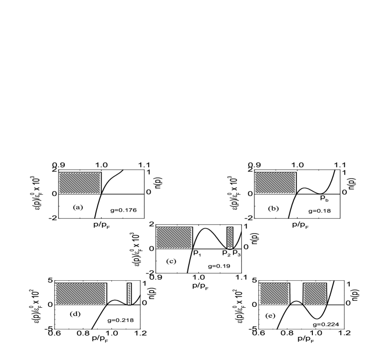
Figure 2: Single-particle spectra $\epsilon(p)$ and quasiparticle momentum distributions $n(p)$ evaluated at $T=10^{-5}$ in units of $\varepsilon_{F}^{0}=p_{F}^{2}/2M$ for the model with the interaction (6) with $q_{0}=2p_{F}$ for different values of the interaction constant $g$: 0.176 (panel (a)), 0.180 (panel (b)), 0.190 (panel (c)), 0.218 (panel (d)) and 0.224 (panel (e)).

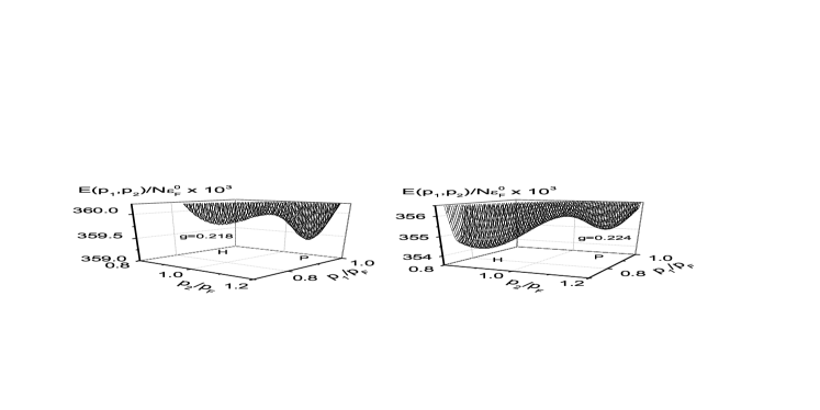
Figure 3: Energy per one particle as a function of $p_{1}$ and $p_{2}$ evaluated at $T=0$ for $q_{0}=2\,p_{F}$.

The three-connected momentum distribution at zero temperature $n_{3}(p)=\theta(p_{1}-p)-\theta(p_{2}-p)+\theta(p_{3}-p)$ is determined in the functional space by two independent parameters, the third one being obtained from the relation

$$p_{1}^{2}-p_{2}^{2}+p_{3}^{2}=p_{F}^{2}\ ,$$ (9)

following from the normalization condition (8). This implies that the energy functional of the system

$$E[n]=2\int\frac{p^{2}}{2M}n({\bf p})\,d\upsilon+\int f({\bf p},{\bf p_{1}})n({\bf p})n({\bf p_{1}})\,d\upsilon d\upsilon_{1}$$ (10)

considered within the class of distributions $n_{3}(p)$ is just a function of two variables, say, $p_{1}$ and $p_{2}$. Evaluation of the function $E(p_{1},p_{2})$ indicates that the momentum distribution $n(p)$ obtained by self-consistent solution of Eqs. (5), (7), (8) and shown in the panel (c) of Fig. 2 corresponds to the global minimum of this function. There is no other local minimum of $E(p_{1},p_{2})$ just beyond the topological transition point. However, the situation changes with increasing coupling constant, namely, a new minimum appears at $g\simeq 0.21$. The relief of the function $E(p_{1},p_{2})$ at $g=0.218$ is shown in the left panel of Fig. 3. The deep minimum at $p_{2}>p_{F}$ corresponds to the ground ${\cal P}$-state, the quasiparticle momentum distribution and the spectrum of which are shown in the panel (d) of Fig. 2. The shallow minimum at $p_{2}<p_{F}$ corresponds to the metastable ${\cal H}$-state which is obtained by solving of the set of Eqs. (5), (7), (8) provided the iteration procedure is started from a state inside the shallow well With further increasing of the coupling constant $g$, the ${\cal H}$-state minimum lowers with respect to the ${\cal P}$-state minimum, and both minima equalize at $g=0.22$. The first-order transition from the ${\cal P}$-state to the ${\cal H}$-state occurs at this point, the latter state becomes the ground one at $g>0.22$. This is demonstrated in the right panel of Fig. 3 where the relief $E(p_{1},p_{2})$ at $g=0.224$ is drawn. The deep minimum corresponds to the ${\cal H}$-state shown in the panel (c) of Fig. 2. As follows from calculations made up to $g=0.26$, the ${\cal P}$-state keeps on existing as a metastable one.

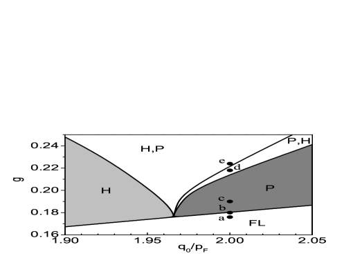
Figure 4: Phase diagram in $(q_{0},g)$ variables. Capital letters denote the state occupying corresponding part of the diagram. Two letters mean that the first state is the ground state, while the second one is metastable.

Figure 5: Quasiparticle momentum distributions and single-particle spectra evaluated in the model (11). Panel (a) shows unstable Landau state, panel (b) demonstrates the ${\cal H}$-state, panel (c) — the ${\cal P}$-state. Single-particle spectrum for the Landau state $\epsilon(p,[n_{\mbox{\scriptsize FL}}])$ shifted by the respective difference of chemical potentials is shown for comparison in panels (b) and (c) by dashed lines.

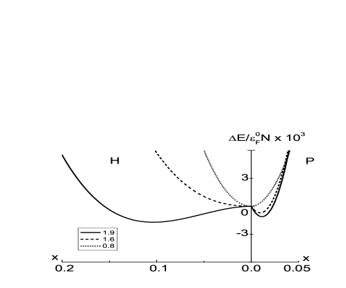
Figure 6: Energies per one particle in units of $\varepsilon^{0}_{F}$ evaluated for the ${\cal H}$-state (left part of the figure) and the ${\cal P}$-state (right part) at three values of the constant $f$.

Analysis of metamorphoses of solutions of Eqs. (5), (7), (8) with variation of both the coupling constant $g$ and the wave vector $q_{0}$ allows one to build the phase diagram of the system in these variables which is shown in Fig. 4. At $q_{0}>1.96\,p_{F}$, the diagram is arranged similarly to the one considered above for $q_{0}=2\,p_{F}$. Five points on it correspond to five solutions shown in Fig. 2. Arrangement of the phase diagram at $q_{0}<1.96\,p_{F}$ is different, namely, the three-connected ${\cal H}$-state emerges just beyond the point of the topological transition and remains the ground state while the metastable ${\cal P}$-state appears with increasing $g$.

It is worth noting that the first-order transition under consideration is not inherent in 2D systems only. Analysis for 3D systems shows that an analogous transition occurs in 3D as well.

Why the considered set of equations possesses simultaneously two solutions at fixed parameters, can be understood with a help of a simplified model with $\delta$-function quasiparticle interaction. 3D system is somewhat more convenient for this purpose than 2D one since all calculations can be done analytically for the 3D case. For the model interaction

$$f(q)=-f{8\pi^{2}p_{F}\over M}\delta({\bf q}^{2}-q_{0}^{2})$$ (11)

with $q_{0}\simeq 2\,p_{F}$, the state with quasiparticle momentum distribution $n_{3}(p)$ at $T=0$ has the spectrum

$$\epsilon(p;[n_{3}])={p^{2}\over 2M}-\mu$$ (12)

$$+f{p_{F}\over 2Mp}\sum_{k=1}^{3}(-1)^{k+1}[(p{-}q_{0})^{2}{-}p_{k}^{2}]\,\theta(p{+}p_{k}{-}q_{0}).\qquad$$

Single-particle spectra evaluated with use of Eq. (12) with $q_{0}=2\,p_{F}$, $f=2.0$ are displayed in Fig. 5. The spectrum $\epsilon(p;[n_{\mbox{\scriptsize FL}}])$ given by an account of the only term in the sum in (12) with the boundary momentum $p_{F}$ is shown in the panel (a). Due to $\theta$-function on the r.h.s. of Eq. (12), the spectrum possesses a kink and changes its behavior at the point $p^{(1)}=q_{0}-p_{F}=p_{F}$. The necessary condition (2) for stability of the Landau state with the quasiparticle distribution $n_{\mbox{\scriptsize FL}}(p)$ is, evidently, violated. The spectra $\epsilon(p;[n_{3}])$ shown by solid lines on panels (b) and (c) possesses three kinks. If $p_{2}<p_{F}$, the second kink is placed at the point $p^{(2)}=q_{0}-p_{2}$ lying to the right of $p_{F}$. In this case tuning of the chemical potential to the condition of conservation of the quasiparticle number gives rise self-consistently to the ${\cal H}$-state. Such state with the nodes $p_{1}=0.82\,p_{F}$, $p_{2}=0.96\,p_{F}$, $p_{3}=1.1\,p_{F}$ is shown on panel (b) of Fig. 5 together with the spectrum for the Landau state shifted for convenience by the difference of the chemical potentials. In case $p_{2}>p_{F}$, the point of the second kink is placed to the left of $p_{F}$, and then tuning of the chemical potential gives rise to the ${\cal P}$-state. The spectrum of this state with the nodes $p_{1}=0.97\,p_{F}$, $p_{2}=1.16\,p_{F}$, $p_{3}=1.18\,p_{F}$ is shown on panel (c) together with shifted spectrum $\epsilon(p;[n_{\mbox{\scriptsize FL}}])$.

To elucidate which of the two states, ${\cal H}$ or ${\cal P}$, proves to be the ground one, we evaluate the energies of these states. Dimensionless energy of the tree-connected state per one particle ${\cal E}=\Delta E/\varepsilon_{F}^{0}N$ measured from the energy of the Landau state is given as follows

$${\cal E}=\frac{3}{5p_{F}^{5}}\left(p_{1}^{5}-p_{2}^{5}+p_{3}^{5}-p_{F}^{5}\right)$$ (13)

$$-\frac{2fq_{0}}{p_{F}}\left(S(q_{0};[n_{3}])-S(q_{0};[n_{\mbox{\scriptsize FL}}])\right).\qquad$$

Upon not difficult but cumbersome algebra, the structure function

$$S(q;[n])=\frac{2}{\rho}\int n({\bf p}+{\bf q})n({\bf p})\frac{d^{3}{\bf p}}{(2\pi)^{3}}$$ (14)

is evaluated analytically. Excluding, say, the variable $p_{3}$, one then arrives at the energy as a function of two variables, $p_{1}$ and $p_{2}$. The condition of its extremum allows one to express $p_{2}$ via $p_{1}$ and reduce the energy to the function of a single variable $p_{1}$. Let $q_{0}=2\,p_{F}$, we introduce then a new convenient variable $x=1-p_{1}/p_{F}$. For small values of $x$, the energy of the ${\cal P}$-state equals

$${\cal E}_{\cal P}(x)=-a_{\cal P}\,(\delta_{\cal P}^{2}-\frac{3}{4}\delta_{\cal P}^{3})\,\theta(\delta_{\cal P})\,x+b_{\cal P}\,x^{2},$$ (15)

where $\delta_{\cal P}=f-f_{\cal P}^{c}$ is an excess of the coupling constant $f$ over the critical value $f_{\cal P}^{c}=1$ corresponding to the topological transition from the Landau state to the ${\cal P}$-state, $a_{\cal P}=3/4$, $b_{\cal P}=6$. For the ${\cal H}$-state, one analogously obtains

$${\cal E}_{\cal H}(x)=-a_{\cal H}\,\delta_{\cal H}\,x^{2}+b_{\cal H}\,x^{3},$$ (16)

where $\delta_{\cal H}=f-f_{\cal H}^{c}$, $f_{\cal H}^{c}=1+1/\sqrt{2}$ is a critical value of the constant at which the metastable ${\cal H}$-state emerges, $a_{\cal H}=6(\sqrt{2}-1)$, $b_{\cal H}=9/2-\sqrt{2}$. Expressions (15) and (16), formally applicable in the vicinity of the respective critical constants, qualitatively describe behavior of the energies of ${\cal P}$- and ${\cal H}$-phases far from $f_{\cal P}^{c}$ and $f_{\cal H}^{c}$ as well.

As long as $\delta_{\cal P}<0$, the linear in $x$ term in the energy excess of the ${\cal P}$-state over the Landau state equals zero and ${\cal E}_{\cal P}(x)=b_{\cal P}\,x^{2}>0$. For such values of the coupling constant, $\delta_{\cal H}$ is also negative and, hence, both terms in ${\cal E}_{\cal H}(x)$ are positive. Therefore, the Landau state with the quasiparticle distribution $n_{\mbox{\scriptsize FL}}(p)$ is the ground state. The functions ${\cal E}_{\cal P}(x)$ and ${\cal E}_{\cal H}(x)$ at $f<f_{\cal P}^{c}$ are shown by dotted lines in Fig. 6. At $\delta_{\cal P}>0$, linear in $x$ term with minus sign emerges in ${\cal E}_{\cal P}(x)$. As a result, the ${\cal P}$-state wins the contest against the Landau state. Thus, the second order topological transitions occurs at $f=f_{\cal P}^{c}$, namely, the three-connected ${\cal P}$-state with the quasiparticle halo appears to be the ground state. The energy ${\cal E}_{\cal H}(x)$ remains a monotonically growing function of $x$ as long as $\delta_{\cal H}<0$. Both energy curves at the constant $f=1.6$ corresponding to the case $f_{\cal P}^{c}<f<f_{\cal H}^{c}$ are shown by dashed lines in Fig. 6. As soon as $f$ exceeds $f_{\cal H}^{c}$, the coefficient near the quadratic term in the function ${\cal E}_{\cal H}(x)$ changes the sign and the function acquires the minimum, i.e. the metastable ${\cal H}$-state appears. When with incresing $f$, this minimum shown by a solid curve in the left part of Fig. 6 becomes deeper than the minimum of the right solid curve ${\cal E}_{\cal P}(x)$, the three-connected ${\cal H}$-state with the hole pocket, topologically equivalent to the ${\cal P}$-state, becomes the ground state. The transition between the ${\cal P}$- and ${\cal H}$-states is first order.

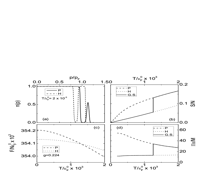
Figure 7: Panel (a): momentum distributions $n(p)$ for the ${\cal P}$- and the ${\cal H}$-states at $T=2\cdot 10^{-3}\varepsilon_{F}^{0}$. Entropy per one particle $S/N$ (panel (b)), free energy $F$ per one particle $F/N$ in units of $\varepsilon^{0}_{F}$ (panel (c)) and density of single-particle states $\Pi$ in units of $M/\pi$ (panel (d)) as functions of temperature $T$ in units of $\varepsilon^{0}_{F}$. Parameters $g=0.224$, $q_{0}=2\,p_{F}$ are used in the calculations.

We return now to the model of 2D electron gas with the quasiparticle interaction (6). The height of the energy barrier which, as seen in Fig. 3, is of order $10^{-3}\varepsilon^{0}_{F}$, determines the scale of temperature at which on can expect a transition between ${\cal H}$- and ${\cal P}$-states with increasing temperature. Such transition, indeed, occurs. This is caused by the fact that the quasiparticle halo is more narrow than the hole pocket, and hence, “melts” faster as temperature increases, what is demonstrated in panel (a) of Fig. 7. As a result, the entropy $S_{\cal P}(T)$ of the ${\cal P}$-state increases faster with heating than the entropy $S_{\cal H}(T)$ (see panel (b)), while the free energy $F_{\cal P}(T)$ decreases more rapidly than $F_{\cal H}(T)$ (panel (c)). Both minima equalize at $T_{1}\simeq 1.2\cdot 10^{-3}\varepsilon^{0}_{F}$, and the first order transition occurs from the ${\cal H}$-state to the ${\cal P}$-state. The entropy and the density of states undergo a jump at $T=T_{1}$ (see panels (b) and (d)). The considered transition may have relation to observed low-temperature anomalies in specific heat and magnetic susceptibility of metals with heavy fermions. Oeschler-PB-2008 ; Klingner-PRB-2011

In conclusion, we analyzed the reconstruction of the Fermi surface of the uniform Fermi system with increasing coupling constant of the quasiparticle interaction and found that the topological transition, in which two new connected sheets of the Fermi surface appear, is followed by the transition between two topologically equivalent states. The Fermi surface of both these states consists of three connected sheets, but one of these states, the ${\cal P}$-state, possesses a structure of the quasiparticle halo, while the second one, the ${\cal H}$-state, that of the hole pocket. The transition from the ${\cal P}$-state to the ${\cal H}$-state is of the first order with respect to the coupling constant $g$. As the temperature $T$ increases, the inverse first order transition from the ${\cal H}$-state to the ${\cal P}$-state occurs due to more rapid “melting” of the narrow quasiparticle halo and more rapid increase of its entropy with heating than increase of the entropy of the hole pocket.

We thank V. A. Khodel and G. E. Volovik for fruitful discussions. This research was supported by Grants No. 2.1.1/4540 and NS-7235.2010.2 from the Russian Ministry of Education and Science, and by Grant No. 09-02-01284 from the Russian Foundation for Basic Research.

References

- (1) A. A. Shashkin, S. V. Kravchenko, V. T. Dolgopolov et al., Phys. Rev. B 66, 073303 (2002).
- (2) V. M. Pudalov, M E. Gershenson, H. Kojima, et al., et al., Phys. Rev. Lett. 88, 196404 (2002).
- (3) C. Bäuerle, Yu. M. Bun’kov, A. S. Chen, S. N. Fisher, and H. Godfrin, J. Low Temp. 110, 333 (1998).
- (4) M. Neumann, J. Nyeki, B. P. Cowan, and J. Saunders, Science 317, 1356 (2007).
- (5) N. Oeschler, S. Yartmann, A. P. Pikul, C. Krellner, C. Geibel, F. Steglich, Physica B 403, 1254 (2008).
- (6) P. Gegenwart, Q. Si, F. Steglich, Nature Phys. 4, 186 (2008).
- (7) J. A. Hertz, Phys. Rev. B 14, 1165 (1976).
- (8) A. J. Millis, Phys. Rev. B 48, 7183 (1993).
- (9) P. Coleman, C. Pepin, Q. Si, and R. Ramazashvili, J. Phys.: Condens. Matter 13, R723 (2001).
- (10) V. A. Khodel and V. R. Shaginyan, JETP Lett. 51, 553 (1990).
- (11) G. E. Volovik, JETP Lett. 53, 222 (1991).
- (12) P. Nozières, J. Phys. I France 2, 443 (1992).
- (13) V. A. Khodel, JETP Letters 86, 721 (2007).
- (14) V. A. Khodel, J. W. Clark, M. V. Zverev, Phys. Rev. B 78, 075120 (2008).
- (15) G. E. Volovik, Springer Lecture Notes in Physics 718, 31 (2007).
- (16) H. Fröhlich, Phys. Rev. 79, 845 (1950).
- (17) M. de Llano, J. P. Vary, Phys. Rev. C 19, 1083 (1979).
- (18) M. de Llano, A. Plastino, J. G. Zabolitsky, Phys. Rev. C 20, 2418 (1979).
- (19) V. C. Aguilera-Navarro, M. De Llano, J. W. Clark, A. Plastino, Phys. Rev. C 25, 560 (1982).
- (20) M. V. Zverev and M. Baldo, JETP 87, 1129 (1998).
- (21) M. V. Zverev, M. Baldo, J. Phys.: Condens. Matter 11, 2059 (1999).
- (22) S. A. Artamonov, V. R. Shaginyan, and Yu. G. Pogorelov, JETP Lett. 68, 942 (1998).
- (23) J. Quintanilla, A. J. Schofield, Phys. Rev. B 74, 115126 (2006).
- (24) T. T. Heikkilä, N. B. Kopnin and G. E. Volovik, arXiv:1012.0905.
- (25) P. M. R. Brydon, A. P. Schnyder, C. Timm, arXiv:1104.2257.
- (26) A. P. Schnyder and S. Ryu, arXiv:1011.1438.
- (27) N. B. Kopnin, T. T. Heikkilä and G. E. Volovik, arXiv:1103.2033.
- (28) J. Boronat, J. Casulleras, V. Grau, E. Krotscheck, and J. Springer, Phys. Rev. Lett. 91, 085302, 2003.
- (29) V. V. Borisov and M. V. Zverev, JETP Letters 81, 503 (2005).
- (30) L. D. Landau, Sov. Phys. JETP 30, 1058 (1956).
- (31) L. D. Landau, Sov. Phys. JETP 35, 97 (1958).
- (32) L. D. Landau and E. M. Lifshitz, Statistical Physics, Vol. 2 (Pergamon Press, Oxford, 1980).
- (33) A. A. Abrikosov, L. P. Gor’kov, and I. E. Dzyaloshinski, Methods of Quantum Field Theory in Statistical Physics, (Prentice-Hall, London) 1963.
- (34) C. Klingner, C. Krellner, M. Brando, et al., Phys. Rev. B 83, 144405 (2011).