Thermalization and Quantum Correlations in Exactly Solvable Models

Abstract

The generalized Gibbs ensemble introduced for describing few body correlations in exactly solvable systems following a quantum quench is related to the nonergodic way in which operators sample, in the limit of infinite time after the quench, the quantum correlations present in the initial state. The nonergodicity of the correlations is thus shown analytically to imply the equivalence with the generalized Gibbs ensemble for quantum Ising and XX spin chains as well as for the Luttinger model the thermodynamic limit, and for a broad class of initial states and correlation functions of both local and nonlocal operators.

I Introduction

Following a number of groundbreaking experiments with ultracold atomic systems Weiss ; Schmiedmayer ; Bloch , the problem of thermalization of exactly solvable quantum many-body systems has attracted a great deal of attention Rigol_gge ; Cazalilla ; attention . This is because it relates to fairly fundamental questions, such as the emergence of thermodynamics in isolated systems prepared in initial states that are not eigenstates of the Hamiltonian (i.e. systems undergoing a so-called ‘quantum quench’). The latter subject has deep ramifications, both in condensed matter physics CazalillaRigol ; Polkovnikovetal and cosmology PolkovnikovGritsev ; Polkovnikovetal . Moreover, this problem is also relevant to the ongoing efforts to build ‘quantum emulators’, that is, tunable quantum systems capable of accurately simulating the mathematical models of many body physics. In this regard, the problem of thermalization impacts on questions such like how much memory will the emulator retain of its initial conditions and whether the standard Gibbsian ensembles can be used to predict the outcome of the simulation CazalillaRigol ; Polkovnikovetal .

Interestingly, it was first conjectured by Rigol and coworkers Rigol_gge that the steady state of simple few-body observables of integrable systems following a quantum quench can be described by a generalized Gibbs ensemble (GGE). The density matrix of the GGE is obtained as the less biased guess Jaynes of the steady state given the constraints on the dynamics stemming from the existing set of non-trivial integrals of motion. Surprisingly, it was found that, in order to reproduce few body observables, only a subset of the order of $L$ (where $L$ is the system size) of simple integrals of motion is needed Rigol_gge .

Concerning the general applicability of the GGE, there has been also some debate Silva about the importance for thermalization of the locality of the operators in the basis of eigenmodes of the system. For the quantum Ising chain, it was recently shown analytically that correlation functions of nonlocal operators also thermalize to the GGE Calabrese_Ising . Similar results had been found earlier for the Luttinger Cazalilla and sine-Gordon models Iucci2 .

However, the reason why the GGE has been so successful in explaining the steady-state correlations in very diverse models has remained rather obscure. For local operators in certain integrable field theories, solid arguments in favor of the validity of the GGE have been put forward by Fioretto and Mussardo FiorettoMussardo . Furthermore, Cassidy and coworkers Cassidy recently introduced a generalization of the eigenstate thermalization hypothesis (ETH) ETH ; Rigol_ETH for integrable systems. Previously, the ETH has been successfully used to understand thermalization in non-integrable systems Rigol_ETH .

In this work, we describe a general method to demonstrate the applicability of the GGE in exactly solvable models for a general class of initial states. Our method does not require the explicit evaluation of correlation functions at asymptotically long times after the quench. Instead, it suffices to show that the asymptotic correlation functions of (either local or nonlocal) operators depend only on the expectation values of quasi-particle occupation operators in the initial state. This property, together with certain properties of the class of initial states considered in this work MCChung ; MingPeschel , allows to demonstrate that each eigenmode of the system is subject to a (mode) dependent effective temperature, the latter being nothing but a restatement of the GGE conjecture. This new point of view on the GGE also explains some of the less well understood aspects of the conjecture that have been briefly mentioned above. As a matter of fact, it explains why the only set of integrals of motion that are needed to construct the GGE correspond to the quasi-particle occupation operators. For the class of exactly solvable models discussed below, the latter are a minimal set of $L$ integrals of motion that entirely determine the asypmtotic correlations. The fact that the asymptotic correlation functions depend only on the expectation value of these non-trivial integrals of motion means that the system remembers much more information about its initial conditions than it is the case in systems exhibiting thermalization to a standard Gibbs ensemble. For the latter, only the expectation value of the energy and the Hamiltonian suffice to determine the effective temperature and chemical potential of the standard Gibbs ensemble describing thermal equilibrium of systems in the thermodynamic limit. The lack of relaxation of correlation functions to thermal equilibrium found in this work bears a strong resemblance with the nonergodicity of the magnetization in the XY model discussed several decades ago by McCoy McCoyII and Mazur Mazur (see Polkovnikovetal for a recent review of this result). Thus, we shall call this behavior of the asymptotic correlations ‘nonergodic’.

Our goal in this article will be to illustrate our method to demonstrate the applicability of the GGE by applying it to several models that have been previously analyzed either analytically Sengupta04 ; Cazalilla ; Calabrese_Ising or numerically Rigol_gge ; Cassidy : The quantum Ising chain (cf. Sec. II), the Luttinger model (cf. Sec. III), and the lattice gas of hard-core bosons in one dimension or quantum XX spin chain (cf. Sec. IV). In the former two cases, we consider a quench from an initial state that does not break the (lattice) translational invariance and it is therefore conceptually simpler. In Sec. IV, we turn to a the more involved case in which the initial state is not translationally invariant but conserve the particle number. In our analysis, we shall consider correlations of both local and nonlocal operators, demonstrating, for a broad class of initial states, that in both cases thermalization to the GGE takes place. We also consider a more general type of initial states that those that have been investigated in the past Sengupta04 ; Cazalilla ; Calabrese_Ising . We have relegated to the appendices the discussion of some of the most technical aspects of this work.

II The Quantum Ising chain

Let us begin with an precise statement of the problem that we intend to address. A quantum quench refers to the situation in which a system is prepared at $t=0$ in an initial state (denoted $\rho_{0}$ below) that is not an eigenstate of the Hamiltonian $H$. Furthermore, we shall assume that, following the quench, the system reached some kind of equilibrated state where observables and correlation functions acquire (time-averaged) values about which they exhibit small temporal fluctuations (cf. Fig. 1). A necessary condition for this equilibration to occur is that if we expand $\rho_{0}$ in the basis of eigenstates of $H$,

$$\rho_{0}=\sum_{n,m}C_{nm}|n\rangle\langle m|,$$ (1)

the coefficients $C_{mn}$ are sufficiently nonsparse on the basis of eigenstates of $H$ such that (for a sufficiently large system) unitary evolution can lead to a steady state as a result of dephasing between the contributions of many different eigenstates to the expectation value of observables and correlation functions. The general conditions for equilibration have been discussed in Ref. Reimann .

We next begin our investigation of quantum quenches in exactly solvable models by considering the quantum Ising chain. For this system, the Hamiltonian that describes the time-evolution of the system following the initial state preparation takes the form:

$$H=-J\sum_{j=1}^{L}\left[\sigma^{x}_{j}\sigma^{x}_{j+1}+g\,\sigma^{z}_{j}\right]$$ (2)

where $\sigma^{x}_{j}$ and $\sigma^{z}_{j}$ are the Pauli matrices at site $j$ and $J$ and $g$ are the model parameters. As reviewed in Appendix A, the Hamiltonian in Eq. (2) can be diagonalized by means of a non-local transformation due to Jordan and Wigner, which uncovers the fact that its elementary excitations are indeed free fermions described by

$$H=\sum_{k}\epsilon_{g}(k)\left[\gamma^{{\dagger}}(k)\gamma(k)-\frac{1}{2}\right],$$ (3)

where $\epsilon_{g}(k)=2J\sqrt{1+g^{2}-2g\cos k}$ is the fermion dispersion ($|k|<\pi$). The operators $\gamma(k)$ are the eigenmodes of the system for the set of parameters $(J,g)$. They evolve according to the law: $\gamma(k,t)=e^{iHt/\hbar}\gamma(k)e^{-iHt/\hbar}=e^{-i\epsilon_{g}(k)t/\hbar}\gamma(k)$. However, the actual observables of the system correspond to the Pauli matrices, $\sigma^{x}_{i}$ and $\sigma^{x}_{i}$. For example (cf. appendix A),

$$\sigma^{z}_{j}=1-2f^{{\dagger}}_{j}f_{j},$$ (4)

where

$$f_{j}(t) =\sum_{k}\left[u_{k}(x)e^{-i\epsilon_{g}(k)t/\hbar}\gamma(k)\right.$$

$$\qquad\left.+v^{*}_{k}(x)e^{+i\epsilon_{g}(k)t/\hbar}\gamma^{{\dagger}}(k)\right]$$ (5)

where $\tan\theta_{g}(k)=\sin k/(\cos k-g)$ and $u_{k}(x)=e^{ikx}\cos(\theta_{g}(k)/2)/\sqrt{L}$ and $v_{k}(x)=-ie^{ikx}\sin(\theta_{g}(k)/2)/\sqrt{L}$, such that e.g. $|u_{k}(x)|^{2}+|v_{k}(x)|^{2}=L^{-1}$.

The class of initial states with which we shall be concerned in what follows is described by a density matrix $\rho_{0}=Z^{-1}_{0}\,e^{-H_{0}/T}$, where $Z_{0}$ is a normalization constant and the operator $H_{0}$ is a quadratic form of the eigenmode operators $\gamma(k)$ and $\gamma^{{\dagger}}(k)$ (cf. Eq. 6). Since $H_{0}$ must be hermitian, it can be interpreted as the Hamiltonian of the system at time $t\leq 0$, and the parameter $T$ as the absolute temperature of an energy reservoir with which the system was in contact (the pure state case is obtained by taking $T\to 0$). The contact with the reservoir is removed at $t=0$ as the Hamiltonian is suddenly changed from $H_{0}$ to $H$ and the system allowed to evolve unitarily. This defines the kind of quantum quench that has been analyzed in most cases so far Rigol_gge ; Cazalilla ; attention ; Silva ; Calabrese_Ising . Thus, the most general form for the initial Hamiltonian $H_{0}$ reads:

$$H_{0}=\sum_{k,k^{\prime}}\left[\epsilon_{0}(k)\delta_{k,k^{\prime}}+V_{0}(k,k^{\prime})\right]\gamma^{{\dagger}}(k)\gamma(k^{\prime})\\ +\sum_{k,k^{\prime}}\left[\Delta^{*}_{0}(k,k)\gamma(k)\gamma(k^{\prime})+\Delta_{0}(k,k^{\prime})\gamma^{{\dagger}}(k^{\prime})\gamma^{{\dagger}}(k)\right].$$ (6)

The term proportional to $V_{0}(k,k^{\prime})$ in Eq. (6) can be interpreted as a scattering potential that is switched off at $t=0$. The presence of the scattering potential in $H_{0}$ means that, in general, the initial state, $\rho_{0}$, breaks the translational invariance of the lattice. Furthermore, the last two terms in Eq. (6) imply that that the number of fermion quasi-particles is not well defined in the initial state because $\left[\rho_{0},N\right]\neq 0$, where $N=\sum_{k}\gamma^{{\dagger}}(k)\gamma(k)$ is the quasi-particle number operator.

The states introduced above have two important properties: i) Correlations of products of an arbitrary (even) number of Fermi operators like $\gamma(k)$, $\gamma^{{\dagger}}(k)$, or $f_{i}$ and $f^{{\dagger}}_{i}$, can be expressed in terms of products of correlation functions of bilinear operators like $\langle\gamma^{{\dagger}}(k)\gamma(k^{\prime})\rangle=\mathrm{Tr}\,\rho_{0}\>\gamma^{{\dagger}}(k)\gamma(k^{\prime})$, $\langle\gamma(k)\gamma(k^{\prime})\rangle$, etc. This result is known as Wick’s (or more precisely, Bloch-de Dominicis’ Bogolubov ) theorem and it is needed to show that the correlation functions of nonlocal operators can be obtained from those of local operators (see below and Appendix B); ii) for any partition of the eigemodes into two disjoint subsets $A$ (called “system” in what follows) and $B$ (called “environment”), the reduced density matrix obtained by tracing out the environment B can be also written as the exponential of a quadratic form of the Fermi operators $\gamma(k)$ and $\gamma^{{\dagger}}(k)$ MCChung ; MingPeschel . In particular, if the “system” A consists of a single eigenmode (and therefore $B$ contains the remaining $L-1$ modes), the reduced density matrix

$$\rho(k)=\mathrm{Tr}_{k^{\prime}\neq k}\>\rho_{0}=Z^{-1}(k)e^{-\lambda(k)I(k)},$$ (7)

where the symbol $\mathrm{Tr}_{k^{\prime}\neq k}$ stands for the partial trace over all modes but $k$ and $I(k)=\gamma^{{\dagger}}(k)\gamma(k)$ is the quasi-particle occupation operator. This result applies to systems with eigenmodes obeying both Fermi and Bose statistics MCChung ; MingPeschel . It is worth noting that the GGE density matrix is constructed as the direct product of these single-mode reduced density matrices:

$$\rho_{\mathrm{GGE}}=\bigotimes_{k}\rho(k),$$ (8)

which is nothing but the mathematical statement that each mode is subject to a mode-dependent effective temperature $T(k)=\lambda(k)/\epsilon(k)$. In fact, our method to prove the applicability of the GGE will rely on this interpretation of the GGE.

In order to make contact with previous studies of the quantum Ising chain Sengupta04 ; Silva ; Calabrese_Ising , we shall analyze the following the case of an initial state that respects the lattice translation symmetry. This requires that $V_{0}(k,k^{\prime})=0$ and $\Delta_{0}(k,k^{\prime})=\frac{i}{2}h_{0}(k)\delta_{k+k^{\prime},0}$. For specific choices of $\epsilon_{0}(k)$ and $h_{0}(k)$ such that $\epsilon_{0}(k)/h_{0}(k)=\tan\phi(k)$, with $\phi(k)=\theta_{g}(k)-\theta_{g_{0}}(k)$, $H_{0}$ would correspond to the Hamiltonian of the quatum Ising chain at a different value of the parameter $g=g_{0}$. At such point, $\epsilon_{g_{0}}(k)=\sqrt{\epsilon^{2}_{0}(k)+h^{2}_{0}(k)}$, is the dispersion of the quasi-particles which are described by a different set of eigenmodes related to $\gamma(k)$ and $\gamma^{{\dagger}}(k)$ by a canonical transformation parametrized by the angle $\phi(k)$ Sengupta04 . Thus, for such a choice we can speak of a quench in the parameter $g$. However, for arbitrary $\epsilon_{0}(k)$ and $h_{0}(k)$, $H_{0}$ does not map to a quantum Ising chain Hamiltonian, and therefore, our choice of the initial state of the quench, albeit translationally invariant, is more general than previous choices Sengupta04 ; Silva ; Calabrese_Ising , which focused on quenching the parameter $g$ only.

We next turn to the correlation functions of the model following the quench. We begin with the discussion of the correlation function for a local operator such like the Fermi field:

$$C^{(2)}_{ff}(x_{i}-x_{j},t)=\langle f^{{\dagger}}_{i}(t)f_{j}(t)\rangle$$ (9)

$$\quad=\sum_{k,k^{\prime}}\left[u^{*}_{k}(x_{i})u_{k^{\prime}}(x_{j})e^{i\left[\epsilon_{g}(k)-\epsilon_{g}(k^{\prime})\right]t/\hbar}\langle\gamma^{{\dagger}}(k)\gamma(k^{\prime})\rangle\right.$$

$$\left.\qquad+v_{k}(x_{i})v^{*}_{k^{\prime}}(x_{j})e^{-i\left[\epsilon_{g}(k)-\epsilon_{g}(k^{\prime})\right]t/\hbar}\langle\gamma(k)\gamma^{{\dagger}}(k^{\prime})\rangle\right]$$

$$\quad+\sum_{k,k^{\prime}}\left[u^{*}_{k}(x_{i})v^{*}_{k^{\prime}}(x_{j})e^{i\left[\epsilon_{g}(k)+\epsilon_{g}(k^{\prime})\right]t/\hbar}\langle\gamma^{{\dagger}}(k)\gamma(k^{\prime})\rangle\right.$$

$$\left.\quad+v_{k}(x_{i})u_{k^{\prime}}(x_{j})e^{-i\left[\epsilon_{g}(k)+\epsilon_{g}(k^{\prime})\right]t/\hbar}\langle\gamma(k)\gamma^{{\dagger}}(k^{\prime})\rangle\right].$$ (10)

Thus, at any finite $t$ and for an arbitrary initial state, the above correlation function is fully determined by the eigenmode correlations in the initial state $G_{0}(k,k^{\prime})=\langle\gamma^{{\dagger}}(k)\gamma(k^{\prime})\rangle$ and $\tilde{F}_{0}(k,k^{\prime})=\langle\gamma(k)\gamma(k^{\prime})\rangle$. However, the invariance of the initial state with respect to lattice translations greatly simplifies the above expression implying that $G_{0}(k,k^{\prime})=\delta_{k,k^{\prime}}N_{0}(k)$ and $\tilde{F}_{0}(k,k^{\prime})=F_{0}(k)\delta_{k+k^{\prime},0}$. Hence,

$$C^{(2)}_{ff}(x_{i}-x_{j},t)=\sum_{k}\left[u^{*}_{k}(x_{i})u_{k}(x_{j})N_{0}(k)\right.$$

$$\qquad\left.+v_{k}(x_{i})v^{*}_{k}(x_{j})\left(1+N_{0}(k)\right)\right]$$

$$+\sum_{k}\left[u^{*}_{k}(x_{i})v_{k}(x_{j})F_{0}(k)e^{2i\epsilon_{g}(k)t/\hbar}\right.$$ (11)

$$\left.+u_{k}(x_{i})v^{*}_{k}(x_{j})F^{*}_{0}(k)e^{-2i\epsilon_{g}(k)t/\hbar}\right]$$ (12)

We shall next consider the limit $t\to+\infty$ of the above expression after taking the thermodynamic limit where $L\to+\infty$. Note that $u^{*}_{k}(x_{i})v_{k}(x_{j})=-iL^{-1}e^{ik(x_{i}-x_{j})}\sin(\theta_{g}(k)/2)\cos(\theta_{g}(k)/2)$ and $F_{0}(k)$, which is itself a function of $\epsilon_{0}(k)$ and $h_{0}(k)$ are assumed to be well behaved, smooth functions of $k$. Therefore, it follows, by virtue of the Riemann-Lebesgue lemma, that the second term in the right hand side of Eq. (12) vanishes in the $t\to+\infty$ limit. Thus,

$$D^{(2)}_{ff}(x_{i}-x_{j}) =\lim_{t\to+\infty}C^{(2)}_{ff}(x_{i}-x_{j},t)$$ (13)

$$=\sum_{k}\left[u^{*}_{k}(x_{i})u_{k}(x_{j})N_{0}(k)\right.$$

$$\qquad\left.+v_{k}(x_{i})v^{*}_{k}(x_{j})\left(1-N_{0}(k)\right)\right],$$ (14)

where the thermodynamic limit is implicitly understood. Note that the above result, Eq. (14), means that this correlation function depends only on the expectation values of the $L$ integrals of motion $I(k)=\gamma^{{\dagger}}(k)\gamma(k)$. Indeed, $D^{(2)}_{ff}(x_{i}-x_{j})$ is a (weighted) sum of the expectation values, $N_{0}(k)=\langle I(k)\rangle=\mathrm{Tr}\rho_{0}\,I(k)$. Hence, for each term of the sum over $k$, we can use the second of the properties of the class of states $\rho_{0}$ described above, namely, we can trace out all the modes $k^{\prime}\neq k$ and write $N_{0}(k)=\mathrm{Tr}\>\rho(k)I(k)$, where $\rho(k)$ is given in Eq. (7), with $\lambda(k)=\ln\left[(N_{0}(k)-1)/N_{0}(k)\right]$. This result obtained via a partial trace amounts to the statement that each eigenmode is subject to a mode-dependent effective temperature, which is equivalent to conjecturing that the asymptotic state is described by the GGE density matrix, Eq. (8). This result also implies that the $C_{ff}(x_{i}-x_{j},t)$ will not relax its thermal equilibrium value, a behavior that we call ’nonergodic’ Mazur ; McCoyII .

Similar results can be obtained for the asymptotic limit of other correlation functions of local operators such as $A_{j}=f^{{\dagger}}_{j}+f_{j}$ and $B_{j}=f^{{\dagger}}_{j}-f_{j}$. We merely state here the results:

$$D^{(2)}_{AA}(x_{i}-x_{j}) =\lim_{t\to+\infty}C^{(2)}_{AA}(x_{i}-x_{j},t)$$ (15)

$$=\lim_{t\to+\infty}\langle A_{i}(t)A_{j}(t)\rangle=\delta_{ij}$$ (16)

$$D^{(2)}_{BB}(x_{i}-x_{j}) =\lim_{t\to+\infty}C^{(2)}_{BB}(x_{i}-x_{j},t)$$ (17)

$$=\lim_{t\to+\infty}\langle B_{i}(t)B_{j}(t)\rangle=-\delta_{ij}$$ (18)

$$D^{(2)}_{AB}(x_{i}-x_{j}) =\lim_{t\to+\infty}C^{(2)}_{AB}(x_{i}-x_{j},t)$$ (19)

$$=\lim_{t\to+\infty}\langle A_{i}(t)B_{j}(t)\rangle$$

$$=\frac{1}{L}\sum_{k}\left[-e^{-ik(x_{i}-x_{j})}e^{-i\theta_{g}(k)}N_{0}(k)\right.$$

$$\quad+e^{ik(x_{i}-x_{j})}e^{i\theta_{g}(k)}\big{(}1-N_{0}(k)\big{)}\big{]}.\qquad$$ (20)

Again we find that the asymptotic correlation functions are nonergodic, as they only depend on $N_{0}(k)$.

Using the above results, we are now in a position to discuss the correlations of a nonlocal operator such as $\sigma^{x}_{i}$. Nonlocal means that this operator does not reduce to a simple linear combination of the eigenmode operators $\gamma(k)$ and $\gamma^{{\dagger}}(k)$. Indeed (cf. Appendix A),

$$\sigma^{x}_{i}=(f^{{\dagger}}_{i}+f_{i})\prod_{j<i}(1-2f^{{\dagger}}_{j}f_{j}),$$ (21)

that is, $\sigma^{x}_{i}$ involves an infinite product of local operators (in this case $f_{i}$ and $f^{{\dagger}}_{i}$). As it is discussed in the Appendices B and C, the two-point correlation function of $\sigma^{x}_{i}$ can be expressed, by means of Wick’s theorem, in terms of a finite product of (equal time) correlation functions of the local operators $A_{i}$ and $B_{i}$. The existence of the $t\to+\infty$ limit of those correlation functions (cf. Eqs. 16, 18, 20) suffices to ensure the existence of the asymptotic correlation function (cf. Appendix C):

$$D^{(2)}_{xx}(x_{i}-x_{j}) =\lim_{t\to+\infty}C^{(2)}_{xx}(x_{i}-x_{j},t)$$ (22)

$$=\lim_{t\to+\infty}\langle\sigma^{x}_{i}(t)\sigma^{x}_{j}(t)\rangle.$$ (23)

In this limit (a thermodynamically large system is implicitly assumed), the above correlation function reduces to a finite Toeplitz determinant (see Appendix C) which depends on $D^{(2)}_{AB}(x_{k}-x_{l})$ (cf. Eq. (20)) with $i\leq k,l\leq j$.

Thus, we conclude that just as for the local correlations discussed above, the nonlocal correlations are also nonergodic and are given by the GGE, which assumes a mode-dependent effective temperature. As a corollary, it also follows that only the $L$ occupation numbers $N_{0}(k)=\langle\gamma^{{\dagger}}(k)\gamma(k)\rangle$ are needed to determine the asymptotic correlations of both local and nonlocal operators. Other integrals of motion different from $I(k)=\gamma^{{\dagger}}(k)\gamma(k)$, such like e.g. the products $I(k_{1})I(k_{2})$, etc. do not play a role in determining the asymptotic correlations and in the GGE. The set of $L$ occupation numbers, $N_{0}(k)$, amounts to much less information than the full initial-state correlations, which are determined by both $N_{0}(k)$ and $F_{0}(k)$ ($3L$ real numbers, in total). However, these $L$ occupation numbers amount by far to much more information that the expectation value of the energy $\langle H\rangle=\mathrm{Tr}\,\rho_{0}\>H$ and the particle number $\langle N\rangle$, which determine the effective temperature and chemical potential in the case of thermalization to the standard (grand canonical) Gibbs ensemble.

In this section we have focused on the quantum Ising model, which exhibits fermionic quasi-particles. However, this is not a limitation to our methods, as shown in the following section, where we deal with the Luttinger model exhibiting bosonic quasi-particles. We have also required that the initial state respect lattice translational invariance. As we show in Sec. IV, this is again not a serious limitation to demonstrate the applicability of the GGE.

III Quench in the Luttinger Model

Let us next consider a quantum quench in the Luttinger model (LM) LiebMattis ; Cazalilla , which is a model exhibiting bosonic quasi-particles. The initial state is assumed to be of the form $\rho_{0}\propto e^{-H_{0}/T}$, where

$$H_{0}=\sum_{k\neq 0}\hbar|k|\{v_{0}(k)\>b^{{\dagger}}(k)b(k)\\ -\frac{1}{2}g_{0}(k)\left[b^{{\dagger}}(k)b^{{\dagger}}(-k)+b(k)b(-k))\right]\},$$ (24)

$v_{0}(k)$ and $g_{0}(k)$ being regular functions at $k=0$. The operators $b(k)$ and $b^{{\dagger}}(k)$ obey Bose statistics: $\left[b(k),b^{{\dagger}}(k^{\prime})\right]=\delta_{k,k^{\prime}}$, commuting otherwise. They are eigenmodes of the Hamiltonian

$$H=\sum_{k\neq 0}\hbar v(k)|k|\>b^{{\dagger}}(k)b(k),$$ (25)

which dictates the evolution of the system for $t\geq 0$ and which we assume to describe an interacting version of the LM. Differently from the XX chain studied in the previous section, the eigenmodes of the LM are bosonic. In the initial state $\rho_{0}$, Eq. (24), the number of bosonic modes is not well defined since

$$\big{[}H_{0},\sum_{k\neq 0}b^{{\dagger}}(k)b(k)\big{]}\neq 0.$$ (26)

However, $\rho_{0}$ does commute with the momentum operator $P=\sum_{k}kb^{{\dagger}}(k)b(k)$, which implies that that $\rho_{0}$ is a translationally invariant state.

We shall assume below that the ‘fundamental’ fermions of the model LiebMattis ; Cazalilla also diagonalize $H_{0}$. This amounts to assuming that $H_{0}$ describes a non-interacting version of the LM Cazalilla . Therefore, we can regard this situation as a quench from the non-interacting to the interacting LM, with interactions $V=H-H_{0}$ being suddenly turned on at $t=0$ as the contact with a bath at absolute temperature $T$ is also removed Cazalilla . This allows us to determine the relation of the eigenmodes to the observables of the system.

Physical operators in the LM can be expressed in terms of exponentials or derivatives of (chiral) boson fields defined as follows:

$$\phi_{\alpha}(x,t) =e^{iHt/\hbar}\phi_{\alpha}(x)e^{-iHt/\hbar}$$

$$=\phi_{0\alpha}(t)+\frac{2\pi x}{L}N_{\alpha}+\Phi_{\alpha}(x,t)+\Phi^{{\dagger}}_{\alpha}(x,t),$$ (27)

where $L$ is the system size and $N_{\alpha}$ is the number of fermions of chirality $\alpha=r,l$ ($\left[N_{\alpha},\phi_{0\beta}\right]=i\delta_{\alpha\beta}$). Below, we shall work in the sector where $N_{r}=N_{l}=0$ which also contains the ground state of $H$, namely $|0\rangle$ (i.e. $b(k)|0\rangle=0$ for all $k$). Furthermore, in terms of the eigenmodes LiebMattis ; Cazalilla ,

$$\Phi_{\alpha}(x,t)=\sum_{k>0}\left(\frac{2\pi}{kL}\right)^{\frac{1}{2}}e^{is_{\alpha}kx}\>\big{[}\cosh\theta(k)e^{-iv(k)|k|t}\\ \times b(s_{\alpha}k)\ -e^{iv(k)|k|t}\sinh\theta(k)\>b^{{\dagger}}(-s_{\alpha}k)\big{]},$$ (28)

with $s_{r}=-s_{l}=1$ and $\tanh\theta(k)=g_{0}(k)/v_{0}(k)$. Using these chiral fields, the density (or ‘current’) operator for each fermion chirality reads

$$J_{\alpha}(x,t)=\,\,:\psi^{{\dagger}}_{\alpha}(x,t)\psi_{\alpha}(x,t):\,\,=\frac{1}{2\pi}\partial_{x}\phi_{\alpha}(x,t),$$ (29)

$:\ldots:$ meaning normal order with respect to the ground state of $H_{0}$ LiebMattis . Note that the $J_{\alpha}(x,t)$ are local in the eigenmodes, $b(k)$ and $b^{{\dagger}}(k)$. On the other hand, the ‘fundamental’ fermion fields LiebMattis ,

$$\psi_{\alpha}(x,t)\sim e^{is_{\alpha}\phi_{\alpha}(x,t)}$$ (30)

are nonlocal (‘vertex’) operators. Using Wick’s theorem, we can recast any fermion correlation function in terms of two body correlators of the local fields $\phi_{\alpha}(x,t)$ because the cumulant expansion to second order is exact for states like $\rho_{0}$. Mathematically,

$$\langle e^{iA_{\alpha}(x_{1},\ldots,x_{n},t)}\rangle=e^{-\frac{1}{2}\langle A^{2}_{\alpha}(x_{1},\ldots,x_{n},t)\rangle},$$ (31)

where ($\sum_{i}p_{i}=0$)

$$A_{\alpha}(x_{1},\ldots,x_{n},t)=\sum_{i=1}^{n}p_{i}\phi_{\alpha}(x_{i},t).$$ (32)

Eq. (31) can be proven by expanding in series the exponential in the left hand side in a Taylor series and applying Wick’s theorem to all the terms, which involve powers of $A(x_{1},\ldots,x_{n})$. Resuming the resulting series, the right hand side of (31) is obtained.

From the previous discussion, it can be seen that in order to compute the equal time correlations of the LM it is sufficient to consider

$$C^{(2)}_{\phi_{r}}(x,t)=\langle\phi_{r}(x,t)\phi(0,t)\rangle=D^{(2)}_{\phi_{r}}(x)+F^{(2)}_{\phi_{r}}(x,t),$$ (33)

where

$$D^{(2)}_{\phi_{r}}(x)=\sum_{k\neq 0}\left(\frac{\pi}{|k|L}\right)\left(\cosh 2\theta(k)+\mathrm{sgn}(k)\right)\\ \times\big{[}e^{ikx}\left(1+N_{0}(k)\right)+e^{-ikx}N_{0}(k)\big{]},$$ (34)

is the contribution of the diagonal correlations $N_{0}(k)=\langle b^{{\dagger}}(k)b(k)\rangle$. However,

$$F^{(2)}_{\phi_{r}}(x,t)=\sum_{k\neq 0}\left(\frac{\pi}{|k|L}\right)\left(\cosh 2\theta(k)+\mathrm{sgn}(k)\right)\\ \times\left[e^{ikx-2iv(k)|k|t}F_{0}(k)+e^{-ikx+iv(k)|k|t}F^{*}_{0}(k)\right],$$ (35)

where $F_{0}(k)=\langle b(k)b(-k)\rangle$, stems from the ‘anomalous’ (i.e. ‘superfluid’) correlations. Note that the translational invariance of the initial state implies that $N_{0}(k)$ and $F_{0}(k)$ are the only non-vanishing two-point correlations of the eigenmodes in the initial state. Whereas the contribution of the diagonal correlations $N_{0}(k)$ is time independent, the contribution of the anomalous terms depends on time. It may be expected that, because of dephasing between the different Fourier components (i.e. the Riemann-Lebesgue lemma), in the thermodynamic limit $F^{(2)}_{\phi_{r}}(x,t)$ vanishes as $t\to+\infty$. However, the $t\to+\infty$ limit of this function limit must be handled with care because the $1/|k|$ in Eq. (35) yields terms diverging logarithmically as $t\to+\infty$ Cazalilla . Fortunately, as we have described above (cf. Eqs.29, 31), only the derivatives or exponentials of $C^{(2)}_{\phi_{r}}(x,t)$ appear in the physical correlation functions of the LM model. For example, using (30), the two-point correlation function of the right moving Fermi fields reads:

$$\langle\psi^{{\dagger}}_{r}(x,t)\psi_{r}(0,t)\rangle=A\exp\left[C^{(2)}_{\phi_{r}}(x,t)-C^{(2)}_{\phi_{r}}(0,t)\right].$$ (36)

Since (for $L\to+\infty$ and $T=0$)

$$F_{\phi_{r}}(x,t)-F_{\phi_{r}}(0,t)\sim\log\left|\frac{(2vt)^{2}-x^{2}}{(2vt)^{2}}\right|,$$ (37)

where $v=v(k=0)$, the time-dependent logarithmic contributions disappear (for finite $x$) as $t\to+\infty$  Cazalilla . Therefore, we can safely ignore the contribution of $F^{(2)}_{\phi_{r}}(x,t)$ in the $t\to+\infty$ limit. This means that all correlations are asymptotically determined by $D_{\phi_{r}}(x)$, which only depends on $N_{0}(k)=\langle b^{{\dagger}}(k)b(k)\rangle$, i.e. it is nonergodic. Furthermore, for each term of the sum in Eq. (34), we can trace out all the $k^{\prime}\neq k$ and write $N_{0}(k)=\text{Tr}\left[\rho(k)b^{{\dagger}}(k)b(k)\right]=\text{Tr}\>\rho_{\mathrm{GGE}}\>b^{{\dagger}}(k)b(k)$. Since $\rho(k)=\mathrm{Tr}_{k\neq k^{\prime}}\>\rho_{0}=Z^{-1}(k)\>e^{-\lambda(k)b^{{\dagger}}(k)b(k)}$ MCChung , we arrive at the same result as if we had used the GGE density matrix $\rho_{\mathrm{GGE}}=\bigotimes_{k}\rho(k)$. Thus the equivalence with the GGE is established for the simple correlation funcitions involving the bose field $\phi_{\alpha}(x)$ in the LM.

Finally, it is interesting to note that translationally invariance requires that eigenmode correlations are bi-partite, that is, each mode $k$ is correlated only with the eigenmode at $-k$ (cf. Eq. (24)). Thus, an alternative way of obtaining the results of this section and those of Sec. II is to compute the reduced density $\rho(k)$ as a partial trace for a partition of the eigenmodes into $k>0$ and $k<0$. Thus, we can regard the effective temperature $T(k)=\lambda(k)/v(k)|k|$ for e.g. the modes with $k>0$ as the result of their correlations with the $k<0$ modes (and viceversa) MCChung .

IV The XX chain

The Hamiltonian of the XX chain reads

$$H=-\frac{J}{2}\sum_{i=1}^{L}\left[\sigma^{+}_{i}\sigma^{-}_{i+1}+\sigma^{-}_{i}\sigma^{+}_{i+1}\right]+\frac{h}{2}\sum_{i=1}^{L}\sigma^{z}_{i},$$ (38)

in terms of the Pauli matrices $\sigma^{\pm}_{i},\sigma^{z}_{i}$. We shall assume an open chain like in Ref. Rigol_gge . In order to diagonalize the Hamiltonian, we first carry a Jordan-Wigner transformation to express the Pauli matrices in terms of Fermi operators $f_{i},f^{{\dagger}}_{i}$ and Fourier expand the latter in terms of $f(k)$ and $f^{{\dagger}}(k)$ (cf. Appendix A). Hence,

$$H=\sum_{k}\epsilon(k)f^{{\dagger}}(k)f(k),$$ (39)

with $\epsilon(k)=-J\cos ka_{0}-h$ ($0<k<\pi$). Thus, the eigenmodes of the system are described by the Fermi operators $f(k)$ and $f^{{\dagger}}(k)$, which evolve in time according to $f(k,t)=e^{iHt/\hbar}f(k)e^{-iHt/\hbar}=e^{-i\epsilon(k)t/\hbar}f(k)$, etc.

The initial state is given by the density matrix $\rho_{0}=Z^{-1}_{0}\>e^{-H_{0}/T}$, where

$$H_{0}=\sum_{k,k^{\prime}}\left[\epsilon_{0}(k)\delta_{k,k^{\prime}}+V_{0}(k,k^{\prime})\right]f^{{\dagger}}(k)f(k^{\prime}).$$ (40)

In order to make contact with the numerical studies of Ref. Rigol_gge , we have assumed that the initial state commutes with $N$ in Eq. (40). Therefore, the anomalous terms (such like those $\propto\Delta_{0}(k,k^{\prime})$ in Eq. 6) are absent in this case. However, the presence of the scattering potential $V_{0}(k,k^{\prime})$ implies that the initial state $\rho_{0}$ breaks the lattice translational invariance.

We next turn to the analysis of correlation functions. We first consider the equal time correlation of a local operator like $O(x_{i})=\sum_{k}\varphi_{k}(x_{i})\>f(k)$, where we shall require that (the square of) $\varphi_{k}(x_{i})$ is normalized to the system size (i.e. $|\varphi_{k}(x_{i})|\sim O(L^{-1/2})$). This means that the quasi-particles of the system (described by the eigenmodes $f(k)$ and $f^{{\dagger}}(k)$ of the Hamiltonian $H$) can occupy extended orbitals after the quench and are not localized. In other words, in the thermodynamic limit the quasi-particle spectrum of $H$ is assumed to be described by a continuum of extended (i.e spatially delocalized) levels with no macroscopic degeneracies. In principle, violation of this requirement may prevent the system from reaching equilibration as contributions from localized states will lead to oscillatory behavior at long times and the absence of decoherence. With this caveat, let us consider:

$$C^{(2)}_{O}(x_{i},x_{j},t)=\langle O^{{\dagger}}(x_{i},t)O(x_{j},t)\rangle\\ =\sum_{k,k^{\prime}}\varphi^{*}_{k}(x_{i})\varphi_{k^{\prime}}(x_{j})\>G_{0}(k,k^{\prime})e^{-i\left[\epsilon(k)-\epsilon(k^{\prime})\right]t/\hbar},$$ (41)

which depends on the eigenmode correlations $G_{0}(k,k^{\prime})=\langle f^{{\dagger}}(k)f(k^{\prime})\rangle$. The latter are $L^{2}$ real numbers containing the full information about the initial state MCChung ; MingPeschel . With the above assumptions and in the thermodynamic limit, we find that (see discussion below)

$$D^{(2)}_{O}(x_{i},x_{j}) =\lim_{t\to+\infty}C^{(2)}_{O}(x_{i},x_{j},t)$$

$$=\sum_{k}\varphi^{*}_{k}(x_{i})\varphi_{k}(x_{j})N_{0}(k),$$ (42)

where $N_{0}(k)=\langle I(k)\rangle$ with $I(k)=\gamma^{{\dagger}}(k)\gamma(k)$ is the quasi-particle occupation in the initial state. Eq. (42) means that $D^{(2)}_{O}(x_{i},x_{j})$ is nonergodic McCoyII ; Polkovnikovetal as it is entirely determined by $L$ real numbers, the quasi-particle occupations $N_{0}(k)=\mathrm{Tr}\left[\rho(k)I(k)\right])$, where $\rho(k)$ has been defined above (cf. Eq. 7). Hence, we can again perform the partial trace in each of the terms of the sum (42), and conclude that each eigenmode is subject to a $k$-dependent effective temperature, as expected from the GGE. This result also implies that the asymptotic correlation functions are determined by much less information than the one contained in the initial state (i.e. $O(L)$ vs. $O(L^{2})$ real numbers). Yet, this is much more information than the one needed to characterize the asymptotic state of standard thermal equilibrium.

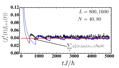
Figure 1: (color online) Time evolution of the correlation function of the local operator $O(x_{i})=f_{i}$ for $i=L/2$ and $L/2+1$, $\langle f^{{\dagger}}_{i}(t)f_{i+1}(t)\rangle$, for $L=800$ and $L=1600$, with $N=40$ and $N=80$ . The horizontal line corresponds to the time average for the largest system size ($L=1600$ and $N=80$). In the initial state $N=40$ ($N=80$) hardcore bosons that are confined by a harmonic potential of the form $V_{0}(x_{i}-x_{M})^{2}$, with $V_{0}=10^{-3}\>J/\sqrt{N}$ and $x_{M}=L/2$.

In order to demonstrate Eq. (42), we display in Fig. 1. the results of the numerical evaluation of the time evolution of $C_{ff}^{(2)}(x_{i},x_{i+1},t)$ ($i=L/2$) using Eq. (41) for $O(x_{i})=f_{i}$. We consider an initial state $\rho_{0}$ for which $V_{0}(k,k^{\prime})$ in Eq. (40) is a harmonic potential that confines $N$ hardcore bosons at the center of an open chain of $L$ sites. The potential $V_{0}(k,k^{\prime})$ is taken to scale as $V_{0}/\sqrt{N}$ ($V_{0}=10^{-3}\,J$ in Figs. 1,2, and 3) in order to obtain a well defined thermodynamic limit of the initial cloud of hardcore bosons Cassidy ; RigolMuramatsu . This potential is switched off at $t=0$ and the bosons are allowed to expand Rigol_gge . The vertical line in this figure corresponds to the time average (for $L=1600$, the average for $L=800$ is not shown but it is very close to it). The average is given by Eq. (43) evaluated at finite $L$. It can be seen from Fig. 1 that for both $L=800$ and $L=1600$, after a short transient, the correlation function exhibits roughly equilibrationa and its time fluctuations about the average become fairly small. In can be also seen that, as $L$ increases from $800$ to $1600$ (while keeping $N/L$ constant), the size of the time fluctuations decreases suggesting that for $L\to+\infty$ they will vanish. Therefore, in the thermodynamic limit the asymptotic correlations are given by the quasi-particle occupation $N_{0}(k)$. In the Appendix B, we further explore the equivalence between the thermodynamic limit of time-averaged correlations and their $t\to+\infty$ limit after taking the thermodynamic limit.

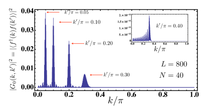
Figure 2: (color online) Modulus square of the eigenmode correlations, $|G_{0}(k,k^{\prime})|^{2}=|\langle f^{{\dagger}}(k)f(k^{\prime})\rangle|^{2}$ in the initial state of a XX chain at $T=0$, for a system in a box of size $L=800$ containing $N=40$ hardcore bosons, and $k^{\prime}/\pi=0.05,0.1,0.2,0.3$ and $0.4$ (inset). The initial state describes $N=40$ hardcore bosons that are confined by a harmonic potential with the same parameters as in Fig. 1. Note that the eigenmode correlations $|G_{0}(k,k^{\prime})|^{2}$ are strongly peaked at $k=k^{\prime}$. For $k>k_{0}$ with $k_{0}/\pi\simeq 0.35$ for $N=40$ (see inset) the correlations are no longer peaked at $k\simeq k^{\prime}$. However, they become substantially smaller than the typical peak values at $k^{\prime}<k_{0}$ ($k_{0}$ increases with $N$, cf. Fig. 4).

To understand the behavior displayed in Fig. 1 in physical terms, note that, in the thermodynamic limit, the sums over $k$ and $k^{\prime}$ in the expression for $C^{(2)}_{O}(x_{i},x_{j},t)$ become integrals and dephasing between different eigenmode contributions to Eq. (41) leads to the decay in time of the correlations except for the terms where $\epsilon(k)=\epsilon(k^{\prime})$. It is worth investigating how this dephasing takes place in more detail because, generally speaking, for non-translationally invariant states, $G_{0}(k,k^{\prime})$ is not generally speaking a smooth function of $k$ and $k^{\prime}$ (cf. figure 2 and 3). Thus, arguments based on the Riemann-Lebesgue lemma similar to those employed in sections II and III for translationally invariant states are not applicable. However, for non-translationally invariant states (i.e. $V_{0}(k,k^{\prime})\neq 0$), we numerically find that, as the thermodynamic limit is approached (cf. Fig. 3)

$$|G_{0}(k,k^{\prime})|^{2}\to N^{2}_{0}(k)\delta_{k,k^{\prime}}+\Delta R_{0}(k,k^{\prime}),$$ (43)

where $\Delta R_{0}(k,k^{\prime})$ decays rapidly for $|k-k^{\prime}|\gg L^{-1}$. Eq.(43) must be understood as the statement that typical correlations become strongly peaked at $k=k^{\prime}$ as $L\to+\infty$. Thus, setting $G_{0}(k,k^{\prime})\simeq N_{0}(k)\delta_{k,k^{\prime}}$ in Eq. (41) becomes an increasingly good approximation at large $t$ where decoherence acts most efficiently on the contributions to the double sum (41) of quasi-particle levels $k$ and $k^{\prime}$ that are close in energy and correlated (i.e. for which $G_{0}(k,k^{\prime})$ is not negligibly small).

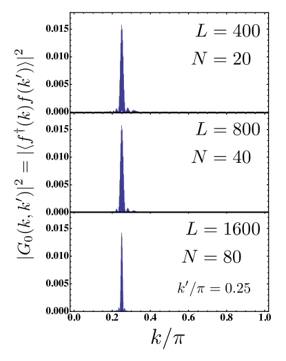
Figure 3: (color online) Finite-size scaling of the Modulus square of the eigenmode correlations, $|G_{0}(k,k^{\prime})|^{2}=|\langle f^{{\dagger}}(k)f(k^{\prime})\rangle|^{2}$ for the same initial state of a XX chain as described in the caption of Figs. 1 and 2 for systems of size $L=400,800,1600$ and $k^{\prime}/\pi=0.25$. Note that the peak becomes narrower as the system approaches the thermodynamic limit where $N$ and $L\to+\infty$ while $n_{0}=N/L=$ const.

The claim of Eq. (43) is illustrated in figures 2 and 3 for the same system used to generate Fig. 1. Fig. 2 displays $|G_{0}(k,k^{\prime})|^{2}$ as a function of $k$ for several values of $k^{\prime}$, for a system of $L=800$ sites and $N=\sum_{k}N_{0}(k)=40$ hardcore bosons at $T=0$. It can be seen that $|G_{0}(k,k^{\prime})|^{2}$ is strongly peaked at $k=k^{\prime}$ for $k^{\prime}<k_{0}$ ($k_{0}/\pi\simeq 0.35$ for $N=40$). However, for $k^{\prime}>k_{0}$ (see inset) the peak is no longer at $k=k^{\prime}$. In this case, however, the values of $|G_{0}(k,k^{\prime})|^{2}$ become very small compared to typical the peak values of $|G_{0}(k,k^{\prime})|^{2}$ for $k<k_{0}$. The cut-off $k_{0}$ is determined by the number of hardcore bosons in initial state $N\propto L$ (see discussion below and Fig. 4).

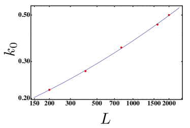
Figure 4: (color online) Log-log plot of the size dependence of the cut-off $k_{0}$ for $n_{0}=N/L=0.05$. The continuous curve is just a gide to the eye. Other parameters are the same used to generate figures 1, 2, and 3.

As the system size $L$ increases while keeping the lattice filling $n_{0}=N/L$ constant and scaling the initial trap strength as $V_{0}/\sqrt{N}$ RigolMuramatsu , the peak of $G_{0}(k,k^{\prime})$ at $k=k^{\prime}$ becomes substantially narrower (cf. Fig. 3). We also found a similar behavior of $G_{0}(k,k^{\prime})$ when the potential that initially acts upon the hardcore bosons was taken to be an extended superlattice unpub and an infinite square well box of size smaller than $L$ unpub2 . Although we cannot find a rigorous mathematical proof that Eq. (43) holds for any non-translationally invariant initial state of the form $\rho_{0}\sim e^{-H_{0}/T}$, with $H_{0}$ given by (40). we expect it to hold for any physically sensible scattering potential $V_{0}(k,k^{\prime})$. The following physical argument can be used to support this expectation. Recalling the relationship between the eigenmodes of $H$ and the eigenmodes of the initial Hamiltonian, $H_{0}$, the two sets of operators are related by the canonical transformation, $f(k)=\sum_{\alpha}\phi_{\alpha}(k)f(\alpha)$; $\phi_{\alpha}(k)$ are the eigenfunctions of $H_{0}$ in the basis of eigen orbitals of $H$, that is, $\phi_{\alpha}(k)=\langle k|\alpha\rangle$ where $H_{0}|\alpha\rangle=(\epsilon_{\alpha}-\mu)|\alpha\rangle$. Hence,

$$G_{0}(k,k^{\prime})=\sum_{\alpha=1}^{L}\phi^{*}_{\alpha}(k)\phi_{\alpha}(k^{\prime})F(\epsilon_{\alpha},T),$$ (44)

where $F(\epsilon_{\alpha},T)=\left[e^{(\epsilon_{\alpha}-\mu)/T}+1\right]^{-1}$ are the thermal occupations of the orbitals $\phi_{\alpha}(k)$ in the initial state and $\mu$ is the chemical potential. The latter allows us to fix the average number of quasi-particles in the initial state. Next, we notice that, as the thermodynamic limit is approached (i.e. $L\to+\infty$ while keeping the lattice filling $n_{0}=N/L$ constant), Eq. (44) becomes an infinite sum. Correlations are maximized for $k=k^{\prime}$ because the summands, $|\langle\alpha|k\rangle|^{2}$ are all positive and correspond to the probability that a quasi-particle initially found in the state $|\alpha\rangle$ ends up in the state $|k\rangle$ after the quench. On the other hand, for $|k-k^{\prime}|\gg L^{-1}$, the eigenmodes become largely uncorrelated because the sum in Eq. (44) involves a large number of complex amplitudes $\langle k|\alpha\rangle\langle\alpha|k^{\prime}\rangle=\phi^{*}_{\alpha}(k)\phi_{\alpha}(k^{\prime})$, describing the quantum interference between transitions where the quasi-particle ends in one of two orthogonal orbitals, either $|k\rangle$ or in $|k^{\prime}\rangle$. As $L\to+\infty$, the amplitudes interfere destructively and typically average to zero. Furthermore, at low temperatures, the sum  (44) contains a cut-off which is roughly given by the state $\alpha_{\max}$ for which $F(\epsilon_{\alpha_{\max}}-\mu)\ll 1$. Thus, for example, for $T=0$, $|\alpha_{\max}\rangle$ corresponds to the orbital with the $N$-th smallest eigenvalue $\epsilon_{\alpha}-\mu$. As $k=k^{\prime}$ increases, the number of nodes of the orbital $|k\rangle$ in the initially (harmonically) confined region increases, and the overlaps $\phi_{\alpha}(k)=\langle k|\alpha\rangle$ dramatically decrease in magnitude. This explains the existence of the cut-off $k_{0}$ seen in Fig. 2. Consistent with this effect, we numerically observe (see Fig. 4) that $k_{0}$ increases as the number of hardcore bosons $N$ increases, which makes $\alpha_{\max}$ bigger. At higher temperatures, the increase in entropy implies that quasi-particles are spread even more over the set of initial orbitals $|\alpha\rangle$, and the quantum interference effects will be weakened thus decreasing the correlations $|G_{0}(k,k^{\prime}\neq k)|^{2}$ even further.

To end this section, we shall use the above results to sketch the proof that the momentum distribution function of the hardcore bosons, $S(q,t)$, for $t\to+\infty$ is also nonergodic. We first recall that

$$S(q,t) =\frac{1}{L}\sum_{ij}e^{iq(x_{i}-x_{j})}\>\langle\sigma^{-}_{i}(t)\sigma^{+}_{j}(t)\rangle$$ (45)

$$=\frac{2}{L}\sum_{ij}e^{iq(x_{i}-x_{j})}\>C^{(2)}_{xx}(x_{i},x_{j},t),$$ (46)

where $C^{(2)}_{xx}(x_{i},x_{j},t)=\langle\sigma^{x}_{i}(t)\sigma^{x}_{j}(t)\rangle$. The latter correlation function involves the operator $\sigma^{x}$ that is nonlocal in the eigenmodes $f(k),f^{{\dagger}}(k)$. However, using Wick’s theorem, it can be written in terms of products of two-point correlation functions of the local operators $A_{i}=f^{{\dagger}}_{i}+f_{i}$ and $B_{i}=f^{{\dagger}}_{i}-f_{i}$. The $t\to+\infty$ limit of the product exists provided the $t\to+\infty$ limit of the two-point correlation functions involved in the product also exists (see the extended discussion in Appendix B). Moreover, as $t\to+\infty$

$$\langle A_{i}(t)A_{j}(t)\rangle \to\delta_{ij},$$ (47)

$$\langle B_{i}(t)B_{j}(t)\rangle \to-\delta_{ij}.$$ (48)

Hence, the $t\to+\infty$ limit of $C^{(2)}_{xx}(x_{i},x_{j},t)$ reduces to a Toeplitz determinant involving $\lim_{t\to+\infty}\langle A_{i}(t)B_{j}(t)\rangle=D^{(2)}_{AB}(x_{i},x_{j})$ only (cf. Appendix C), where

$$D^{(2)}_{AB}(x_{i},x_{j})=-\delta_{ij}+2\sum_{k}\varphi^{*}_{k}(x_{i})\varphi_{k}(x_{j})N_{0}(k),$$ (49)

with $\varphi_{k}(x_{i})=\sqrt{2/(L+1)}\sin kx_{i}$. This result implies that $D^{(2)}(x_{i},x_{j})$ is nonergodic. Hence, $C^{(2)}_{xx}(x_{i},x_{j},t\to+\infty)$ and $S(q,t\to+\infty)$ are also nonergodic.

V Discussion, Summary, and Outlook

We have shown that, in exactly solvable models, the correlation functions of both local and non-local operators, at asymptotically long times, are functions of the quasi-particle occupations in the initial state, for a broad class of initial states. This means that correlation functions in these systems retain much more memory of the initial conditions than in systems relaxation to thermal equilibrium, which is described by a standard Gibbs ensemble. This lack of relaxation is similar to the observations of McCoy McCoyII and Mazur Mazur for the magnetization in the XY model. It implies equilibration Reimann but lack of ergodicity Mazur , as the existence of non trivial integrals of motion strongly constraints the system dynamics and prevents it from reaching thermal equilibrium and exploring all possible states having the same average energy and particle number (grand canonical Gibbs ensemble).

By using the reduced density matrices for this class of initial states, we can show that nonergodicity implies that the asymptotic correlation functions can be effectively described by an ensemble that assigns a mode-dependent temperature to each eigenmode. This is precisely the physical content of the generalized Gibbs ensemble (GGE) Rigol_gge . We have illustrated our method by analyzing the the quantum Ising and the XX spin chain models, both of which exhibit fermionic quasi-particles. In Sec. III, the Luttinger model, which exhibits bosonic quasi-particles, was analyzed by the same method.

For initial states lacking the lattice translational symmetry, we have shown the connection between nonergodicity and the fact that eigenmode correlations in the initial state become dominated by diagonal correlations (i.e. quasi-particle occupations) as the thermodynamic limit is approached. By direct numerical calculation and physical reasoning, we have argued that this property should hold true for quantum quenches in which a physically sensible potential (e.g. a trap) that scatters the quasi-particles is suddenly removed at $t=0$. However, at present we are unable to provide a mathematically rigorous proof of this fact (cf. Eq. 43), although in all cases that we have examined so far, it appears to hold true.

Furthermore, using method reported here, we have been able to analytically shed light, for a much broader class of exactly solvable models and initial states than considered so far Cazalilla ; Calabrese_Ising , on the conditions under which the generalized Gibbs ensemble is expected to apply. Thus, our results extend the validity of the GGE conjecture to a much broader class of quantum quenches. Our method also explains the special role played by the quasi-particle occupation operators as the set of integrals of motion required to construct the GGE. The nonergodic behavior of the correlation functions found here is entirely explained by the dependence on the expectation value of such integrals of motion alone.

In future studies unpub ; unpub2 , it will interesting to understand how these results relate to the generalized eigenstate thermalization hypothesis discussed in Ref. Cassidy . We will also apply our methods to understand the conditions under which the asymptotic state can become arbitrarily close to a thermal state unpub . The latter study unveils further interesting connections between the GGE and quantum Information theory unpub .

Appendix A Eigenmodes of the quantum Ising and XX chains

The Hamiltonian of the XX and Quantum Ising chains introduced in the main text can be brought to diagonal form by means of the Jordan-Wigner transformation:

$$\sigma^{z}_{i} =1-2f^{{\dagger}}_{i}f_{i},\quad\sigma^{+}_{i}=\prod_{j<i}(1-2f^{{\dagger}}_{j}f_{j})f_{i},$$ (50)

$$\sigma^{x} =\frac{1}{2}(\sigma^{+}_{i}+\sigma^{-}_{i}),\quad\sigma^{-}_{i}=\left(\sigma^{+}_{i}\right)^{{\dagger}}$$ (51)

with $\{f_{i},f^{{\dagger}}_{j}\}=\delta_{ij}$, anti-commuting otherwise.

For the Quantum Ising chain, assuming periodic boundary conditions, that is,

$$f_{j}=\left(\frac{1}{L}\right)^{1/2}\sum_{k}\,e^{ikx_{j}}f(k),$$ (52)

with $x_{j}=j$ and

$$f(k)=\cos(\theta_{g}(k)/2)\gamma(k)+i\sin(\theta_{g}(k)/2)\gamma^{{\dagger}}(-k),$$ (53)

where $\tan\theta_{g}(k)=\sin k/(\cos k-g)$. These two transformations render the Hamiltonian of the Quantum Ising chain, Eq. 2, diagonal:

$$H=\sum_{k}\epsilon_{g}(k)\left[\gamma^{{\dagger}}(k)\gamma(k)-\frac{1}{2}\right],$$ (54)

where $\epsilon_{g}(k)=2J\sqrt{1+g^{2}-2g^{2}\cos k}$.

For the XX chain we shall assume an open ended chain where

$$f_{j}=\left(\frac{2}{L+1}\right)^{1/2}\sum_{k}\sin kx_{j}\>f(k),$$ (55)

with $k=\frac{\pi m}{L+1}$, $j,m=1,\ldots,L$, yields:

$$H=\sum_{k}\epsilon(k)f^{{\dagger}}(k)f(k),$$ (56)

where $\epsilon(k)=-J\cos k-h$.

Appendix B Time averages and Wick’s theorem

As mentioned in the main text, the calculation of asymptotic correlation functions of non-local operators like $\sigma^{x}_{j}$ in the quantum Ising and XX chain models depends on the applicability of Wick’s theorem in the $t\to+\infty$ limit to multi-point correlation functions. Thus, we shall first tackle this problem by time-averaging the correlation functions of finite systems prior to taking the thermodynamic limit. Let

$$C^{(2)}_{O}(x_{i},x_{j},t)=\langle O(x,t)O(0,t)\rangle,$$ (57)

for local operator like $O(x)=\sum_{k}\varphi_{k}(x)f_{k}$. Its time average is defined as:

$$\overline{C^{(2)}_{O}(x_{i},x_{j},t)}=\lim_{T\to+\infty}\frac{1}{T}\int^{T}_{0}dt\,C^{(2)}_{O}(x_{i},x_{j},t).$$ (58)

A priori, the time average of $C^{(2)}_{O}(x_{i},x_{j},t)$ followed by the thermodynamic limit yields

$$D^{(2)}_{O}(x_{i},x_{j}) =\sum_{k}\varphi^{*}_{k}(x_{i})\varphi_{k}(x_{j})N_{0}(k),$$

$$=\lim_{t\to+\infty}C^{(2)}_{O}(x_{i},x_{j},t),$$ (59)

where the last limit is taken after the thermodynamic limit. However, taking the thermodynamic limit after time averaging is a subtle procedure. For instance, for the four-point correlation,

$$C^{(4)}_{O}(x_{i},x_{j},x_{m},x_{n},t)=\langle O^{{\dagger}}(x_{i},t)O^{{\dagger}}(x_{j},t)\\ \times O(x_{m},t)O(x_{n},t)\rangle,$$ (60)

it yields:

$$\overline{C^{(4)}_{O}(x_{i},x_{j},x_{m},x_{n},t)}=\sum_{k,k^{\prime}}A_{k,k^{\prime}}(x_{i},x_{j},x_{m},x_{n})\\ \times\left[N_{0}(k)N_{0}(k^{\prime})-|G_{0}(k,k^{\prime})|^{2}\right],$$ (61)

where

$$A_{k,k^{\prime}}(x_{i},x_{j},x_{m},x_{n})=\varphi^{*}_{k}(x_{i})\varphi_{k}(x_{n})\varphi^{*}_{k^{\prime}}(x_{j})\varphi_{k^{\prime}}(x_{m})\\ -\varphi^{*}_{k}(x_{i})\varphi_{k}(x_{m})\varphi^{*}_{k^{\prime}}(x_{j})\varphi_{k^{\prime}}(x_{n}).$$ (62)

Since we have assumed that the square of the functions $\varphi_{k}(x_{i})$ is normalized to system size, i.e. $|\varphi_{k}(x_{i})|\sim O(L^{-1/2})$, it follows that $A_{k,k^{\prime}}(x_{i},x_{j},x_{m},x_{n})\sim O(L^{-2})$, which is required to obtain a finite result in the $L\to+\infty$ limit given the presence of the double sum over $k$ and $k^{\prime}$.

However, we note that

$$\overline{C^{(4)}_{O}(x_{i},x_{j},x_{m},x_{n},t)}\neq\overline{C^{(2)}_{O}(x_{i},x_{n},t)}\,\,\overline{C^{(2)}_{O}(x_{j},x_{m},t)}\\ -\overline{C^{(2)}_{O}(x_{i},x_{m},t)}\,\,\overline{C^{(2)}_{O}(x_{j},x_{n},t)}.$$ (63)

and thus, if we also identify $D^{(4)}(x_{i},x_{j},x_{m},x_{n})=\lim_{t\to+\infty}C^{(4)}_{O}(x_{i},x_{j},x_{m},x_{n},t)$ with its time average, Wick’s theorem appears to be violated for $t\to+\infty$ in the thermodynamic limit as $D^{(4)}(x_{i},x_{j},x_{m},x_{n})$ will a priori depend on all quantum correlations between the eigenmodes described by $G_{0}(k,k^{\prime})$ (cf. Eq. 61). However, $D^{(2)}(x_{i},x_{j})$, which we identified with $\overline{C^{(2)}(x_{i},x_{j},t})$, only depends on $N_{0}(k)=G_{0}(k,k)$. This has implications for the calculation of correlation functions of non-local operators in the $t\to+\infty$ limit. Nevertheless, as it was discussed in the main text, the eigenmode correlations,

$$|G_{0}(k,k^{\prime})|^{2}\to\left[N_{0}(k)\right]^{2}\delta_{k,k^{\prime}}+\Delta R_{0}(k,k^{\prime}),$$ (64)

as the thermodynamic limit is approached. Therefore, the term involving these correlations in Eq. (61), becomes approximately equal (after neglecting $\Delta R_{0}(k,k^{\prime})$ to

$$-\sum_{k}A_{k,k}(x_{i},x_{j},x_{m},x_{n})N^{2}_{0}(k),$$ (65)

which is manifestly of $O(L^{-1})$ as $L\to+\infty$. On the other hand, the term

$$\sum_{k,k^{\prime}}A_{k,k^{\prime}}(x_{i},x_{j},x_{m},x_{n})N_{0}(k)N_{0}(k^{\prime})$$ (66)

is of $O(L^{0})$ as $L\to+\infty$. However, Eq. (66) equals the anti-symmetrized product of the time averaged two-point correlation functions, $\overline{C^{(2)}(x_{i},x_{j})}$. Thus, the fact that the contribution of non-diagonal correlations becomes negligible in the thermodynamic limit justifies the procedure to taking the time-average followed by the thermodynamic limit.

We can try to extend the above result to higher order (i.e. $3$-point, etc.) correlation correlation functions. However, it is more convenient to take a shortcut. As discussed in the previous paragraph, we can identify the time average of two-point correlation functions of local operators like $O(x)$ with the $t\to+\infty$ limit of the same correlation function in the thermodynamic limit. These two point correlation function are the building blocks for computing with multi-point correlation functions or correlation functions of non-local operators like $\sigma^{x}$ as we can apply Wick’s theorem first and then let $t\to+\infty$ using

$$\lim_{t\to+\infty}c_{1}(t)c_{2}(t)\cdots c_{M}(t)=\prod_{i=1}^{M}c_{i}(+\infty)$$ (67)

where $c_{i}(+\infty)=\lim_{t\to+\infty}c_{i}(t)$ since the $t\to+\infty$ limit of two-point every correlation function ($c_{i}(t)$ in the expression above) exist and it is given by the its time average followed by the thermodynamic limit.

Appendix C Non-local correlations in the quantum Ising and XX chain

For the XX chain, the momentum distribution of the hardcore bosons can be obtained from the expression:

$$S(q,t)=\frac{1}{2L}\sum_{ij}e^{iq(x_{i}-x_{j})}\>C^{(2)}_{xx}(x_{i},x_{j},t),$$ (68)

for $t\to+\infty$ can be computed first using Wick’s theorem and letting $t\to+\infty$ in the resulting expression. To this end, it is convenient to write $\sigma^{x}_{i}(t)=A_{i}(t)\prod_{j<i}A_{j}(t)B_{j}(t)$, being

$$A_{i}(t) =f^{{\dagger}}_{i}(t)+f_{i}(t)=\left(\frac{2}{L+1}\right)^{1/2}\sum_{k}\sin kx_{i}\>\big{[}e^{i\epsilon(k)t/\hbar}$$

$$\times f^{{\dagger}}(k)+e^{-i\epsilon(k)t/\hbar}\>f(k)\big{]},$$ (69)

$$B_{i}(t) =f^{{\dagger}}_{i}(t)-f_{i}(t)=\left(\frac{2}{L+1}\right)^{1/2}\sum_{k}\sin kx_{i}\>\big{[}e^{i\epsilon(k)t/\hbar}$$

$$\times f^{{\dagger}}(k)-e^{-i\epsilon(k)t/\hbar}\>f(k)\big{]}.$$ (70)

where the mode expansions are given for the XX chain (cf. e.g. Ref. Sengupta04 for the corresponding expressions for the quantum Ising chain). Hence,

$$C^{(2)}_{xx}(x_{i},x_{j},t)=\langle B_{i}(t)\left[\prod_{i<l<j}A_{l}(t)B_{l}(t)\right]A_{j}(t)\rangle,$$ (71)

where we have assumed that $x_{i}<x_{j}$ without loss of generality. To evaluate the expression above we use Wick’s theorem and take the limit $t\to+\infty$ of the resulting expression only after taking the thermodynamic limit. Moreover, since

$$\langle A_{i}(t)A_{j}(t)\rangle \to\delta_{ij},$$ (72)

$$\langle B_{i}(t)B_{j}(t)\rangle \to-\delta_{ij},$$ (73)

the correlation function

$$D_{xx}(x_{i},x_{j})=\lim_{t\to+\infty}C_{xx}(x_{i},x_{j},t)$$ (74)

can be written as a Toeplitz determinant McCoyI :

$$D_{xx}(x_{i},x_{j}) = \left|\begin{array}[]{cccc}a_{0}&a_{1}&\cdots&a_{-n+1}\\ a_{1}&a_{0}&\cdots&a_{-n+2}\\ \vdots&\vdots&\ddots&\vdots\\ a_{n-1}&a_{n-2}&\cdots&a_{0}\end{array}\right|,$$ (79)

where $a_{i-j+1}=-D^{(2)}_{AB}(x_{i},x_{j})$, and

$$D^{(2)}_{AB}(x_{i},x_{j})=\lim_{t\to+\infty}\langle A_{i}(t)B_{j}(t)\rangle\\ =-\delta_{ij}+2\sum_{k}\varphi^{*}_{k}(x_{i})\varphi_{k}(x_{j})N_{0}(k),$$ (80)

where $\varphi_{k}(x_{i})=\sqrt{2/(L+1)}\sin kx_{i}$ and the thermodynamic limit $L\to+\infty$ at finite lattice filling, $n_{0}=N/L$, is implicitly understood. Note that, in this limit, the actual boundary conditions (open or otherwise) are irrelevant.

References

- (1) T. Kinoshita, T. Wenger, and D. S. Weiss, Nature (London) 440, 900 (2006).
- (2) S. Hofferberth et al. Nature (London) 449, 324 (2007).
- (3) M. Greiner et al., Nature (London) 419, 51 (2002). S. Trotsky et al. arxiv: 1101.2658 (2011).
- (4) M. Rigol, V. Dunjko, V. Yurovsky, and M. Olshanii, Phys. Rev. Lett. 98, 050405 (2007); M. Rigol, A. Muramatsu, and M. Olshanii, Phys. Rev. A 74, 053616 (2006)
- (5) M. A. Cazalilla, Phys. Rev. Lett 97 156403 (2006); A. Iucci and M. A. Cazalilla, Phys. Rev. A 80, 063619 (2009);
- (6) E. Altman and A. Auerbach, Phys. Rev. Lett. 89, 250404 (2002); P. Calabrese and J. Cardy, ibid 96, 136801 (2006); S. R. Manmana, S. Wessel, R. M. Noack, and A. Muramatsu, ibid 98 210405 (2007); M. Eckstein and M. Kollar, ibid 100, 120404 (2008); P. Reimann, ibid 101, 190403 (2008); P. Barmettler, M. Punk, V. Gritsev, E. Demler, and E. Altman, ibid 102, 130603 (2009); M. Moeckel and S. Kehrein ibid 100 175702 (2008); D. Sen, K. Sengupta, and S. Mondal, ibid 101, 016806 (2008); D. Pataè et al., ibid 245701 (2009); D. M. Gangardt and M. Pustilnik, Phys. Rev. A 77, 041604(R) (2008); A. Faribault, P. Calabrese, and J.-S. Caux, J. Stat. Mech.: Theory Exp. (2009) P03018; C. De Grandi, V. Gritsev, A. Polkovnikov Phys. Rev. B 81, 012303 (2010); ibid 81, 224301 (2010); L. F. Santos, M. Rigol, and A. Polkovnikov, arXiv:1103.0557 (2011).
- (7) M. A. Cazalilla and M. Rigol, New J. of Phys. 12 055006 (2010).
- (8) See A. Polkovnikov, K. Sengupta, A. Silva, M. Vengalattore, Rev. Mod. Phys. 83, 863 (2011).
- (9) V. Gritsev and A. Polkovnikov in Understanding Quantum Phase Transitions, ed. by L. D. Carr (Taylor & Francis, Boca Raton, 2010)
- (10) E. T. Jaynes, Phys. Rev. 106, 620 (1957); ibid 108, 171 (1957).
- (11) D. Rossini, A. Silva, G. Mussardo, and G. Santoro, Phys. Rev. Lett. 102, 127204 (2009); T. Caneva, E. Canovi, D. Rossini, G. E. Santoro, and A. Silva, : J. Stat. Mech. P07015 (2011).
- (12) P. Calabrese, F. H L. Essler, and M. Fagotti, Phys. Rev. Lett. 106, 227203 (2011).
- (13) A. Iucci and M. A. Cazalilla, New Journal of Physics 12, 055019 (2010).
- (14) D. Fioretto and G. Mussardo, New J. of Phys. 12, 055015 (2010).
- (15) A. Cassidy, C. W. Clark, and M. Rigol, Phys. Rev. Lett. 106, 140405 (2011).
- (16) M. Rigol, V. Dunjko, and M. Olshanii, Nature (London) 452, 854 (2008).
- (17) M. Srednicki, Phys. Rev. E 50, 888 (1994); J. Deutsch, Phys. Rev. A 43, 2046 (1991).
- (18) E. Baruch and B. M. McCoy, Phys. Rev. A 2, 1075 (1970); see also J.H.H. Perk, H.W. Capel, and Th.J. Siskens, Physica A 89, 304 (1977).
- (19) P. Mazur, Physica 43, 533 (1969).
- (20) K. Sengupta, S. Powell, and S. Sachdev, Phys. Rev. A 69, 053616 (2004).
- (21) P. Reimann, Phys. Rev. Lett. 101, 190403 (2008).
- (22) See e.g. N. N. Bogolubov and N. N. Bogolubov Jr., Introduction to Quantum Stastistical Mechanics, 2nd edition (Singapore, 2010), pag. 282, for a proof.
- (23) S.-A. Cheong and C. L. Henley, Phys. Rev. B 69, 075111 (2004); I. Peschel, J. Phys. A 36, L205 (2003); T. Barthel, M.-C. Chung, and U. Schollwöck Phys. Rev. A 74, 022329 (2006)
- (24) M.C. Chung and I. Peschel , Phys. Rev. B 64, 064412 (2001).
- (25) M. Rigol and A. Muramatsu, Phys. Rev. A 70, 031603(R) (2004).
- (26) M. C. Chung, M. A. Cazalilla, and A. Iucci, in preparation.
- (27) A. Iucci, M. C. Chung, and M. A. Cazalilla, in preparation.
- (28) E. Lieb, T. Schultz, and D. Mattis, Ann. Phys. (N. Y.) 16, 206 (1961); E. Baruch and B. M. McCoy, Phys. Rev. A 3, 786 (1971).
- (29) D. C. Mattis and E. H. Lieb, J. Math. Phys. 6, 304 (1965); A. Luther and I. Peschel, Phys. Rev. B 9, 2911 (1974); T. Giamarchi, Quantum Physics in One Dimension, (Oxford University Press Oxford, 2004).