Thermoelectric transport with electron-phonon coupling and electron-electron interaction in molecular junctions

Abstract

Within the framework of nonequilibrium Green’s functions, we investigate the thermoelectric transport in a single molecular junction with electron-phonon and electron-electron interactions. By transforming into a displaced phonon basis, we are able to deal with these interactions nonperturbatively. Then, by invoking the weak tunneling limit, we are able to calculate the thermoelectricity. Results show that at low temperatures, resonances of the thermoelectric figure of merit, $ZT$, occur around the sides of resonances of electronic conductance but drop dramatically to zero at exactly these resonant points. We find $ZT$ can be enhanced by increasing electron-phonon coupling and Coulomb repulsion, and an optimal enhancement is obtained when these two interactions are competing. Our results indicate a great potential for single molecular junctions as good thermoelectric devices over a wide range of temperatures.

I Introduction

Recently, the potential afforded by nanoscale engineering Snyder08 has revitalized interest in developing novel thermoelectric materials for the generation and harvesting of energy. It is well accepted that nanoscale materials engineering in principle creates unlimited opportunities for the creation of more efficient energy-conversion devices Dresselhaus07 and thus expands the potential of using thermoelectricity for meeting the challenge of being a sustainable energy source. Majumdar04 However, questions remain about the best ways for manipulating the microscopic properties of the material so that enhanced performance occurs. Majumdar04 ; Mahan96

The thermoelectric performance is typically characterized by the figure of merit, $ZT$, Mahan96 ; Dubi11 which is defined as $ZT={G_{e}S^{2}T}/{\kappa}$, where $G_{e}$ is the electronic conductance, $S$ is the thermopower, $T$ is the temperature, and $\kappa$ is the thermal conductance. Increasing the value of $ZT$ increases the efficiency of heat-electricity conversion. The dependence of the figure of merit on both charge and energy transport shows that thermoelectric efficiency is strongly affected by the underlying electronic and vibrational properties of a material. These dependencies are especially transparent in molecular junctions, Reddy07 as charge accumulation on the junction causes Coulomb interactions (e-e) to perturb the electronic structure ee02 and the electron-phonon (e-ph) coupling to perturb the vibrational modes and the conformation of the junction. Galperin07

The energy scale of e-e interaction is usually much larger than that of e-ph interaction. However, at the atomic and molecular levels, the electrodes can screen the Coulomb repulsion, reducing it to the same order of magnitude as the e-ph interaction. The interactions now compete. Thus, it is of fundamental and practical importance to explore the effects of this competition to gain insights into the optimization of thermoelectric transport for better energy-conversion devices.

In this work, we investigate the thermoelectric transport in a single molecular junction with e-e interaction and e-ph coupling of arbitrary strengths in the framework of the nonequilibrium Green’s function (NEGF) method. Haugbook Although there are considerable efforts toward understanding the effects of the e-e Murphy08 ; Costi10 ; Liu10 ; Wysokinski10 or e-ph Wohlman10 ; Zianni10 interactions, what happens to the thermoelectric transport when e-ph coupling competes with e-e interaction in a full range of strength is still an open question. In contrast to previous work in the literature, Koch04 ; Leijnse10 we treat the e-e and e-ph interactions within the molecular junction nonperturbatively, by a transform of the phonon basis with effective displacements. This treatment moves our use of the NEGF framework beyond the weak e-ph coupling perturbative analysis, eph09 ; Wohlman10 ; Paulsson05 the strong e-ph coupling limit of canonical transformation (the Lang-Firsov approach), Zhu03Chen05 ; Mahanbook ; Kuo10 and the mean-field approximation in the strong Coulomb repulsion regime. Liu10 ; Kuo10

II Method and Approximation

We start with the standard Anderson-Holstein Hamiltonian: AHM1 ; AHM2 $H=H_{\text{mol}}+H_{\text{T}}+H_{\text{leads}}$. $H_{\text{mol}}$ describes the molecular junction of one orbital level, with Coulomb repulsion between electrons of opposite spin orientations and additional coupling to the vibration of itself, which is conventionally assumed to be: Haugbook ; Koch04 ; Leijnse10 ; Kuo10 ; Mahanbook ; AHM1 ; AHM2

$$H_{\text{mol}}=\omega_{0}\hat{a}^{{\dagger}}\hat{a}+\sum_{\sigma}\varepsilon_{\sigma}\hat{d}^{{\dagger}}_{\sigma}\hat{d}_{\sigma}\\ +\sum_{\sigma}\lambda_{\sigma}\hat{d}^{{\dagger}}_{\sigma}\hat{d}_{\sigma}(\hat{a}^{{\dagger}}+\hat{a})+U\hat{d}^{{\dagger}}_{\uparrow}\hat{d}_{\uparrow}\hat{d}^{{\dagger}}_{\downarrow}\hat{d}_{\downarrow}.$$

In the first term on the right-hand side, $\hat{a}^{{\dagger}}$ and $\hat{a}$ create and annihilate a phonon with energy $\omega_{0}$ while in the second term $\hat{d}^{{\dagger}}_{\sigma}$ and $\hat{d}_{\sigma}$ create and annihilate an electron of spin $\sigma$ at the molecular level with energies $\varepsilon_{\uparrow}=\varepsilon_{0}+\Delta\varepsilon/2$ or $\varepsilon_{\downarrow}=\varepsilon_{0}-\Delta\varepsilon/2$. The third and fourth terms describe the e-ph and e-e interactions with strengths $\lambda_{\sigma}$ and $U$. The expression

$$H_{\text{leads}}=\sum_{k,\sigma,\nu=\text{L,R}}\epsilon^{\nu}_{k\sigma}N^{\nu}_{k\sigma}.$$

describes the left and right electrode leads with $N^{\nu}_{k\sigma}=\hat{c}^{{\dagger}}_{k\sigma\nu}\hat{c}_{k\sigma\nu}$ the number operator for electrons of reservoir $\nu$ with wave number $k$ and spin $\sigma$. The expressoin

$$H_{\text{T}}=\sum_{k,\sigma,\nu=\text{L,R}}t^{\nu}_{k\sigma}(\hat{d}^{{\dagger}}_{\sigma}\hat{c}_{k\sigma\nu}+\hat{d}_{\sigma}\hat{c}^{{\dagger}}_{k\sigma\nu})$$

describes the tunneling Hamiltonian of the electron hopping between the molecule and the electrode leads. Here, due to the large mismatch of vibrational spectra between the molecule and metallic electrodes, the phonon transport is not considered.

Computing the transport for this model within the NEGF formalism requires the knowledge of various Green’s functions for the different parts of $H$. We start by analytically solving the eigenproblem for the molecular part of the junction. The Hilbert space of the molecular part is spanned by the basis {$|\vartheta,n\rangle$}, where $|\vartheta\rangle$ are the four possible electron states $|\o\rangle$, $|\sigma\rangle$, $|\bar{\sigma}\rangle$, $|\sigma\bar{\sigma}\rangle$ and $|n\rangle$ denotes phonon states with $n=0,1,\ldots,\infty$. To nonperturbatively treat the e-ph and e-e interactions with arbitrary strengths, we first block diagonalize the Hamiltonian with respect to electron states:

$$\langle\o|H_{\mathrm{mol}}|\o\rangle = \omega_{0}\hat{a}^{{\dagger}}\hat{a},$$

$$\langle\sigma|H_{\mathrm{mol}}|\sigma\rangle = \omega_{0}\hat{a}^{{\dagger}}\hat{a}+\varepsilon_{\sigma}+\lambda_{\sigma}(\hat{a}^{{\dagger}}+\hat{a}),$$

$$\langle\sigma\bar{\sigma}|H_{\mathrm{mol}}|\sigma\bar{\sigma}\rangle = \omega_{0}\hat{a}^{{\dagger}}\hat{a}+\sum_{\sigma}\varepsilon_{\sigma}+\sum_{\sigma}\lambda_{\sigma}(\hat{a}^{{\dagger}}+\hat{a})+U.$$

It is easy to further diagonalize $\langle\o|H_{\mathrm{mol}}|\o\rangle$ with conventional Fock phonon states: $|n\rangle_{\o}=|n\rangle=[(\hat{a}^{{\dagger}})^{n}/\sqrt{n!}]|0\rangle$. However, in order to diagonalize the other two matrix elements, we need introduce a new phonon basis, Chen08 ; Chen11 with displacements shifted by different electron states through the e-ph coupling:

$$|n\rangle_{\vartheta}=[{(\hat{A}^{{\dagger}}_{\vartheta})^{n}}/{\sqrt{n!}}]\exp{(-g_{\vartheta}^{2}/2-g_{\vartheta}\hat{a}^{{\dagger}})}|0\rangle,$$ (1)

where $\hat{A}^{{\dagger}}_{\vartheta}=\hat{a}^{{\dagger}}+g_{\vartheta}$ denotes the new creator that creates a phonon displaced from the original position by a value $g_{\vartheta}$ depending on the electronic state, that is, $g_{\o}=0$, $g_{\sigma}=\lambda_{\sigma}/\omega_{0}$, and $g_{\sigma\bar{\sigma}}=g_{\sigma}+g_{\bar{\sigma}}$. Clearly, when electrons are absent on the molecular quantum dot, $g_{\o}=0$ and the displaced phonon basis reduces to the normal Fock state of the phonons. We then can write

$$\langle\sigma|H_{\mathrm{mol}}|\sigma\rangle = \omega_{0}\hat{A}_{\sigma}^{{\dagger}}\hat{A}_{\sigma}+\varepsilon_{\sigma}-\omega_{0}g^{2}_{\sigma},$$

$$\langle\sigma\bar{\sigma}|H_{\mathrm{mol}}|\sigma\bar{\sigma}\rangle = \omega_{0}\hat{A}_{\sigma\bar{\sigma}}^{{\dagger}}\hat{A}_{\sigma\bar{\sigma}}+\varepsilon_{\sigma}+\varepsilon_{\bar{\sigma}}-\omega_{0}g^{2}_{\sigma\bar{\sigma}}+U.$$

Therefore, with the help of the new phonon basis, the solution to the eigenvalue problem is

$$H_{\mathrm{mol}}|\o,n\rangle_{\o} = n\omega_{0}|\o,n\rangle_{\o},$$ (2)

$$H_{\mathrm{mol}}|\sigma,n\rangle_{\sigma} = (n\omega_{0}+\tilde{\varepsilon}_{\sigma})|\sigma,n\rangle_{\sigma},$$ (3)

$$H_{\mathrm{mol}}|\sigma\bar{\sigma},n\rangle_{\sigma\bar{\sigma}} = (n\omega_{0}+\tilde{\varepsilon}_{\sigma\bar{\sigma}}+U)|\sigma\bar{\sigma},n\rangle_{\sigma\bar{\sigma}},$$ (4)

where

$$\tilde{\varepsilon}_{\sigma} =\varepsilon_{\sigma}-\omega_{0}g^{2}_{\sigma}$$

$$\tilde{\varepsilon}_{\sigma\bar{\sigma}} =\varepsilon_{\sigma}+\varepsilon_{\bar{\sigma}}-\omega_{0}g^{2}_{\sigma\bar{\sigma}}=\tilde{\varepsilon}_{\sigma}+\tilde{\varepsilon}_{\bar{\sigma}}-2\omega_{0}g_{\sigma}g_{\bar{\sigma}}.$$

The negative term $-2\omega_{0}g_{\sigma}g_{\bar{\sigma}}$ evidences the attractive interaction between different electron states induced by the e-ph coupling.

With $H_{\text{mol}}$ diagonalized, we can now analytically calculate the advanced and retarded Green’s functions of the molecule, which are found to be (see Appendix A for details)

$$G_{\sigma}^{r(a)}(\omega)=\frac{1}{Z}\sum^{\infty}_{n,m=0}\left[\frac{e^{-\beta m\omega_{0}}+e^{-\beta(n\omega_{0}+\tilde{\varepsilon}_{\sigma})}}{\omega-\Delta_{mn}^{(1)}\pm i0^{+}}+\right.\\ \left.\frac{e^{-\beta(m\omega_{0}+\tilde{\varepsilon}_{\bar{\sigma}})}+e^{-\beta(n\omega_{0}+\tilde{\varepsilon}_{\sigma\bar{\sigma}}+U)}}{\omega-\Delta_{mn}^{(2)}\pm i0^{+}}\right]D^{2}_{nm}(g_{\sigma}),$$ (5)

where

$$\Delta_{nm}^{(1)} =(n-m)\omega_{0}+\tilde{\varepsilon}_{\sigma},$$

$$\Delta_{nm}^{(2)} =(n-m)\omega_{0}+(\tilde{\varepsilon}_{\sigma}-2\omega_{0}g_{\sigma}g_{\bar{\sigma}}+U),$$

$$D_{nm}(g_{\sigma}) =(-1)^{m}{{}_{\o}}\langle m|n\rangle_{\sigma}=(-1)^{m}{}_{\bar{\sigma}}\langle m|n\rangle_{\sigma{\bar{\sigma}}}$$

$$=e^{-g_{\sigma}^{2}/2}\sum^{\mathrm{min}\{n,m\}}_{k=0}\frac{(-1)^{k}\sqrt{n!m!}g_{\sigma}^{n+m-2k}}{(n-k)!(m-k)!k!},$$

$$Z =(1+N_{\mathrm{ph}})(1+e^{-\beta\tilde{\varepsilon}_{\sigma}}+e^{-\beta\tilde{\varepsilon}_{\bar{\sigma}}}+e^{-\beta(\tilde{\varepsilon}_{\sigma\bar{\sigma}}+U)}).$$

Here $N_{\mathrm{ph}}=1/(e^{\beta\omega_{0}}-1)$ denotes the Bose distribution of the phonon population with inverse temperature $\beta\equiv k_{B}T$. Note, in the zero-temperature limit, Eq. (5) is consistent with the “atomic limit” Green’s functions in Refs. AHM2, ; Martin08, through using canonical transformation. The advantage of our method is that at finite temperatures our results still give Green’s functions analytically and explicitly, while for the atomic limit with the Lang-Firsov canonical transformation, the expressions of Green’s functions contain the electronic level occupation, the value of which must be found through a self-consistency iteration.

With the molecular part treated nonperturbatively, we now follow standard paths to build the Green’s functions of the molecule-lead-electrode system. By using the Dyson equation and the Keldysh formula, Haugbook ; Mahanbook we have the total retarded (advanced) Green’s function

$$G^{r(a)}_{\mathrm{tot},\sigma}=[(G^{r(a)}_{\sigma})^{-1}-\Sigma^{r(a)}_{\mathrm{lead},\sigma}]^{-1}$$

and the total lesser (greater) Green’s function

$$G^{<(>)}_{\mathrm{tot},\sigma}=G^{r}_{\mathrm{tot},\sigma}\Sigma^{<(>)}_{\mathrm{tot},\sigma}G^{a}_{\mathrm{tot},\sigma}.$$

The total self-energy has two contributions: $\Sigma_{\mathrm{tot},\sigma}=\Sigma_{\mathrm{lead},\sigma}+\Sigma_{\mathrm{int},\sigma}$, where $\Sigma_{\mathrm{int},\sigma}$ is the contribution from the e-ph and e-e interactions, following from Haugbook ; Mahanbook $\Sigma^{r(a)}_{\mathrm{int},\sigma}={G^{r(a)}_{0,\sigma}}^{-1}-{G^{r(a)}_{\sigma}}^{-1}$, and $\Sigma^{<(>)}_{\mathrm{int},\sigma}={G^{r}_{\sigma}}^{-1}G^{<(>)}_{\sigma}{G^{a}_{\sigma}}^{-1}$, where $G^{r(a)}_{0,\sigma}(\omega)=(\omega-\varepsilon_{\sigma}\pm i0^{+})^{-1}$ denotes the noninteracting Green’s functions without involving e-ph and e-e interactions. Here $\Sigma_{\mathrm{lead},\sigma}$ depicts the contribution from two tunneling parts between the molecular quantum dot and leads.

So far, no approximations have been made for the representation. However, to exactly obtain $\Sigma_{\mathrm{lead},\sigma}$ in a strong correlated system is highly nontrivial. In the following, we take the lowest order approximation of $\Sigma_{\mathrm{lead},\sigma}$ as in a noninteracting system and obtain Haugbook

$$\Sigma^{>}_{\mathrm{lead},\sigma} =-i[\Gamma_{\sigma}^{L}(1-f_{L})+\Gamma_{\sigma}^{R}(1-f_{R})],$$

$$\Sigma^{<}_{\mathrm{lead},\sigma} =i(\Gamma_{\sigma}^{L}f_{L}+\Gamma_{\sigma}^{R}f_{R}),$$

$$\Sigma^{r(a)}_{\mathrm{lead},\sigma} =\mp i\Gamma_{\sigma},$$

where $\Gamma_{\sigma}\equiv{(\Gamma_{\sigma}^{L}+\Gamma_{\sigma}^{R})}/{2}$, $\Gamma^{\nu}_{\sigma}(\omega)\equiv 2\pi\sum_{k}|t^{\nu}_{k\sigma}|^{2}\delta(\omega-\epsilon^{\nu}_{k\sigma})$, denoting the molecule-electrode coupling functions, are energy independent in the wideband limit, and $f_{\nu}=[e^{\beta_{\nu}(\omega-\mu_{\nu})}+1]^{-1}$ are the Fermi-Dirac distributions of two reservoirs. This approximation is valid in the weak tunneling limit; i.e., we take small values of $\Gamma^{\nu}_{\sigma}$, comparing to all other energy scales. This weak tunneling approximation is consistent with the polaron tunneling approximation in Ref. Maier11, , under the Lang-Firsov canonical transformation. Note this weak tunneling approximation also ignores the Kondo effect, which is justified since we are interested in regimes beyond the Kondo temperature. An interpolative approach for self-energies Martin08 may be used to relax this weak tunneling limit.

With the Green’s functions in hand, we can now study the quantum transport by calculating the charge current

$$J_{\nu}=-e\langle\sum_{k\sigma}\dot{N}^{\nu}_{k\sigma}\rangle$$

and heat current

$$I^{\nu}_{Q}=-\langle\sum_{k\sigma}(\epsilon^{\nu}_{k\sigma}-\mu_{\nu})\dot{N}^{\nu}_{k\sigma}\rangle,$$

leaving electrode $\nu$, which in terms of the total Green’s functions are Haugbook

$$J_{\nu} =\frac{ie}{h}\sum_{\sigma}\int d\omega\left(\Gamma^{\nu}_{\sigma}G^{<}_{\mathrm{tot},\sigma}+f_{\nu}\Gamma^{\nu}_{\sigma}[G^{r}_{\mathrm{tot},\sigma}-G^{a}_{\mathrm{tot},\sigma}]\right),$$

$$I^{\nu}_{Q} =\frac{i}{h}\sum_{\sigma}\int d\omega(\omega-\mu_{\nu})\left(\Gamma^{\nu}_{\sigma}G^{<}_{\mathrm{tot},\sigma}+f_{\nu}\Gamma^{\nu}_{\sigma}[G^{r}_{\mathrm{tot},\sigma}-G^{a}_{\mathrm{tot},\sigma}]\right).$$

After some algebra (see details in Appendix B), we find that the currents going from the left electrode to the central system are

$$J_{L} =\frac{e}{\hbar}\int\frac{d\omega}{2\pi}\mathcal{T}(\omega)\big{[}f_{L}(\omega)-f_{R}(\omega)\big{]},$$ (6)

$$I^{L}_{Q} =\frac{1}{\hbar}\int\frac{d\omega}{2\pi}(\omega-\mu_{L})\mathcal{T}(\omega)\big{[}f_{L}(\omega)-f_{R}(\omega)\big{]},$$ (7)

where

$$\mathcal{T}(\omega)=\mathcal{T}_{\uparrow}(\omega)+\mathcal{T}_{\downarrow}(\omega)$$

with

$$\mathcal{T}_{\sigma}(\omega)=\frac{\Gamma^{L}_{\sigma}\Gamma^{R}_{\sigma}}{[(G^{r}_{\sigma})^{-1}+i\Gamma_{\sigma}][(G^{a}_{\sigma})^{-1}-i\Gamma_{\sigma}]}.$$ (8)

We can also obtain the same expressions for $J_{R}$ and $I^{R}_{Q}$ with $L\leftrightarrow R$, depicting the electron and heat current from the junction to the right electrode.

Any meaningful transport theory in terms of NEGF must respect current conservation: Haugbook

$$J_{L}+J_{R}=\frac{e}{\hbar}\int\frac{d\omega}{2\pi}\mathrm{Tr}\left[\Sigma^{>}_{\mathrm{int}}G^{<}_{\mathrm{tot}}-\Sigma^{<}_{\mathrm{int}}G^{>}_{\mathrm{tot}}\right]=0.$$

The self-consistent Born approximation is an example of a conserving approximation. Without the self-consistency of Green’s functions and self-energies, the current nonconserving issue $J_{L}\neq-J_{R}$ generally exists, for example, in the perturbation approximation of weak e-ph coupling Lu07 and the canonical transformation for strong e-ph coupling. Zhu03Chen05 People usually choose to calculate the symmetrized current $J\doteq(J_{L}-J_{R})/2$ to avoid the current nonconserving issue. The present approach, however, satisfies $J_{L}=-J_{R}$ directly. It also avoids the time-consuming self-consistent refinement in the mean-field treatment of Coulomb repulsion. Haugbook

Energy conservation also gives the relation $-\omega_{0}\dot{N}_{\mathrm{ph}}=I^{L}_{Q}+I^{R}_{Q}$. Wohlman10 For linear response, the system is in equilibrium such that $\dot{N}_{\mathrm{ph}}=0$ and $I^{L}_{Q}=-I^{R}_{Q}$, since $N_{\mathrm{ph}}$ follows the Bose distribution for given temperature $T$. Therefore, the equilibrium temperature is directly used for calculation, and indeed our heat currents satisfy $I^{L}_{Q}=-I^{R}_{Q}$.

III Thermoelectric transport and Discussions

The thermoelectric coefficients are conventionally considered around the linear response region: Mahanbook

$$\mu_{L(R)} =\mu_{F}\pm e\Delta V/2,$$

$$T_{L(R)} =T\pm\Delta T/2,$$

which yields

$$\left(\begin{array}[]{c}J\\ I_{Q}\\ \end{array}\right)=\left(\begin{array}[]{cc}G_{e}&G_{e}ST\\ G_{e}ST&(G_{e}S^{2}T+\kappa_{e})T\\ \end{array}\right)\left(\begin{array}[]{c}\Delta V\\ {\Delta T}/{T}\\ \end{array}\right),$$

where

$$G_{e}=\left.J/\Delta V\right|_{\Delta T=0}=e^{2}\mathcal{L}_{0},$$ (10)

$$S=\left.-{\Delta V}/{\Delta T}\right|_{J=0}={\mathcal{L}_{1}}/{(eT\mathcal{L}_{0})},$$ (11)

$$\kappa_{e}=\left.{I_{Q}}/{\Delta T}\right|_{J=0}=(\mathcal{L}_{2}-{\mathcal{L}^{2}_{1}}/{\mathcal{L}_{0}})/T,$$ (12)

with

$$\mathcal{L}_{n}=\frac{1}{h}\int d\omega\mathcal{T}(\omega)(\omega-\mu_{F})^{n}\left(-\frac{\partial f}{\partial\omega}\right)\;.$$ (13)

While $G_{e}S^{2}T+\kappa_{e}$ is the thermal conductance at zero voltage bias, $\kappa_{e}$ is the conventional thermal conductance of electrons at zero electron current. Another important quantity is the Lorenz ratio $L=\kappa_{e}/(G_{e}T)$. For macroscopic conductors, the Wiedemann-Franz (WF) law relates the electronic and heat conductances via the universal relation $L=L_{0}\equiv(\pi^{2}/3)(k_{B}/e)^{2}$, which indicates that charge and energy currents suffer from the same scattering mechanisms such that more electrons carry more heat and vice versa. In a single-electron transistor, the Coulomb blockade effect leads to the strong violation of WF law: $L/L_{0}\gg 1$. Kubala08 However, in order to obtain a large $ZT={G_{e}S^{2}T}/{\kappa_{e}}=S^{2}/L$, the opposite violation of WF law, $L/L_{0}\ll 1$, is desirable.

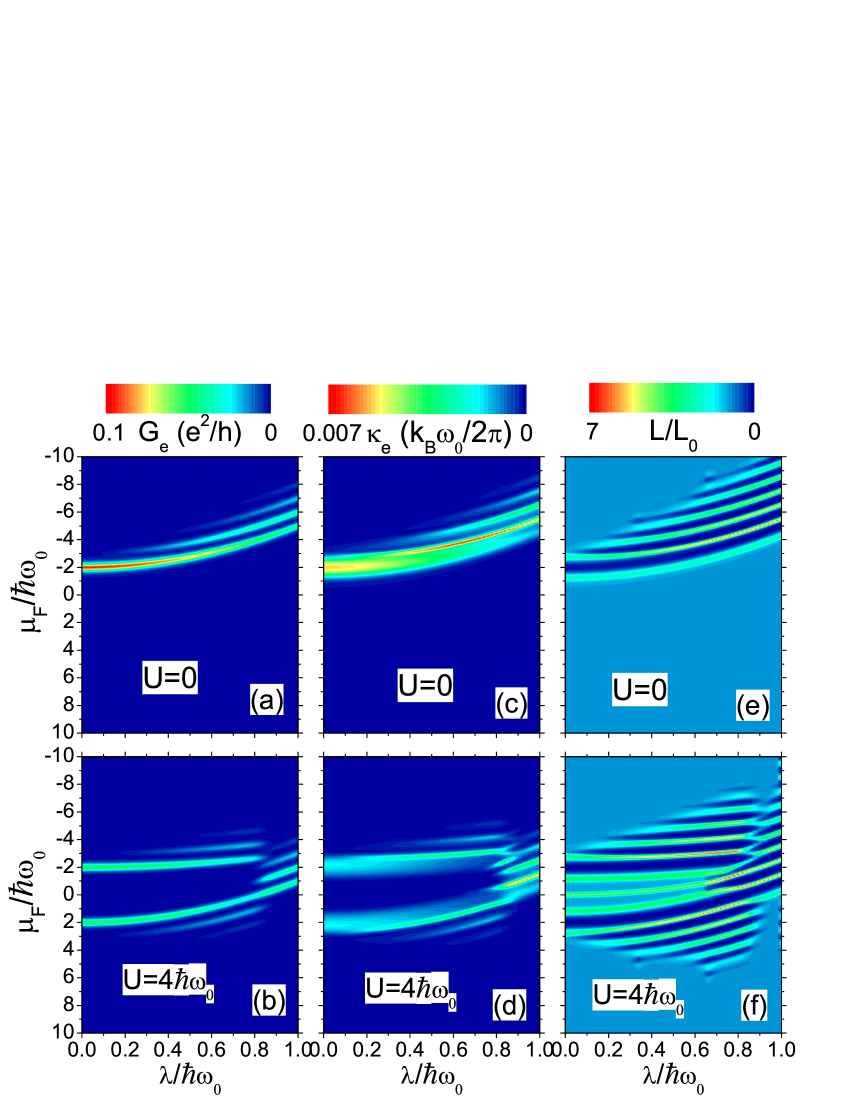
Figure 1: (Color online) Electronic and thermal conductances and Lorenz ratio as a function of $\mu_{F}$ for different e-ph and e-e interaction strengths: $\varepsilon_{0}=-2\hbar\omega_{0}$, $\Delta\varepsilon=0$, $\Gamma^{L}_{\sigma}=\Gamma^{R}_{\sigma}=0.05\hbar\omega_{0}$, $\hbar\omega_{0}=30$ meV, and $T=35$ K, which are typical experimental values. Paulsson05

Figures 1(a) and 1(b) show the electronic conductance $G_{e}$ as a function of $\mu_{F}$ for different values of $\lambda$ and $U$. We see that the number of resonance peaks increases as the e-ph coupling increases: Large $\lambda$ excites more phonons and enables multi-phonon-assisted tunneling. At low temperature, we can approximate $G_{e}$ as $\mathcal{T}(\mu_{F})$ since $-\partial f/\partial\omega\approx\delta(\omega-\mu_{F})$. Therefore, from Eqs. (5) and (3), the positions of the resonance peaks are determined by the poles of Green’s functions; i.e., $\mu_{F}$ of resonance positions are equal to $\Delta_{nm}^{(1)}$ or $\Delta_{nm}^{(2)}$. However, exponential functions and $D_{nm}$ in Eq. (5) weight the resonances and make the peaks unobservable for certain parameter ranges. From Eq. (5), when $U$ is so weak that $\tilde{\varepsilon}_{\sigma\bar{\sigma}}+U<\tilde{\varepsilon}_{\sigma}<0$, $\Delta^{(2)}_{nm}<0$ thus dominates the resonance peaks [see Fig. 1(a)]. While $U$ increases up to $\tilde{\varepsilon}_{\sigma\bar{\sigma}}+U>\tilde{\varepsilon}_{\sigma}$, two resonance branches, $\Delta^{(2)}_{nm}>0$ and $\Delta^{(1)}_{nm}<0$, emerge [see Fig. 1(b)]. For large $U$, when $\lambda$ increases further such that again $\tilde{\varepsilon}_{\sigma\bar{\sigma}}+U<\tilde{\varepsilon}_{\sigma}$, then $\Delta^{(2)}_{nm}<0$ redominates the resonances and two resonant branches merge together, as shown in Fig. 1(b). It is a consequence of the competition between the e-ph coupling and e-e interaction with the molecular quantum dot junction.

In Figs. 1(a) and 1(b), we also observe that increasing e-ph coupling decreases the peak value of the main resonance of $G_{e}$ but increases the values of side peaks of $G_{e}$. This occurs because $D^{2}_{00}=e^{-g^{2}}$ decreases with $g$ increasing, while for a positive integer $n$, $D^{2}_{0n}=g^{2n}e^{-g^{2}}/n!$ has the opposite tendency at $g\in[0,\sqrt{n}]$. When e-ph coupling $g$ increases further ($g>\sqrt{n}$), $D^{2}_{0n}$ decreases again so that side peak values of $G_{e}$ will be repressed by the strong e-ph scattering. Comparing Figs. 1(a) and 1(b), we further see that for the weak and moderate $\lambda$, increasing the Coulomb repulsion reduces $G_{e}$, which is a consequence of the factor $e^{-\beta U}$ in Eq. (5). While for strong e-ph coupling, the Coulomb repulsion mainly shifts the positions of the spectrum of $G_{e}$ while leaving its magnitude almost unaffected. This is because for large $\lambda$, while the resonance positions $\Delta^{(2)}_{nm}$ depend on $U$, the Green’s functions are dominated by $D_{nm}$, which, however, is $U$ independent.

The $\lambda$ and $U$ dependence of thermal conductance $\kappa_{e}$ is similar to that of $G_{e}$, as shown in Figs. 1(c) and 1(d). We note that the resonance positions of $\kappa_{e}$ do not coincide with those of $G_{e}$ but instead coincide with the valleys of $G_{e}$. This arrangement reflects the different ways in which the inelastic scattering induced by e-ph coupling and e-e interaction degrade heat and electrical currents. In fact, around the resonances of $G_{e}$, from Eq. (13) it is clear that $\mathcal{L}_{1,2}\simeq 0$, so we have small values of $\kappa_{e}$ from the definition Eq. (12). As a consequence, we obtain the strong violation of WF law $L/L_{0}\ll 1$ around the resonance points of $G_{e}$ [see Figs. 1(e) and 1(f)].

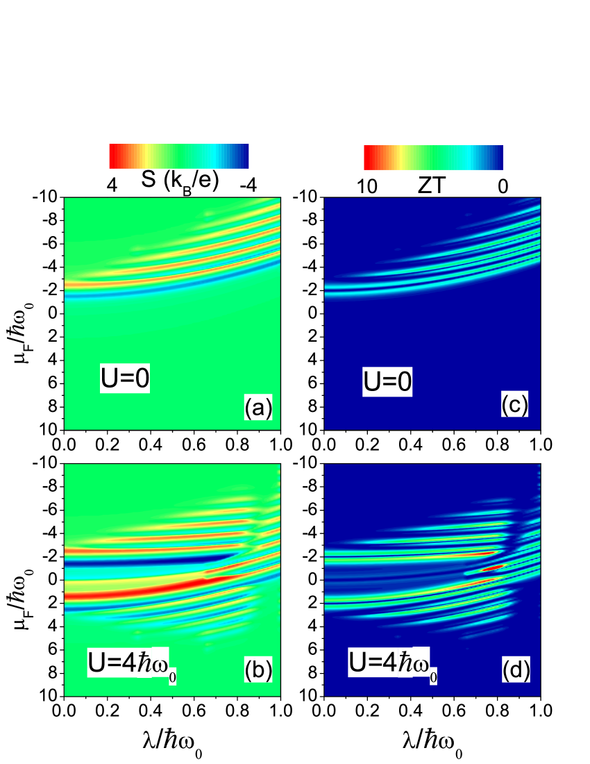
Figure 2: (Color online) $S$ and $ZT$ as a function of $\mu_{F}$ for different $\lambda$ and $U$. The Hamiltonian parameters are the same as those in Fig. 1.

Because $ZT=S^{2}/L$ becomes large as the Lorenz ratio goes to zero while the thermopower remains finite, we expect large $ZT$ peaks will emerge around the resonance points of $G_{e}$. However, as shown in Fig. 2, large $ZT$ occurs only at the sides of the resonances and drops back to zero dramatically at exact resonance positions. This occurs because the particle-hole symmetry at the resonances [$\mathcal{L}_{1}\simeq 0$ from the definition Eq. (13)] zeros the thermopower [$S\simeq 0$ from the definition Eq. (11)]. Moreover, increasing $\lambda$ increases $ZT$ as well as the number of $ZT$ peaks, which shows that large $ZT$ is favored by multi-phonon-assisted tunneling. In addition, the Coulomb repulsion increases $ZT$ such that optimal $ZT$ is obtained at the merging regime of two resonant branches, which is a consequence of the competition of e-ph coupling and Coulomb repulsion. In other words, the optimal $ZT$ is located at $\tilde{\varepsilon}_{\sigma\bar{\sigma}}+U=\tilde{\varepsilon}_{\sigma}$ as we discussed above in Figs. 1(a) and 1(b). Taking $\varepsilon_{\sigma}=\varepsilon_{\bar{\sigma}}=-2\hbar\omega_{0},U=4\hbar\omega_{0}$ as in Fig. 1(b), we then can predict that the optimal $ZT$ can occur when we choose $\lambda_{\sigma}=\sqrt{2/3}\hbar\omega_{0}\approx 0.81\hbar\omega_{0}$, which is indeed the case shown in Fig. 2(d). In turn, given the molecular level energy and the e-ph coupling strength, we also can choose a proper e-e repulsion strength $U$ to optimize the efficiency of thermoelectricity.

Finally, the temperature dependence of $ZT$ is illustrated in Fig. 3. Interestingly, we see that increasing $T$ first decreases and then increases $ZT$. Coulomb repulsion enhances $ZT$ at low temperature but suppresses it at room temperature. Nevertheless, $ZT$ remains large. This result indicates a great potential for single molecular junctions as good thermoelectric devices over a wide range of temperatures.

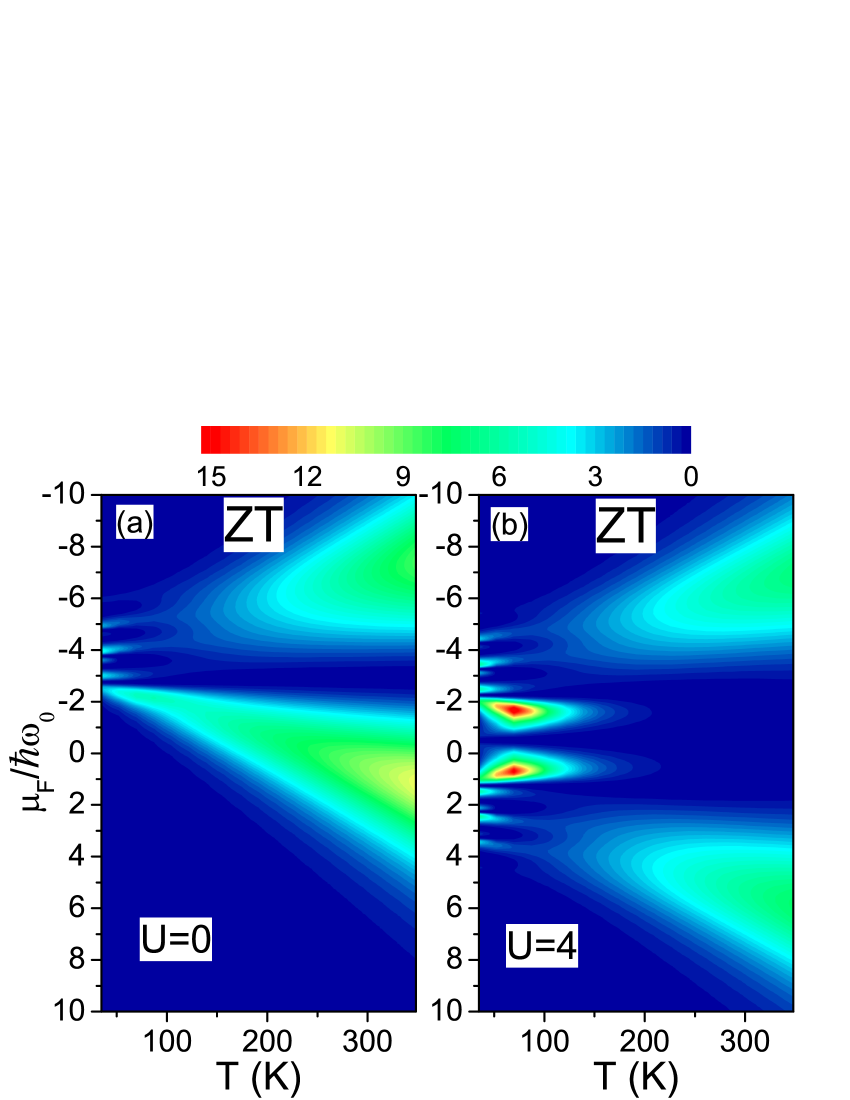
Figure 3: (Color online) Temperature-dependence of $ZT$ for moderate $\lambda=0.5\hbar\omega_{0}$, with (a) $U=0$ and (b) $U=4\hbar\omega_{0}$. Other parameters are the same as those in Fig. 1.

In view of the substantial progress that has been made in the area of molecular devices, NJTao:2006 the findings in the present work will open a new avenue for using molecular junctions for the optimal design of efficient energy conversion devices. To experimentally observe the predicted $ZT$ enhancement, the molecular junction should be gated to tune the conduction electron density. Additionally, there is also the flexibility of adjusting the coupling geometry between molecule and leads.

IV Conclusions

In conclusion, by a transformation of the phonon basis we were able to nonperturbatively deal with the molecular quantum dot for arbitrary e-ph coupling and e-e interaction strengths. After analytically calculating its Green’s functions, we coupled the molecular quantum dot to the electrode leads in the weak tunneling limit, and then computed the thermoelectric transport properties numerically. We studied the synergistic effect of e-ph and e-e interactions and showed that at low temperatures large $ZT$ occurs at the sides of resonances in electronic conductance but drops dramatically to zero at resonance. We found that increasing e-ph and e-e interactions increases $ZT$, although with $G_{e}$ repressed. In particular, large $ZT$ is favored by multi-phonon-assisted tunneling. More interestingly, we found that an optimal $ZT$ emerges when these two interactions were competing. Finally, we showed that a large $ZT$ can be obtained in a wide range of temperatures.

It would be interesting to consider the Zeeman splitting of the molecular orbital energies produced, for example, by an external magnetic field or ferromagnetic leads. Spin-related thermoelectric effects may aid the optimal design of novel thermal-spintronic devices and single-molecule-magnet junctions. Dubi09Wang10 Extending our nonperturbative approach to electronic coupling to multiple vibrational modes Hartle09 will be an interesting topic. It would also be desirable to combine the present method with some ab initio electron structure theory, like the density functional theory within the local density approximations, for more realistic calculations. Haugbook Finally, we would like to remark that calculating the exact self-energy $\Sigma_{\mathrm{lead}}$ remains an important open question, which deserves investigation in the future.

Appendix A Calculation details of nonequilibrium Green’s functions

Before calculating the retarded (advanced) Green’s function, we first detail the calculation of the lesser Green’s function $G_{\sigma}^{<}(t)=i\langle d^{{\dagger}}_{\sigma}(0)d_{\sigma}(t)\rangle$ in the frequency domain:

$$G_{\sigma}^{<}(\omega)= i\int^{+\infty}_{-\infty}dte^{i\omega t}\langle d_{\sigma}^{{\dagger}}(0)d_{\sigma}(t)\rangle$$

$$= i\int^{+\infty}_{-\infty}dte^{i\omega t}\sum_{\varphi}\sum_{\psi}\langle\varphi|\rho d_{\sigma}^{{\dagger}}(0)|\psi\rangle$$

$$\times\langle\psi|e^{iH_{\mathrm{mol}}t}d_{\sigma}(0)e^{-iH_{\mathrm{mol}}t}|\varphi\rangle$$

$$= \frac{i}{Z}\int^{+\infty}_{-\infty}dte^{i\omega t}\sum_{\varphi}\sum_{\psi}e^{-\beta E_{\varphi}}e^{-i(E_{\varphi}-E_{\psi})t}$$

$$\times\langle\varphi|d_{\sigma}^{{\dagger}}(0)|\psi\rangle\langle\psi|d_{\sigma}(0)|\varphi\rangle$$

$$= \frac{2\pi i}{Z}\sum_{\varphi}\sum_{\psi}\delta(\omega-(E_{\varphi}-E_{\psi}))e^{-\beta E_{\varphi}}$$

$$\times\langle\varphi|d_{\sigma}^{{\dagger}}(0)|\psi\rangle\langle\psi|d_{\sigma}(0)|\varphi\rangle,$$ (14)

where we used $\rho=e^{-\beta H_{\mathrm{mol}}}/Z$ with $Z=\text{Tr}(e^{-\beta H_{\mathrm{mol}}})=(1+N_{\mathrm{ph}})(1+e^{-\beta\tilde{\varepsilon}_{\sigma}}+e^{-\beta\tilde{\varepsilon}_{\bar{\sigma}}}+e^{-\beta(\tilde{\varepsilon}_{\sigma\bar{\sigma}}+U)})$ and $N_{\mathrm{ph}}$ is the Bose distribution $N_{ph}=1/(e^{\beta\omega_{0}}-1)$. Here $|\varphi\rangle$ and $|\psi\rangle$ are the possible eigenstates $|\o,n\rangle_{\o}$, $|\sigma,n\rangle_{\sigma}$, $|\bar{\sigma},n\rangle_{\bar{\sigma}}$, $|\sigma\bar{\sigma},n\rangle_{\sigma\bar{\sigma}}$, and $E_{\varphi}$ and $E_{\psi}$ are the corresponding possible eigenvalues $n\omega_{0}$, $n\omega_{0}+\tilde{\varepsilon}_{\sigma}$, $n\omega_{0}+\tilde{\varepsilon}_{\bar{\sigma}}$, $n\omega_{0}+\tilde{\varepsilon}_{\sigma\bar{\sigma}}+U$.

There are only two nonzero combinations of $|\varphi\rangle$ and $|\psi\rangle$ for calculating $G_{\sigma}^{<}(\omega)$: (1) $|\varphi\rangle=|\sigma,n\rangle_{\sigma}$ and $|\psi\rangle=|\o,m\rangle_{\o}$, or (2) $|\varphi\rangle=|\sigma\bar{\sigma},n\rangle_{\sigma\bar{\sigma}}$ and $|\psi\rangle=|\bar{\sigma},m\rangle_{\bar{\sigma}}$, such that the lesser Green’s function can be reduced to

$$G_{\sigma}^{<}(\omega)= \frac{2\pi i}{Z}\sum^{\infty}_{n=0}\sum^{\infty}_{m=0}\big{[}\delta(\omega-(n-m)\omega_{0}-\tilde{\varepsilon}_{\sigma})$$

$$\times e^{-\beta(n\omega_{0}+\tilde{\varepsilon}_{\sigma})}{{}_{\sigma}\langle}n|m\rangle_{\o}\;{{}_{\o}\langle}m|n\rangle_{\sigma}$$

$$+\delta(\omega-(n-m)\omega_{0}-(\tilde{\varepsilon}_{\sigma\bar{\sigma}}-\tilde{\varepsilon}_{\bar{\sigma}}+U))$$

$$\times e^{-\beta(n\omega_{0}+\tilde{\varepsilon}_{\sigma\bar{\sigma}}+U)}{{}_{\sigma\bar{\sigma}}\langle}n|m\rangle_{\bar{\sigma}}\;{{}_{\bar{\sigma}}\langle}m|n\rangle_{\sigma\bar{\sigma}}\big{]}.$$ (15)

The detailed expression of ${{}_{b}\langle}n|m\rangle_{c}$, denoting the inner product of modified phonon states with effective displacements $g_{b}$ and $g_{c}$, can be derived as follows:

$${{}_{b}\langle}n|m\rangle_{c} = \langle 0|\frac{(\hat{a}+g_{b})^{n}}{\sqrt{n!}}\exp{(-{g_{b}}^{2}/2-g_{b}\hat{a})}$$ (16)

$$\times\frac{(\hat{a}^{{\dagger}}+g_{c})^{m}}{\sqrt{m!}}\exp{(-{g_{c}}^{2}/2-g_{c}\hat{a}^{{\dagger}})}|0\rangle$$

$$= \frac{\exp{[-(g_{b}-g_{c})^{2}/2]}}{\sqrt{n!m!}}$$

$$\times\langle 0|(\hat{a}+g_{b})^{n}e^{(-g_{c}\hat{a}^{{\dagger}})}e^{(-g_{b}\hat{a})}(\hat{a}^{{\dagger}}+g_{c})^{m}|0\rangle$$

$$= \frac{\exp{[-(g_{b}-g_{c})^{2}/2]}}{\sqrt{n!m!}}$$

$$\times\langle 0|(\hat{a}+g_{b}-g_{c})^{n}(\hat{a}^{{\dagger}}+g_{c}-g_{b})^{m}|0\rangle$$

$$= \frac{\exp{[-(g_{b}-g_{c})^{2}/2]}}{\sqrt{n!m!}}$$

$$\times\sum^{\mathrm{min}\{n,m\}}_{k=0}k!C^{k}_{n}(g_{b}-g_{c})^{n-k}C^{k}_{m}(g_{c}-g_{b})^{m-k}$$

$$= (-1)^{m}D_{nm}(g_{b}-g_{c})$$

where

$$D_{nm}(x)=e^{-x^{2}/2}\sum^{\mathrm{min}\{n,m\}}_{k=0}\frac{(-1)^{k}\sqrt{n!m!}x^{n+m-2k}}{(n-k)!(m-k)!k!}$$

is invariant under the exchange of indices $n,m$. Note, to get the third equivalence, we utilized the relation $\exp{(c\hat{a})}f(\hat{a}^{{\dagger}},\hat{a})=f(\hat{a}^{{\dagger}}+c,\hat{a})\exp{(c\hat{a})}$.

Therefore, the lesser Green’s function can be further reduced:

$$G_{\sigma}^{<}(\omega)=\frac{2\pi i}{Z}\sum^{\infty}_{n,m=0}\left[\delta(\omega-\Delta_{nm}^{(1)})e^{-\beta(n\omega_{0}+\tilde{\varepsilon}_{\sigma})}+\right.$$

$$\left.\delta(\omega-\Delta_{nm}^{(2)})e^{-\beta(n\omega_{0}+\tilde{\varepsilon}_{\sigma\bar{\sigma}}+U)}\right]D^{2}_{nm}(g_{\sigma}),$$ (17)

where

$$\Delta_{nm}^{(1)} = (n-m)\omega_{0}+\tilde{\varepsilon}_{\sigma},$$ (18)

$$\Delta_{nm}^{(2)} = (n-m)\omega_{0}+(\tilde{\varepsilon}_{\sigma}-2\omega_{0}g_{\sigma}g_{\bar{\sigma}}+U).$$ (19)

Similarly, for the greater Green’s function $G^{>}_{\sigma}(t)=-i\langle d_{\sigma}(t)d^{{\dagger}}_{\sigma}(0)\rangle$, we can obtain

$$G_{\sigma}^{>}(\omega) = -i\int dte^{i\omega t}\langle d_{\sigma}(t)d_{\sigma}^{{\dagger}}(0)\rangle$$ (20)

$$= -i\int dte^{i\omega t}\sum_{\varphi}\sum_{\psi}\langle\varphi|\rho e^{iH_{\mathrm{mol}}t}d_{\sigma}(0)e^{-iH_{\mathrm{mol}}t}|\psi\rangle$$

$$\times\langle\psi|d_{\sigma}^{{\dagger}}(0)|\varphi\rangle$$

$$= -\frac{2\pi i}{Z}\sum_{\varphi}\sum_{\psi}\delta(\omega+E_{\varphi}-E_{\psi})e^{-\beta E_{\varphi}}$$

$$\times\langle\varphi|d_{\sigma}|\psi\rangle\langle\psi|d_{\sigma}^{{\dagger}}|\varphi\rangle$$

$$= -\frac{2\pi i}{Z}\sum_{n,m}\left[\delta(\omega-\Delta_{nm}^{(1)})e^{-\beta m\omega_{0}}+\right.$$

$$\left.\delta(\omega-\Delta_{nm}^{(2)})e^{-\beta(m\omega_{0}+\tilde{\varepsilon}_{\bar{\sigma}})}\right]D^{2}_{nm}(g_{\sigma}).$$

Note here the two nonzero combinations of $|\varphi\rangle$ and $|\psi\rangle$ for calculating $G_{\sigma}^{>}(\omega)$ are (1) $|\varphi\rangle=|\o,m\rangle_{\o}$ and $|\psi\rangle=|\sigma,n\rangle_{\sigma}$, or (2) $|\varphi\rangle=|\bar{\sigma},m\rangle_{\bar{\sigma}}$ and $|\psi\rangle=|\sigma\bar{\sigma},n\rangle_{\sigma\bar{\sigma}}$.

Then, following the relation $G^{r}(t)=\Theta(t)(G^{>}(t)-G^{<}(t))$, $G^{a}(t)=-\Theta(-t)(G^{>}(t)-G^{<}(t))$, and utilizing

$$\Theta(t)=\int\frac{d\omega}{2\pi i}\frac{e^{i\omega t}}{\omega-i0^{+}},$$

we have the retarded (advanced) Green’s function:

$$G_{\sigma}^{r(a)}(\omega) = \int\frac{d\omega_{1}}{2\pi}\int\frac{d\omega_{2}}{2\pi i}\int dte^{i\omega t}\frac{e^{-i(\omega_{1}-\omega_{2})t}}{\omega_{2}\mp i0^{+}}$$ (21)

$$\times[G_{\sigma}^{>}(\omega_{1})-G_{\sigma}^{<}(\omega_{1})]$$

$$= \int\frac{d\omega_{1}}{2\pi i}\frac{G_{\sigma}^{>}(\omega_{1})-G_{\sigma}^{<}(\omega_{1})}{\omega_{1}-\omega\mp i0^{+}}.$$

Substituting the expressions of the greater and lesser Green’s functions, we arrive at Eq. (5).

Appendix B Derivations for the current expression

Here we detail the calculation of the current through the interacting system. The electronic current from left contact to central system is defined as $J_{L}=-e\langle\sum_{k\sigma}{dN^{L}_{k\sigma}}/{dt}\rangle$, which is generally reexpressed as Haugbook

$$J_{L}=\frac{ie}{\hbar}\int\frac{d\omega}{2\pi}\sum_{\sigma}\left[\Gamma_{\sigma}^{L}G^{<}_{\mathrm{tot},\sigma}+\Gamma_{\sigma}^{L}f_{L}(G^{r}_{\mathrm{tot},\sigma}-G^{a}_{\mathrm{tot},\sigma})\right].$$ (22)

Substituting the expressions of various nonequilibrium Green’s functions,

$$G^{r(a)}_{\mathrm{tot},\sigma} = \frac{1}{(G^{r(a)}_{\sigma})^{-1}\pm i\Gamma_{\sigma}},$$ (23)

$$G^{<(>)}_{\mathrm{tot},\sigma} = G^{r}_{\mathrm{tot},\sigma}\Sigma^{<(>)}_{\mathrm{tot},\sigma}G^{a}_{\mathrm{tot},\sigma},$$ (24)

we have

$$J_{L} = \frac{ie}{\hbar}\int\frac{d\omega}{2\pi}\sum_{\sigma}[\Gamma_{\sigma}^{L}G^{<}_{\mathrm{tot},\sigma}+\Gamma_{\sigma}^{L}f_{L}(G^{r}_{\mathrm{tot},\sigma}-G^{a}_{\mathrm{tot},\sigma})]$$ (25)

$$= \frac{ie}{\hbar}\int\frac{d\omega}{2\pi}\sum_{\sigma}\frac{\Gamma^{L}_{\sigma}(\Sigma^{<}_{\mathrm{lead},\sigma}+\Sigma^{<}_{\mathrm{int},\sigma})-(2i\Gamma_{\sigma}+(G^{r}_{\sigma})^{-1}-(G^{a}_{\sigma})^{-1})\Gamma_{\sigma}^{L}f_{L}}{[(G^{r}_{\sigma})^{-1}+i\Gamma_{\sigma}][(G^{a}_{\sigma})^{-1}-i\Gamma_{\sigma}]}$$ (26)

$$= \frac{ie}{\hbar}\int\frac{d\omega}{2\pi}\sum_{\sigma}\frac{\Gamma^{L}_{\sigma}\Sigma^{<}_{\mathrm{lead},\sigma}-2i\Gamma_{\sigma}\Gamma_{\sigma}^{L}f_{L}}{[(G^{r}_{\sigma})^{-1}+i\Gamma_{\sigma}][(G^{a}_{\sigma})^{-1}-i\Gamma_{\sigma}]}+\frac{ie}{\hbar}\int\frac{d\omega}{2\pi}\sum_{\sigma}\frac{\Gamma^{L}_{\sigma}G^{<}_{\sigma}+\Gamma_{\sigma}^{L}f_{L}(G^{r}_{\sigma}-G^{a}_{\sigma})}{[1+i\Gamma_{\sigma}G^{r}_{\sigma}][1-i\Gamma_{\sigma}G^{a}_{\sigma}]}$$ (28)

$$= \frac{e}{\hbar}\int\frac{d\omega}{2\pi}\sum_{\sigma}\frac{\Gamma^{L}_{\sigma}\Gamma^{R}_{\sigma}}{[(G^{r}_{\sigma})^{-1}+i\Gamma_{\sigma}][(G^{a}_{\sigma})^{-1}-i\Gamma_{\sigma}]}\big{[}f_{L}(\omega)-f_{R}(\omega)\big{]}$$

$$+\frac{ie}{\hbar}\int\frac{d\omega}{2\pi}\sum_{\sigma}\frac{\Gamma^{L}_{\sigma}G^{<}_{\sigma}+\Gamma_{\sigma}^{L}f_{L}(G^{>}_{\sigma}-G^{<}_{\sigma})}{[1+i\Gamma_{\sigma}G^{r}_{\sigma}][1-i\Gamma_{\sigma}G^{a}_{\sigma}]}$$

In the integration of the last line, the lesser and greater Green’s functions contain the Dirac $\delta$ functions, which only have finite nonzero values at the resonant points. However, at those resonant points, the retarded and advanced Green’s functions have divergent values, which finally lead to zero integration values. Therefore, the contribution of the last integration is zero, and we finally arrive at the electron current expression, Eq. (6). It is easy to get the same expression for $J_{R}$ with $R\leftrightarrow L$, such that current conservation is explicitly preserved.

Following the first law of thermodynamics $dQ=dE-\mu dN$, we have the current relation: $I_{Q}\equiv\dot{Q}=\dot{E}-\mu J$. Therefore, following the similar calculation, the heat current is straightforwardly obtained as Eq. (7). We can obtain the similar expression for the heat current through the right reservoir $I^{R}_{Q}$. Based on the electron current expression and the expression of heat current carried by the electron, we are capable of investigating the thermoelectric transport properties.

References

(1) G. J. Snyder and E. R. Toberer, Nat. Mater. 7, 105 (2008).
(2) M. S. Dresselhaus et al., Adv. Mater. 19, 1043 (2007).
(3) A. Majumdar, Science 303, 777 (2004).
(4) G. D. Mahan and J. O. Sofo, Proc. Natl Acad. Sci. USA 93, 7436 (1996).
(5) Y. Dubi and M. Di Ventra, Rev. Mod. Phys. 83, 131 (2011).
(6) P. Reddy et al., Science, 316, 1568 (2007).
(7) J. Park et al., Nature 417, 722 (2002); W. Liang
et al, Nature 417, 725 (2002).
(8) M. Galperin, M. A. Ratner, and A. Nitzan, J. Phys.: Condens. Matter 19, 103201 (2007).
(9) H. Haug and A. P. Jauho, Quantum Kinetics in Transport and Optics of Semiconductors (Springer-Verlag, Berlin, 2008).
(10) P. Murphy, S. Mukerjee, and J. Moore, Phys. Rev. B 78,
161406(R) (2008).
(11) T. A. Costi and V. Zlatić, Phys. Rev. B 81, 235127 (2010).
(12) J. Liu, Q.-F. Sun, and X. C. Xie, Phys. Rev. B 81, 245323 (2010).
(13)Karol Izydor Wysokiński, Phys. Rev. B 82, 115423 (2010).
(14) O. Entin-Wohlman, Y. Imry, and A. Aharony, Phys.
Rev. B 82, 115314 (2010).
(15) X. Zianni, Phys. Rev. B 82, 165302 (2010).
(16) J. Koch, F. von Oppen, Y. Oreg and E. Sela, Phy. Rev. B 70, 195107 (2004).
(17) M. Leijnse, M. R. Wegewijs, and K. Flensberg,
Phys. Rev. B 82, 045412 (2010).
(18) M. Paulsson, T. Frederiksen, and M. Brandbyge,
Phys. Rev. B 72, 201101(R) (2005).
(19) F. Haupt, T. Novotný, and W. Belzig, Phys. Rev.
Lett. 103, 136601 (2009); T. L. Schmidt and A. Komnik, Phys.
Rev. B 80, 041307(R) (2009); R. Avriller and A. Levy Yeyati,
Phys. Rev. B 80, 041309(R) (2009).
(20) J.-X. Zhu and A. V. Balatsky, Phys. Rev. B 67, 165326
(2003); Z.-Z. Chen, R. Lü, and B.-F. Zhu, Phys. Rev. B 71,
165324 (2005).
(21) G. D. Mahan, Many-Particle Physics (New York, 1990).
(22) D. M.-T. Kuo, Jpn. J. Appl. Phys. 49, 095205 (2010).
(23) T. Holstein, Ann. Phys. (NY) 8, 325 (1959).
(24) A. C. Hewson and D. Meyer, J. Phys. Condens. Matter 14, 427 (2002).
(25) Q. H. Chen, Y. Y. Zhang, T. Liu, and K. L. Wang, Phys. Rev.
A 78, 051801 (2008).
(26) C. Wang, J. Ren, B. Li, and Q. H. Chen, arXiv:1101.4864, to appear in Eur. Phys. J. B.
(27) A. Martin-Rodero, A. Levy Yeyati, F. Flores, and R. C. Monreal, Phys. Rev. B 78, 235112 (2008).
(28) S. Maier, T. L. Schmidt, and A. Komnik, Phys. Rev. B 83, 085401 (2011).
(29) J. T. Lü and J.-S. Wang, Phys. Rev. B 76, 165418 (2007).
(30) B. Kubala, J. König, and J. Pekola, Phys. Rev.
Lett. 100, 066801 (2008).
(31) Y. Dubi and M. Di Ventra, Phys. Rev. B 79, 081302(R)
(2009); R.-Q. Wang, L. Sheng, R. Shen, B. Wang, and D. Y. Xing,
Phys. Rev. Lett. 105, 057202 (2010).
(32) N. J. Tao, Nature Nanotech. 1, 173 (2006).
(33) R. Härtle, C. Benesch, and M. Thoss, Phys. Rev. Lett. 102, 146801 (2009).