Opportunistic Power Control for Multi-Carrier Interference Channels

Abstract

We propose a new method for opportunistic power control in multi-carrier interference channels for delay-tolerant data services. In doing so, we utilize a game theoretic framework with novel constraints, where each user tries to maximize its utility in a distributed and opportunistic manner, while satisfying the game’s constraints by adapting its transmit power to its channel. In this scheme, users transmit with more power on good sub-channels and do the opposite on bad sub-channels. In this way, in addition to the allocated power on each sub-channel, the total power of all users also depends on channel conditions. Since each user’s power level depends on power levels of other users, the game belongs to the generalized Nash equilibrium (GNE) problems, which in general, is hard to analyze. We show that the proposed game has a GNE, and derive the sufficient conditions for its uniqueness. Besides, we propose a new pricing scheme for maximizing each user’s throughput in an opportunistic manner under its total power constraint; and provide the sufficient conditions for the algorithm’s convergence and its GNE’s uniqueness. Simulations confirm that our proposed scheme yields a higher throughput for each user and/or has a significantly improved efficiency as compared to other existing opportunistic methods.

I Introduction

Frequency spectrum of a network can be divided into many orthogonal sub-channels that can be shared by all users. However, shared usage of spectrum by a user produces interference to other users. As the number of users increases, users’ received interference levels increase as well, resulting in fewer users that can achieve their required quality of service (QoS). In such instances, efficient use of spectrum becomes more important, meaning that users should transmit at their lowest possible power levels while satisfying their required data rates.

Radio resource allocation in multi-carrier wireless networks aims to allocate available resources to users in such a way that under some system and service constraints, a performance measure for each user, e.g., the total throughput or the total transmit power, is optimized. In distributed resource allocation, each user chooses its strategy (required resources) independent of other users. Game theory [1] is commonly used in the literature to analyze distributed resource allocation algorithms by formulating the problem as a non-cooperative game, where each user competes with other users with a view to optimizing its own utility. The game settles at its Nash equilibrium (NE), where no user can improve its utility by unilaterally changing its strategy.

In the context of distributed resource allocation, the problem of power minimization under throughput constraint is considered in [2, 3]. In this problem, each user tries to minimize its total consumed power over all sub-channels while maintaining its total throughput above a predefined threshold. In such a game, since the strategy space of each user depends on the chosen strategies of other users, the game cannot be analyzed by way of the conventional Nash equilibrium, and the so called generalized Nash equilibrium (GNE) should be used [4]. In [2], the game is simulated, and in [3], the game is mathematically analyzed and the sufficient conditions for the existence and uniqueness of GNE, as well as the sufficient conditions for the convergence of the distributed algorithm are presented.

The counterpart of this problem in single carrier systems is known as the target SINR-tracking power-control algorithm (TPC) [5]. In TPC, each user tries to choose its transmit power in a distributed manner with a view to satisfying its predefined target SINR. An important issue in TPC is its feasibility, meaning that the algorithm converges only if a power vector exists such that the target SINRs of all users are satisfied. In TPC, users adapt their transmit power levels to their channel conditions, i.e., each user increases its transmit power when its channel is bad, and does the reverse when its channel is good. Likewise, minimizing the transmit power under the data rate constraint may not be feasible, as there may not be a power vector that satisfies the data rate constraints for all users, meaning that no GNE may exist. Also, since users consume more power when their channels are bad, they increase their interference to others, which in turn forces others to increase their transmit power levels, and thus aggravating the situation further for all users.

To avoid such a case for delay-tolerant services, it is worthwhile for users to reduce their transmit power (which would result in lower data rates) when their channels are bad, and do the reverse when their channels are good. This is the opportunistic power control (OPC) that was introduced and analyzed in [6] for single carrier systems. The alternative OPC for multi-carrier systems is that users try to maximize their total throughput over all sub-channels in a distributed manner when the total transmit power for each user is constrained. This game has been extensively analyzed in [7, 8, 9, 10, 11], and different conditions for the uniqueness of NE and for the convergence of the distributed algorithms are obtained. The drawbacks of this scheme include causing interference without any gain by a transmitting user when its channel is bad, and convergence to an inefficient NE because of self-serving and independent users.

In [7], the data rate maximization game is analyzed and the sufficient conditions for NE’s uniqueness are obtained. In addition, by interpreting the waterfilling solution as a projector and using its contraction property [12], in [8, 9], the sufficient conditions for the convergence of the iterative waterfilling solution are derived. Using linear complementarity [10] reformulation of the Karush-Kuhn-Tucker (KKT) condition [13] of the rate maximization game, in [14], the linear complementarity conditions are converted to the affine variational inequality [15], and the sufficient conditions for NE’s uniqueness and convergence of the iterative waterfilling algorithm are obtained. In [11], the sufficient conditions for NE’s uniqueness and convergence of the iterative waterfilling algorithm are established by interpreting the waterfilling solution as a piecewise affine function [15].

In a non-cooperative game, since each user selfishly tries to optimize its own utility, the equilibrium of the game may not be a desirable one. In such cases, pricing is an effective mechanism to control users’ behaviors and achieve a more efficient NE. The proposed pricing in [16, 17] for the rate maximization game is a linear function of the transmit power. In [16], only numerical results are presented that provide some insight on NE’s uniqueness and convergence of the distributed algorithm, whereas in [17], a mathematical analysis based on the notion of variational inequalities and non-linear complementarity is presented to obtain the sufficient conditions for NE’s existence and for convergence of the distributed algorithm.

In this paper, we propose an OPC for multi-carrier interference channels using a game theoretic framework. In our scheme, each user opportunistically tries to maximize its total transmit power over all sub-channels in a distributed manner with a view to maximizing its data rate while satisfying the given constraint on the total transmit power that depends on interference levels in sub-channels. In doing so, higher transmit power levels are allocated to sub-channels with low interference, and lower power levels to high interference sub-channels. This is in contrast to the rate maximization game with total power constraint irrespective of interference levels on sub-channels [2, 14].

For the proposed game, we analyze the existence of GNE. Similar to the power minimization game with data rate constraint, the strategy space of a user in our proposed scheme depends on the strategies chosen by other users. However, we will show that at least one GNE is guaranteed to exist for the proposed scheme. In addition, we obtain the sufficient conditions for GNE’s uniqueness, and for the convergence of the distributed algorithm. We also introduce pricing to the rate maximization game for controlling selfish users and providing incentives for behaving in an opportunistic manner. In doing so, pricing is a function of the user’s transmit power and the interference experienced by that user. Furthermore, we obtain the sufficient conditions for NE’s uniqueness, and for the the distributed algorithm’s convergence by utilizing variational inequalities as in [14, 3, 8, 17]. By way of simulation, we evaluate the performance of our proposed OPC, as well as that of the pricing-based data rate maximization problem, and show that the total throughput of users is increased as compared to when pricing is not applied.

This paper is organized as follows. A brief review of the TPC and the OPC algorithms is provided in Section II. The opportunistic power control problem is studied in Section III, and our pricing is introduced in Section IV. Simulation results are presented in Section V, and conclusions are in Section VI.

II TPC and OPC in Single Carrier Systems

Consider a single carrier wireless network with $M$ active users that are spread in its coverage area. Let the channel gain between the transmitter of user $j$ and the receiver of user $i$ be $G_{i,j}$, and noise power at the receiver of user $i$ be $\eta_{i}$. When user $i$ transmits at power level $p_{i}$, its SINR, denoted by $\gamma_{i}$ is

$$\gamma_{i}=\frac{{G_{i,i}}{p_{i}}}{\sum\limits_{j\neq i}{{G_{i,j}}{p_{j}}}+\eta_{i}}.$$ (1)

We denote the effective interference by

$$I_{i}=\frac{\sum\limits_{j\neq i}{{G_{i,j}}{p_{j}}}+\eta_{i}}{G_{i,i}}.$$ (2)

The value of $I_{i}$ depends on power levels of users (i.e., $I_{i}(\textbf{p})$), but for simplicity in notation, we use $I_{i}$.

Consider a case in which each user chooses its power level in a distributed and iterative manner with a view to maintaining its SINR above a predefined threshold, i.e., $\gamma_{i}\geq\hat{\gamma}_{i}$. In this case, a distributed algorithm for achieving a given fixed target SINRs (TPC) as in [5] is

$$p_{i}(n+1)=\frac{\hat{\gamma}_{i}}{\gamma_{i}(n)}p_{i}(n).$$ (3)

When the system is feasible, i.e., if there exists a power vector $\textbf{p}=[p_{1},\cdots,p_{M}]$ such that the SINR constraints are satisfied, this algorithm converges to the solution of the following problem

$$\text{min}\sum p_{i}$$

$$\text{subject to:}~{}\gamma_{i}\geq\hat{\gamma}~{}\qquad\forall i,$$

where all constraints are satisfied with the equality.

To maintain a predefined SINR, a user with a bad channel transmits at high power and causes interference to other users with no apparent benefit to itself. To increase the system throughput, for delay-tolerant services, it is better that users with bad channels reduce their transmit power even to 0, and users with good channels do the reverse, and both groups adapt their data rates to their respective transmit power levels. This is the OPC algorithm, defined by

$$p_{i}(n+1)=\frac{\zeta_{i}}{I_{i}(n)},$$ (5)

where $\zeta_{i}$ is a predefined constant and $I_{i}(n)$ is the effective interference experienced by user $i$ in iteration $n$ as defined in (2). As such, each user transmits at a rate given by

$$R_{i}=\log(1+\gamma_{i}),$$ (6)

where $\gamma_{i}$ is defined in (1). From (5), it is clear that when the channel is bad, i.e., when $I_{i}$ is high, the user decreases its transmit power, and when the channel is good, i.e., when $I_{i}$ is low, it does the opposite. For a given transmit power level, the OPC’s throughput is higher than that of TPC.

III Opportunistic Power Control

III-A Problem Formulation

We now formulate the opportunistic power control problem for multi-carrier interference channels via a game theoretic framework. We begin by considering a special power control problem that is the TPC’s counterpart in multi-carrier systems. In this problem, each user tries to minimize its total transmit power over all sub-channels in a distributed manner, while maintaining its total data rate above a given threshold $\hat{R}_{i}$. This problem is stated by

$$\min_{\textbf{p}_{i}\geq 0}~{}\sum\limits_{l}p_{i}^{l}$$

$$\text{subject to:}~{}\sum\log(1+\frac{{G_{i,i}^{l}}{p_{i}^{l}}}{\sum\limits_{j\neq i}{{G_{i,j}^{l}}{p_{j}^{l}}}+\eta_{i}^{l}})\geq\hat{R}_{i},$$

where $p_{i}^{l}$ is the transmit power of user $i$ over sub-channel $l$, and $G_{i,j}^{l}$ is the channel gain from the transmitter of user $i$ to the receiver of user $j$ on sub-channel $l$.

In this game, each user tries to choose an optimal power vector $\textbf{p}_{i}=[p_{i}^{1},\cdots,p_{i}^{L}]^{\text{T}}$, where $L$ is the number of sub-channels that are utilized to satisfy the data rate constraint, such that the data rate constraint in (III-A) is satisfied with the equality. Similar to TPC, in this game, a user with a bad channel increases its transmit power to satisfy its rate constraint, which can cause more interference to other users, resulting in higher transmit power levels. To make this algorithm opportunistic, we use a new constraint and reformulate the objective function. The basic idea is similar to OPC, i.e., users increase their transmit power in good sub-channels, and do the opposite in bad sub-channels, but in a more profound manner. This will lead to a higher total throughput and a lower transmit power. We first define the utility of each user $i$ as its total power over all sub-channels. In opportunistic power control for multi-carrier interference channels, each user chooses a strategy from its strategy space that maximizes its utility. In other words, each user consumes more power to achieve a higher data rate. As each user attempts to maximize its utility (its total power consumed over all sub-channels), we impose a constraint on each user’s transmit power, and provide it with incentives to behave opportunistically. One choice for the constraint would be

$$\sum\limits_{l}(p_{i}^{l}I_{i}^{l})\leq\hat{\varsigma}_{i},$$ (8)

where $\hat{\varsigma}_{i}$ is a predefined upper bound for $\sum\limits_{l}(p_{i}^{l}I_{i}^{l})$, and

$$I_{i}^{l}=\frac{\sum\limits_{j\neq i}{{G_{i,j}^{l}}{p_{j}^{l}}}+\eta_{i}^{l}}{G_{i,i}^{l}}=\sum\limits_{j\neq i}\hat{G}_{i,j}^{l}p_{j}^{l}+\hat{\eta}_{i}^{l}.$$ (9)

Note that, the value of $I_{i}^{l}$ depends on power levels of users (i.e., $I_{i}^{l}(\textbf{p})$, but for simplicity in notation, we use $I_{i}^{l}$.

Considering (8), one can observe that users would allocate more power on good sub-channels. In addition, the total power consumed by users depends on sub-channel conditions. With this constraint and the objective functions as the total power over all sub-channels, each user needs to solve a linear program in which its entire transmit power is assigned only to the best sub-channels, which causes instability in the iterative algorithm. Moreover, when effective interference levels are the same on some sub-channels, the problem would have numerous solutions. This means that the convergence analysis of this problem is very difficult, and convergence would be guaranteed in a very restrictive set of channel conditions. Due to the above problems, instead of (8), we define a new constraint for each user as

$$\sum\limits_{l}(p_{i}^{l}I_{i}^{l})^{2}\leq\varsigma_{i},$$ (10)

where $\varsigma_{i}$ is a predefined upper bound for $\sum\limits_{l}(p_{i}^{l}I_{i}^{l})^{2}$, and $I_{i}^{l}$ is defined in (9).

Similar to (8), applying the constraint (10) would cause each user to transmit at higher power levels on good sub-channels, and the total transmit power will depend on the channel conditions of sub-channels. The strategy space of each user is

$$\mathcal{P}_{i}(\textbf{p}_{-i})=\{\textbf{p}_{i}:p_{i}^{l}\geq 0,\sum\limits_{l}(p_{i}^{l}I_{i}^{l})^{2}\leq\varsigma_{i}\},$$ (11)

where $\textbf{p}_{-i}$ is the strategies of all users other than user $i$.

The problem is formulated by the game $\mathcal{G}^{\text{o}}=\langle\mathcal{M},\mathcal{P}_{i}(\textbf{p}_{-i}),\{u_{i}\}\rangle$, where $\mathcal{M}$ is the set of users in the system, $\mathcal{P}_{i}(\textbf{p}_{-i})$ is the strategy space of user $i$ defined in (11), and $u_{i}$ is the utility of user $i$. Each user aims to solve

$$\max_{\textbf{p}_{i}\geq 0}~{}\sum\limits_{l}p_{i}^{l}$$

$$\text{subject to:}~{}\textbf{p}_{i}\in\mathcal{P}_{i}(\textbf{p}_{-i}),$$

where $\mathcal{P}_{i}(\textbf{p}_{-i})$ is defined in (11).

III-B Game Analysis

In the opportunistic power control game, each user solves (III-A) in a distributed manner. Since the strategy space of user $i$, i.e., $\mathcal{P}_{i}(\textbf{p}_{-i})$, depends on the strategies of other users, this game belongs to the generalized Nash equilibrium (GNE) problems [4]. In such games, in addition to the utility function, users’ interactions affect their strategy choices. However, this dependence makes the problem hard to analyze. In what follows, we present an analysis of (III-A). When users iteratively solve (III-A), the game settles at a GNE as defined below.

Definition 1: The strategy vector $\textbf{p}=[\textbf{p}_{1}^{\text{*T}},\cdots,\textbf{p}_{M}^{\text{*T}}]^{\text{T}}$ is a GNE for the game $\mathcal{G}^{\text{o}}$ if

$$\sum\limits_{l}p_{i}^{l}\leq\sum\limits_{l}p_{i}^{l*},~{}~{}\qquad\forall\textbf{p}_{i}\in\mathcal{P}_{i}(\textbf{p}_{-i}^{*}),~{}\forall i.$$ (13)

When the strategies of other users are fixed, user $i$ solves the optimization problem (III-A), which is a convex optimization. To do so, we consider its Lagrangian given by

$$L_{i}=\sum\limits_{l}p_{i}^{l}-\lambda_{i}(\sum\limits_{l}(p_{i}^{l}I_{i}^{l})^{2}-\varsigma_{i}).$$ (14)

For a fixed but arbitrary non-negative $\textbf{p}_{-i}$, we take the derivative of Lagrangian $L_{i}$ with respect to $p_{i}^{l}$, and write

$$\frac{\partial L_{i}}{\partial p_{i}^{l}}=1-2\lambda_{i}p_{i}^{l}(I_{i}^{l})^{2}=0.$$ (15)

Note that at the optimal point, the constraint (10) is satisfied with the equality. Hence, the solution to (III-A) is

$$p_{i}^{l}=\frac{1}{2\lambda_{i}(I_{i}^{l})^{2}},$$ (16)

where $\lambda_{i}$ is obtained such that (10) is satisfied with the equality.

Comparing (16) with (5), one can see their similarity. When the effective interference experienced by user $i$ on sub-channel $l$ is high, i.e., when the interference from other users is high and/or the direct channel gain from the transmitter of user $i$ to its corresponding receiver is low, user $i$ consumes less power on that sub-channel, and when the sub-channel is good, user $i$ increases its transmit power. The corresponding data rate on that sub-channel is $R_{i}^{l}=\log{(1+\gamma_{i}^{l})}$, where $\gamma_{i}^{l}$ is the SINR of user $i$ on sub-channel $l$. If all sub-channels for user $i$ are bad, its total transmit power is reduced, which helps users with good sub-channels to transmit at higher rates. This means that in our proposed scheme, a user opportunistically benefits from the reduced transmit power levels of other users who experience bad sub-channels.

In the game $\mathcal{G}^{\text{o}}$, each user updates its transmit power over all sub-channels via (16) in a distributed and iterative manner. If the power updates converge, they will converge to a GNE of the game. Since the strategy of a user depends on other users’ strategies, we cannot use the existing analysis in the literature that are developed for conventional games. Instead, we use the following theorem to prove that the proposed game always has at least one GNE.

Theorem 1 [4]: Let $\mathcal{G}^{\text{GNEP}}=\langle\mathcal{M},\mathcal{S}_{i}(\textbf{s}_{-i}),\{u_{i}\}\rangle$ be given, where $\mathcal{M}$ is the set of players, $\mathcal{S}_{i}(\textbf{s}_{-i})$ is the strategy set of player $i$ that depends on the strategies of other users, i.e., on $\textbf{s}_{-i}$, and $u_{i}$ is the utility function of user $i$. Suppose that

• There exist $M$ nonempty, convex and compact sets $\mathcal{K}_{i}\subset\mathbb{R}^{L}$ such that for every $\textbf{s}\in\mathbb{R}^{ML}$ with $\textbf{s}_{i}\in\mathcal{K}_{i}$ for every $i$, the set $\mathcal{S}_{i}(\textbf{s}_{-i})$ is nonempty, closed, and convex, $\mathcal{S}_{i}(\textbf{s}_{-i})\subseteq\mathcal{K}_{i}$, and $\mathcal{S}_{i}$, as a point-to-set map, is both upper and lower semi-continuous;

• For every player $i$, the function $u_{i}(\cdot,\textbf{s}_{-i})$ is quasi-concave on $\mathcal{S}_{i}(\textbf{s}_{-i})$, which is required in our case, as each user tries to maximize its own utility.

Then a GNE exists for $\mathcal{G}^{\text{GNEP}}$.

From Theorem 1, we have the following theorem for the existence of GNE in $\mathcal{G}^{\text{o}}$.

Theorem 2: The game $\mathcal{G}^{\text{o}}$ always admits at least one GNE.

Proof: Consider the set $\mathcal{P}_{i}(\textbf{p}_{-i})$ as defined in (11). Since each $\hat{\eta}_{i}^{l}$ in (9) is positive, we define the set $\mathcal{K}_{i}=\{\textbf{p}_{i}:0\leq p_{i}^{l}\leq\kappa_{i}^{l}\}$, where $\kappa_{i}^{l}=\frac{\sqrt{\varsigma_{i}}}{\hat{\eta}_{i}^{l}}$. One can easily see that the assumptions of Theorem 1 are satisfied, i.e., the game $\mathcal{G}^{\text{o}}$ always has at least one GNE.  $\blacksquare$

Although Theorem 2 states that a GNE always exists for $\mathcal{G}^{\text{o}}$, it nevertheless may not be unique. However, when GNE is not unique, the distributed algorithm may not converge to a GNE, and may toggle between two GNEs. Below, in Theorem 3 we provide the sufficient conditions for GNE’s uniqueness.

Theorem 3: The GNE in the game $\mathcal{G}^{\text{o}}$ is unique if matrix A defined as

$$[\textbf{A}]_{i,j}=\left\{\begin{array}[]{ll}\frac{1}{\sqrt{\varsigma_{i}}}\min_{l}(\sqrt{\underline{q}_{i}^{l}}\hat{\eta}_{i}^{l})&\mbox{\text{if} $i=j$},\\ -3\sqrt{\varsigma_{i}}\max_{l}\frac{\hat{G}_{i,j}^{l}}{\hat{\eta}_{i}^{l}}&\mbox{\text{if} $i\neq j$},\end{array}\right.$$ (17)

is a P-matrix, where $\underline{q}_{i}^{l}=(\underline{p}_{i}^{l}\underline{I}_{i}^{l})^{2}-\sigma$, $\sigma$ is a small positive constant, $\underline{I}_{i}^{l}=\hat{\eta}_{i}^{l}$, and $\underline{p}_{i}^{l}$ is the minimum power level of user $i$ on sub-channel $l$.

Proof: See Appendix A.  $\blacksquare$

We also provide another sufficient condition for GNE’s uniqueness in Theorem 4 below.

Theorem 4: The GNE in the game $\mathcal{G}^{\text{o}}$ is unique if

$$\rho(\textbf{B})<1,$$ (18)

where $\rho(\textbf{B})$ is the spectral radius of B, and

$$[\textbf{B}]_{i,j}=\left\{\begin{array}[]{ll}~{}0&\mbox{\text{if} $i=j$},\\ 3~{}{\varsigma_{i}}\frac{\max_{l}\frac{\hat{G}_{i,j}^{l}}{\hat{\eta}_{i}^{l}}}{\min_{l}(\sqrt{\underline{q}_{i}^{l}}\hat{\eta}_{i}^{l})}&\mbox{\text{if} $i\neq j$},\end{array}\right.$$ (19)

Proof: See Appendix B.  $\blacksquare$

When users in the network solve (III-A), each user chooses its transmit power iteratively in a distributed manner, and simultaneously with other users according to (16), i.e., $p_{i}^{l}(n+1)=P(\textbf{p}(n))$, where $P(\cdot)=\frac{1}{2\lambda_{i}(I_{i}^{l})^{2}}$ and $\textbf{p}(n)$ is the transmit power levels of users at iteration $n$. In the following theorem, we provide conditions for convergence of this distributed algorithm.

Theorem 5: The distributed iterative power update function converges to the unique GNE of the game under the same condition as in Theorem 3.

Proof: See Appendix C.  $\blacksquare$

As stated earlier, global convergence of the distributed algorithm is guaranteed if its GNE is unique. Therefore, it is not surprising that the conditions for convergence of the algorithm are the same as those of uniqueness of its GNE.

IV Pricing for Opportunistic Power Control

In game theoretic distributed schemes, each user selfishly chooses a strategy for optimizing its utility. However, this may cause unacceptable consequences for other users, but can be controlled via pricing in the game. Pricing is set in such a way to attain certain desirable characteristics, such as introducing opportunistic behavior in our case for rate maximization under total power constraint that depends on interference levels in sub-channels. We denote the game with no pricing by $\mathcal{G}^{\text{r}}=\langle\mathcal{M},\mathcal{P}_{i},\{u_{i}\}\rangle$, where $\mathcal{M}$ is the set of users, $\mathcal{P}_{i}$ is the strategy space of user $i$ defined by $\mathcal{P}_{i}=\{\textbf{p}_{i}:\textbf{p}_{i}\geq\textbf{0},\sum\limits_{l}p_{i}^{l}<P_{i}\}$, and $u_{i}$ is the total throughput of user $i$ over all sub-channels. Since the strategy space of each user is independent of other users, this is the conventional game where each user aims to solve

$$\hskip 34.14322pt\max_{\textbf{p}_{i}\geq\textbf{0}}~{}\sum\limits_{l}\log(1+\frac{G_{i,i}^{l}p_{i}^{l}}{\sum\limits_{j\neq i}{{G_{i,j}^{l}}{p_{j}^{l}}}+\eta_{i}^{l}})$$

$$\text{Subject to:}~{}~{}\sum\limits_{l}p_{i}^{l}\leq P_{i}.$$

The solution to (IV) is the well known waterfilling, given by

$$p_{i}^{l}=\left[\mu_{i}-\frac{\sum\limits_{j\neq i}{{G_{i,j}^{l}}{p_{j}^{l}}}+\eta_{i}^{l}}{G_{i,i}^{l}}\right]^{+}\forall l,$$ (21)

where $[\cdot]=\max(\cdot,0)$, and $\mu_{i}$ is chosen such that the constraint in (IV) is satisfied with the equality.

The game $\mathcal{G}^{\text{r}}$ has been extensively studied in the literature, and conditions for the uniqueness of its NE and for the convergence of the distributed algorithm are provided in [14, 7, 8, 9]. However, as stated earlier, due to the distributed nature of optimization and selfish behavior of users, the output of the game may not be a desirable one. Therefore, if users’ behavior is controlled, it may be possible to achieve certain improvements in utilizing resources such as higher throughputs and lower power levels. To this end, we propose a pricing mechanism that takes into account the transmit power levels of users as well as the interference they experience. The proposed pricing is defined by

$$C(\textbf{p})=\lambda_{i}\sum\limits_{l}p_{i}^{l}I_{i}^{l},$$ (22)

where $I_{i}^{l}$ is the effective interference experienced by user $i$ on sub-channel $l$ as defined in (9), and $\lambda_{i}$ is the pricing for user $i$. When pricing (22) is applied, each user is priced more when its transmit power and/or its effective received interference are increased. Thus, users would allocate more power on sub-channels whose interference levels are low.

When pricing (22) is applied to the data rate maximization problem, each user in the game $\mathcal{G}^{\text{p}}=\langle\mathcal{M},\mathcal{P}_{i},\{u_{i}\}\rangle$ aims to solve

$$\hskip 34.14322pt\max_{\textbf{p}_{i}\geq\textbf{0}}~{}\sum\limits_{l}\log(1+\frac{p_{i}^{l}}{\sum\limits_{j\neq i}{{\hat{G}_{i,j}^{l}}{p_{j}^{l}}}+\hat{\eta}_{i}^{l}})-\lambda_{i}\sum\limits_{l}p_{i}^{l}I_{i}^{l}$$

$$\text{Subject to:}~{}~{}\sum\limits_{l}p_{i}^{l}\leq P_{i}.$$

The solution to (IV), and the existence of NE for the game $\mathcal{G}^{\text{p}}$ are provided in the following theorem.

Theorem 6: The game $\mathcal{G}^{\text{p}}$ always admits at least one NE. Moreover, each user chooses its transmit power over each sub-channel according to

$$p_{i}^{l}=\left[\frac{1}{\mu_{i}+\lambda_{i}I_{i}^{l}}-I_{i}^{l}\right]^{+},$$ (24)

where $I_{i}^{l}$ is defined in (9), and $\mu_{i}$ is so chosen to satisfy the constraint (IV).

Proof: The strategy space of users are non-empty, compact and convex subset of $L$-dimensional Euclidian space. The utility function of each user is a continuous function of the power vector p, and is quasi-concave function of users’ power levels $\textbf{p}_{i}$. Therefore, the game $\mathcal{G}^{\text{p}}$ always has at least one NE. The solution to the optimization problem (IV) which is (24) can be readily obtained using the KKT conditions for (IV).  $\blacksquare$

In the game $\mathcal{G}^{\text{p}}$, each user updates its transmit power in a distributed and iterative manner by using (24), where the water level $\frac{1}{\mu_{i}+\lambda_{i}I_{i}^{l}}$ depends on the interference that users receive in their sub-channels. Since $\mu_{i}$ has the same value for all sub-channels of user $i$, it is clear that the water levels in those sub-channels whose interference is higher than those of others is lower, meaning that each user assigns a smaller power level or no power to those sub-channels. The following theorem provides the conditions for NE’s uniqueness.

Theorem 7: The NE of $\mathcal{G}^{p}$ is unique if the matrix D defined below is a P-matrix.

$$[\textbf{D}]_{i,j}=\left\{\begin{array}[]{ll}~{}1&\mbox{\text{if} $i=j$},\\ -\max_{l}\left(\frac{{\hat{G}_{i,j}^{l}}\left(1+\lambda_{i}{\overline{\psi}_{i}^{l}}^{2}\right){\overline{\psi}_{j}^{l}}}{{\underline{\psi}_{i}^{l}}}\right)&\mbox{\text{if} $i\neq j$},\end{array}\right.$$ (25)

where $\underline{\psi}_{i}^{l}=\hat{\eta}_{i}^{l}$ and $\overline{\psi}_{i}^{l}=\sum\limits_{j}{{\hat{G}_{i,j}^{l}}{P_{j}}}+\hat{\eta}_{i}^{l}$ and $P_{j}$ is defined in (IV).

Proof: See Appendix D.  $\blacksquare$

Users in $\mathcal{G}^{\text{p}}$ update their power levels in a distributed and iterative manner according to (24). In the following theorem, we provide the sufficient condition for convergence of the distributed algorithm.

Theorem 8: Suppose that the matrix D in (25) is a P-matrix. When users update their power levels simultaneously according to (24), the distributed algorithm converges to the unique NE of the game.

Proof: See Appendix E.  $\blacksquare$

V Simulation Results

We now present simulation results for the proposed opportunistic power control game as well as the pricing mechanism. The system under study is the uplink of a multi-carrier network consisting of one base station and 5 users.

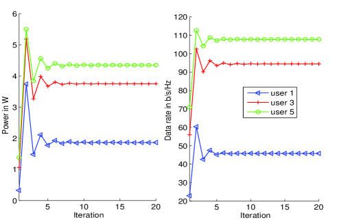
Figure 1: Data rates and power levels of users in our proposed opportunistic power control algorithm. Channel conditions for user $i+1$ is better than that of user $i$.

For the opportunistic power control, the system has 20 sub-channels. The interfering channel gain from the transmitter of user $j$ to the receiver of user $i$ on sub-channel $l$ is chosen randomly from $(0,\frac{0.1}{i})$, where $i$ denotes the user number, and the normalized noise power is set to 0.01 Watts. Accordingly, the channel conditions become better from user 1 to user 5. For an instance of the network realization, we run the proposed algorithm and show the results in Fig. 1. Note that user 1 whose sub-channels are bad consumes less power and achieves a low data rate, and user 5 with the best sub-channels transmits with high power and achieves a high data rate.

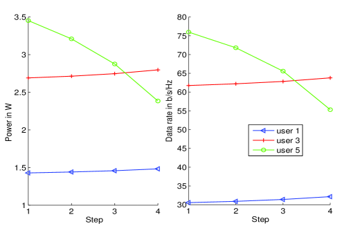
Figure 2: Data rates and power levels of users in our proposed opportunistic power control algorithm when channel conditions for user 5 gradually worsens.

Next, we fix the channel conditions of all users except user 5 for which in four steps, we gradually deteriorate its channel conditions. The results are shown in Fig. 2. As expected, user 5 decreases its transmit power levels, and as the conditions for other users improve, they increase their transmit power levels.

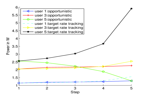
Figure 3: Comparison of power levels in our algorithm and those in (III-A) when channel conditions for user 5 gradually worsens.

As stated earlier, the behavior of the proposed algorithm is in the opposite direction of tracking a target data rate as in (III-A). We repeat our simulations and compare the results to those of (III-A) in Fig. 3. As can be seen, in (III-A), as the channel condition of user 5 deteriorates, its transmit power is increased to achieve its target data rate. This is in contrast to our proposed algorithm, where this user decreases its transmit power to reduce its interference to other users. Note that, in our proposed opportunistic scheme, at step 4, there is a 37 percent reduction in the transmit power as compared to that of the power minimization game (III-A), but the total data rate is reduced by 9 percent, which shows the efficiency of our proposed scheme. In addition, using (III-A) may cause the system to become infeasible, whereas this would not happen in our proposed game.

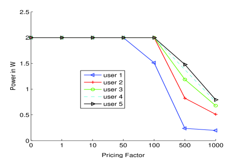
Figure 4: The effect of pricing on the converged power levels.

In the sequel, we present simulation results for the proposed pricing. The network setup is similar to the previous simulations except that now we have 10 sub-channels. First we show the effect of pricing on the users’ transmit power levels in Fig. 4. Note that pricing affects those users with bad channels more than other users, and forces such users to reduce their transmit power levels more than those users with good channels, as we desired.

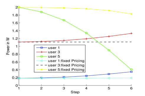
Figure 5: Comparison of converged values of power levels using fixed pricing and those of our proposed pricing when channel conditions for user 5 gradually worsens.

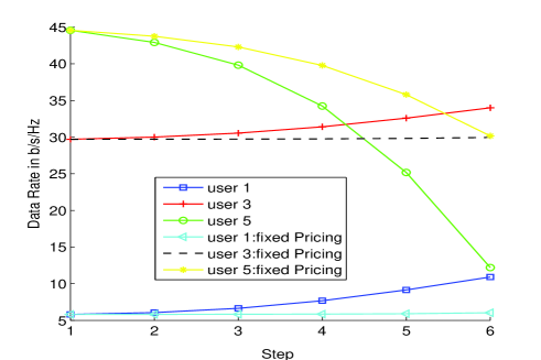
Figure 6: Comparison of converged data rates using fixed pricing and those of our proposed pricing when channel conditions for user 5 gradually worsens.

In the next two simulations, we compare the effects of our proposed pricing with those of fixed pricing used in [17]. We first run the algorithm with our proposed pricing, and after convergence, use the multiplication of pricing and the effective interference over each sub-channel as the fixed pricing in [17]. We then use the fixed pricing for subsequent steps in which the channel for user 5 gradually deteriorates. The power levels are shown in Fig. 5, and data rates in Fig. 6. Note that, at step 6 for our proposed pricing, the total data rates of users is about 3 percent less than that of the fixed pricing, but the total transmit power levels is about 15 percent less than that of the fixed pricing.

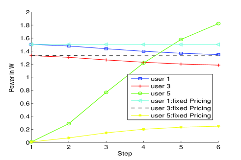
Figure 7: Comparison of converged power levels using fixed pricing and those of our proposed pricing when channel conditions for user 5 gradually improves.

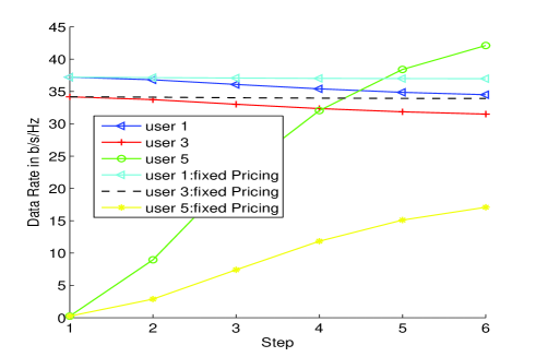
Figure 8: Comparison of converged data rates using fixed pricing and those of our proposed pricing when channel conditions for user 5 gradually improves.

Next simulations reverse the previous one, meaning that the channels for user 5 are gradually improved at successive steps. The power levels are shown in Fig. 7, and data rates in Fig. 8. Note that at step 6, the total data rates of users as well as the total transmit power levels are about 10 percent higher as compared to those of the fixed pricing.

VI Conclusions

We proposed an opportunistic power control for multi-carrier systems, in which each sub-channel is shared among all users. In such a power control framework, each user transmits at lower power levels on bad sub-channels, and does the opposite on good sub-channels. We showed that in the proposed game there always exists a generalized Nash equilibrium, and provided the sufficient conditions for GNE’s uniqueness and for convergence of the distributed algorithm. Furthermore, we proposed a pricing mechanism for the data rate maximization problem when the total transmit power of each user is constrained depending on the interference levels on sub-channels. In such cases, we also provided the sufficient conditions for GNE’s uniqueness, and for convergence of the distributed algorithm. By way of simulations, we demonstrated the improved performances of our proposed schemes as compared to those of existing algorithms.

Appendix A Proof of Theorem 3

We utilize variational inequalities to prove the uniqueness of NE for the game (III-A). To do so, we use the following definition for variational inequalities.

Definition 2 [15]: The variational inequality denoted by $VI(\mathcal{K},\textbf{F})$, where $\mathcal{K}$ is a subset of $\mathbb{R}^{n}$ and $\textbf{F}:\mathcal{K}\rightarrow\mathbb{R}^{n}$, is to find a vector $\textbf{x}\in\mathcal{K}$ such that $(\textbf{y}-\textbf{x})^{\text{T}}\textbf{F}(\textbf{x})\geq 0$ for all $\textbf{y}\in\mathcal{K}$.

For the opportunistic power control game (III-A), the strategy space of each user depends on the strategies chosen by other users. Therefore, we cannot directly apply the variational inequality formulation to the game, and some reformulations are needed. Let $\mu_{i}^{l}$ be the multiplier corresponding to the nonnegativity constraint and $\lambda_{i}$ the multiplier of the power constraint (10). The KKT conditions of the optimization problem (III-A) are

$$\hskip 85.35826pt-1+2\lambda_{i}p_{i}^{l}(I_{i}^{l})^{2}-\mu_{i}^{l}=0,~{}~{}\forall l,i,$$ (27)

$$\mu_{i}^{l}\geq 0~{}\bot~{}p_{i}^{l}\geq 0,~{}~{}\forall l,i,$$

$$\lambda_{i}\geq 0~{}\bot~{}\sum\limits_{l}({p_{i}^{l}I_{i}^{l}})^{2}\leq\varsigma_{i},~{}~{}\forall i,$$ (28)

where $\textbf{a}\bot\textbf{b}$ means that vectors a and b are perpendicular. Note that $\lambda_{i}>0$, otherwise the condition (27) will lead to $\mu_{i}^{l}<0$, which contradicts (27). This means that the constraint $\sum\limits_{l}{p_{i}^{l}I_{i}^{l}}^{2}\leq\varsigma_{i}$ is satisfied with equality. By eliminating the multipliers $\mu_{i}^{l}$, the KKT conditions can be reformulated as a nonlinear complementarity problem

$$\hskip 85.35826ptp_{i}^{l}\geq 0~{}\bot~{}-1+2\lambda_{i}p_{i}^{l}(I_{i}^{l})^{2}\geq 0,~{}~{}\forall l,i,$$ (30)

$$\lambda_{i}\geq 0~{}\bot~{}\sum\limits_{l}({p_{i}^{l}I_{i}^{l}})^{2}-\varsigma_{i}=0,~{}~{}\forall i.$$

We define the variable $q_{i}^{l}$ by

$$q_{i}^{l}=({p_{i}^{l}I_{i}^{l}})^{2},$$ (31)

and use it to reformulate (10) as

$$\sum\limits_{l}q_{i}^{l}=\varsigma_{i}.$$ (32)

Note that $q_{i}^{l}=0$ if and only if $p_{i}^{l}=0$. On the other hand, for each value of $\mathbf{q}^{l}=[q_{i}^{l}]_{i=1}^{M}$, the corresponding values of $p_{i}^{l}$ can be obtained using the OPC algorithm. Hence, we write $p_{i}^{l}=\theta_{i}^{l}(\mathbf{q}^{l})$. Since $\theta_{i}^{l}(\cdot)$ is a continuous function of $\mathbf{q}^{l}$ [6], and considering $p_{i}^{l}$ and $I_{i}^{l}$ as functions of $\mathbf{q}^{l}$, we reformulate the conditions (30) and (30) by

$$\hskip 85.35826ptq_{i}^{l}\geq 0~{}\bot~{}-1+2\lambda_{i}p_{i}^{l}(I_{i}^{l})^{2}\geq 0,~{}~{}\forall l,i,$$ (34)

$$\lambda_{i}\geq 0~{}\bot~{}\sum\limits_{l}q_{i}^{l}=\varsigma_{i},~{}~{}\forall i,.$$

Note that the variable $q_{i}^{l}$ is nonnegative, i.e., $q_{i}^{l}>0$. One can see from (16) that $p_{i}^{l}$ is always positive, i.e., $p_{i}^{l}>0$, and since $I_{i}^{l}>0$, we have $q_{i}^{l}>0$. The maximum power level for each user on each sub-channel is $\overline{p}_{i}^{l}=\frac{\sqrt{\varsigma_{i}}}{\hat{\eta}_{i}^{l}}$.

Now suppose that all users except user $i$ transmit at their maximum power levels only on sub-channel $l$. The minimum power level of user $i$ on sub-channel $l$, denoted by $\underline{p}_{i}^{l}$, is obtained from (16). Therefore, $q_{i}^{l}>\underline{q}_{i}^{l}$, where $\underline{q}_{i}^{l}=(\underline{p}_{i}^{l}\underline{I}_{i}^{l})^{2}-\sigma$ and $\sigma$ is a small positive constant, and $\underline{I}_{i}^{l}=\hat{\eta}_{i}^{l}$. From the above, we change the conditions (34) and (34) as

$$\hskip 85.35826ptq_{i}^{l}-\underline{q}_{i}^{l}\geq 0~{}\bot~{}-1+2\lambda_{i}p_{i}^{l}(I_{i}^{l})^{2}\geq 0,~{}~{}\forall l,i,$$ (36)

$$\lambda_{i}\geq 0~{}\bot~{}\sum\limits_{l}q_{i}^{l}=\varsigma_{i},~{}~{}\forall i.$$

The conditions in (36) and (36) are not equivalent to (34) and (34). However, all solutions to (34) and (34) are also solutions to (36) and (36). The change in (34) may yield additional solutions to (36) and (36). Thus, solutions to (36) and (36) consist of all solutions to (34) and (34) plus possible other solutions. Note that $\lambda_{i}>0$. We further reformulate (36) and (36) into a more suitable form as

$$\hskip 85.35826ptq_{i}^{l}-\underline{q}_{i}^{l}\geq 0~{}\bot~{}\xi_{i}-\log(p_{i}^{l})+\log(q_{i}^{l})\geq 0,~{}~{}\forall l,i,$$ (38)

$$\xi_{i}\in\mathbb{R},~{}~{}\sum\limits_{l}q_{i}^{l}=\varsigma_{i},~{}~{}\forall i.$$

We use log transform because we wish to eliminate the multiplication of the power $p_{i}^{l}$ and the effective interference $I_{i}^{l}$. It is obvious that (38) and (38) are the KKT conditions of the variational inequality $VI(\mathcal{X},\textbf{F})$ where $\mathcal{X}=\prod\limits_{i}\mathcal{X}_{i}$ and $\mathcal{X}_{i}=\{\mathbf{q}_{i}\in\mathbb{R}^{L}:q_{i}^{l}\geq\underline{q}_{i}^{l},\sum\limits_{l}q_{i}^{l}=\varsigma_{i}\}$, and $F_{i}^{l}=\log(q_{i}^{l})-\log(p_{i}^{l})$. With this modification, we now provide conditions for GNE’s uniqueness. Note that all GNEs of the game are solutions to $VI(\mathcal{X},\textbf{F})$. However, the variational inequality may have additional solutions. Hence, the conditions for uniqueness of the solution to $VI(\mathcal{X},\textbf{F})$ guarantee GNE’s uniqueness as well. This condition, however, may be excessive, since solutions to $VI(\mathcal{X},\textbf{F})$ may not be the GNE of the game.

Let $\widehat{\textbf{q}}=\mathbf{q}(1)$ and $\widetilde{\textbf{q}}=\mathbf{q}(2)$ be two solutions to $VI(\mathcal{X},\textbf{F})$. This means that for each user $i$, we have

$$\sum\limits_{l}(q_{i}^{l}(2)-q_{i}^{l}(1))\left(-\log({p}_{i}^{l}(1))+\log(q_{i}^{l}(1))\right)\geq 0,$$ (39)

$$\sum\limits_{l}(q_{i}^{l}(1)-q_{i}^{l}(2))\left(-\log({p}_{i}^{l}(2))+\log(q_{i}^{l}(2))\right)\geq 0.$$ (40)

In addition, from the definition of $q_{i}^{l}$, we have

$$\log(q_{i}^{l}(2))-\log(q_{i}^{l}(1))=2\left(\log({p}_{i}^{l}(2))-\log({p}_{i}^{l}(1))+\log({I}_{i}^{l}(2))-\log({I}_{i}^{l}(1))\right).$$ (41)

We add (39) and (40), and write

$$\sum\limits_{l}(q_{i}^{l}(1)-q_{i}^{l}(2))\left(\log({p}_{i}^{l}(2))-\log({p}_{i}^{l}(1))+2\log({I}_{i}^{l}(2))-2\log({I}_{i}^{l}(1))\right)\geq 0.$$ (42)

From the mean value theorem, we know that there exists a $q_{i}^{l}(1)\leq q_{i}^{l}\leq q_{i}^{l}(2)$ such that

$$q_{i}^{l}(1)-q_{i}^{l}(2)=q_{i}^{l}\left(\log(q_{i}^{l}(1))-\log(q_{i}^{l}(2))\right).$$ (43)

Therefore, using (41) and (43), (42) can be written as

$$\hskip 28.45274pt\sum\limits_{l}q_{i}^{l}\left(\log({p}_{i}^{l}(1))-\log({p}_{i}^{l}(2))+\log({I}_{i}^{l}(1))-\log({I}_{i}^{l}(2)\right)$$ (44)

$$\left(\log({p}_{i}^{l}(2))-\log({p}_{i}^{l}(1))+2\log({I}_{i}^{l}(2))-2\log({I}_{i}^{l}(1))\right)\geq 0.$$

Rearranging (44) and using Schwarz’s inequality, we get

$$\sqrt{\sum\limits_{l}q_{i}^{l}\left(\log({p}_{i}^{l}(1))-\log({p}_{i}^{l}(2))\right)^{2}}\leq 3\sqrt{\sum\limits_{l}q_{i}^{l}\left(\log({I}_{i}^{l}(1))-\log({I}_{i}^{l}(2))\right)^{2}},$$ (45)

or equivalently

$$\|\sqrt{\mathbf{q}}(\log({\textbf{p}}(1))-\log({\textbf{p}}(2)))\|\leq 3\|\sqrt{\mathbf{q}}(\log({\textbf{I}}(1))-\log({\textbf{I}}(2)))\|,$$ (46)

where $\|\cdot\|$ denotes the Euclidian norm. Again, we use the mean value theorem for $\log({p}_{i}^{l})$ and $\log({I}_{i}^{l})$, and write

$$\sqrt{\sum\limits_{l}q_{i}^{l}(\frac{{p}_{i}^{l}(1)-{p}_{i}^{l}(2)}{p_{i}^{l}})^{2}}\leq 3\sqrt{\sum\limits_{l}q_{i}^{l}(\frac{{I}_{i}^{l}(1)-{I}_{i}^{l}(2)}{I_{i}^{l}})^{2}},$$ (47)

and

$$\sqrt{\sum\limits_{l}q_{i}^{l}(\frac{{p}_{i}^{l}(1)-{p}_{i}^{l}(2)}{p_{i}^{l}})^{2}}\leq 3\sqrt{\sum\limits_{l}q_{i}^{l}(\frac{1}{I_{i}^{l}}\sum\limits_{j\neq i}\hat{G}_{i,j}^{l}({p}_{j}^{l}(1)-{p}_{j}^{l}(2)))^{2}}.$$ (48)

Note that $p_{i}^{l}\leq\frac{\sqrt{\varsigma_{i}}}{\hat{\eta}_{i}^{l}}$, $I_{i}^{l}\geq\hat{\eta}_{i}^{l}$, and $\underline{q}_{i}^{l}\leq q_{i}^{l}\leq\varsigma_{i}$. From (49), we obtain

$$\frac{1}{\sqrt{\varsigma_{i}}}\min_{l}(\sqrt{\underline{q}_{i}^{l}}\hat{\eta}_{i}^{l})\sqrt{\sum\limits_{l}({p}_{i}^{l}(1)-{p}_{i}^{l}(2))^{2}}\leq 3\sum\limits_{j\neq i}\sqrt{\varsigma_{i}}\max_{l}\frac{\hat{G}_{i,j}^{l}}{\hat{\eta}_{i}^{l}}\sqrt{\sum\limits_{l}({p}_{j}^{l}(1)-{p}_{j}^{l}(2))^{2}}.$$ (49)

Defining $[\textbf{a}]_{i}=\sqrt{\sum\limits_{l}(p_{i}^{l}(1)-p_{i}^{l}(2))^{2}}$ and considering the matrix A defined in (17), we obtain $\textbf{A}\textbf{a}\leq\textbf{0}$. Therefore, if the matrix A is a P-matrix, we have $\textbf{a}=\textbf{0}$, and hence the proof.

Appendix B Proof of Theorem 4

From (49), one obtains

$$\sqrt{\sum\limits_{l}({p}_{i}^{l}(1)-{p}_{i}^{l}(2))^{2}}\leq 3\sum\limits_{j\neq i}\frac{\sqrt{\varsigma_{i}}\max_{l}\frac{\hat{G}_{i,j}^{l}}{\hat{\eta}_{i}^{l}}}{\frac{1}{\sqrt{\varsigma_{i}}}\min_{l}(\sqrt{\underline{q}_{i}^{l}}\hat{\eta}_{i}^{l})}\sqrt{(\sum\limits_{l}({p}_{j}^{l}(1)-{p}_{j}^{l}(2)))^{2}},$$ (50)

If the matrix

$$[\widehat{\textbf{{B}}}]_{i,j}=\left\{\begin{array}[]{ll}~{}1&\mbox{\text{if} $i=j$},\\ -3\frac{\sqrt{\varsigma_{i}}\max_{l}\frac{\hat{G}_{i,j}^{l}}{\hat{\eta}_{i}^{l}}}{\frac{1}{\sqrt{\varsigma_{i}}}\min_{l}(\sqrt{\underline{q}_{i}^{l}}\hat{\eta}_{i}^{l})}&\mbox{\text{if} $i\neq j$},\end{array}\right.$$ (51)

is a P-matrix, GNE is unique. From the P-property of the matrix, this is equivalent to the spectral condition in (18).

Appendix C Proof of Theorem 5

Note that at each iteration, say $n+1$, the parameters $q_{i}^{l}$ and power vectors are related by

$$q_{i}^{l}(n+1)=(p_{i}^{l}(n+1)I_{i}^{l}(\textbf{p}(n))^{2}.$$ (52)

Since they are the solutions of the game (III-A), we have

$$\hskip 85.35826ptq_{i}^{l}(n+1)-\underline{q}_{i}^{l}\geq 0,~{}~{}\xi_{i}^{n+1}-\log(p_{i}^{l}(n+1))+\log(q_{i}^{l}(n+1))\geq 0,$$ (54)

$$\xi_{i}^{n+1}\in\mathbb{R},~{}~{}\sum\limits_{l}q_{i}^{l}(n+1)=\varsigma_{i}.$$

Therefore, with ${p}_{i}^{l}(1)=p_{i}^{l}(n+1)$ and ${p}_{i}^{l}(2)=p_{i}^{l*}$, where $p_{i}^{l*}$ is the GNE of the game, one can follow the same line as in proof of Theorem 3 to obtain the following inequality

$$\frac{1}{\sqrt{\varsigma_{i}}}\min_{l}(\sqrt{\underline{q}_{i}^{l}}\hat{\eta}_{i}^{l})\sqrt{\sum\limits_{l}(p_{i}^{l}(n+1)-p_{i}^{l*})^{2}}\leq 3\sum\limits_{j\neq i}\sqrt{\varsigma_{i}}\max_{l}\frac{\hat{G}_{i,j}^{l}}{\hat{\eta}_{i}^{l}}\sqrt{(\sum\limits_{l}(p_{j}^{l}(n+1)-p_{j}^{l*}))^{2}}.$$ (55)

Using (55) and the P-property of matrix A defined in (17), one can easily derive the condition.

Appendix D Proof of Theorem 7

Let $\mu_{i}$ be the multiplier corresponding to the power constraint (IV). The KKT conditions for the optimization problem (IV) can be reformulated as the following complementarity problem

$$\hskip 34.14322ptp_{i}^{l}\geq 0~{}\bot~{}-(\frac{1}{\sum\limits_{j}{{\hat{G}_{i,j}^{l}}{p_{j}^{l}}}+\hat{\eta}_{i}^{l}})+\lambda_{i}I_{i}^{l}+\mu_{i}\geq 0,~{}~{}\forall l,i,$$ (57)

$$\mu_{i}\geq 0~{}\bot~{}\sum\limits_{l}p_{i}^{l}\leq P_{i},~{}~{}\forall i.$$

These are the KKT conditions for $VI(\mathcal{X},\textbf{F})$, where $\mathcal{X}=\prod\limits_{i}\mathcal{X}_{i}$ and $\mathcal{X}_{i}=\{\textbf{p}_{i}\in\mathbb{R}^{L}:p_{i}^{l}\geq 0,\sum\limits_{l}p_{i}^{l}\leq P_{i}\}$, and

$$F_{i}^{l}(\textbf{p})=-(\frac{1}{\sum\limits_{j}{{\hat{G}_{i,j}^{l}}{p_{j}^{l}}}+\hat{\eta}_{i}^{l}})+\lambda_{i}I_{i}^{l}.$$ (58)

Since each set $\mathcal{X}_{i}$ is closed and convex, and $F_{i}^{l}(\cdot)$ is continuous, $VI(\mathcal{X},\textbf{F})$ has a solution. Since the set $\mathcal{X}$ is a Cartesian product of some independent closed and convex sets, it is known [15] that $VI(\mathcal{X},\textbf{F})$ has a unique solution if $\textbf{F}(\cdot)$ is uniformly P-function, which means that there exists a constant $c$ such that for every $\textbf{p}\in\mathcal{X}$ and $\textbf{p}^{\prime}\in\mathcal{X}$, we have

$$\max_{i}(\textbf{p}_{i}-\textbf{p}_{i}^{\prime})(\textbf{F}_{i}(\textbf{p})-\textbf{F}_{i}(\textbf{p}))\geq c\|\textbf{p}-\textbf{p}^{\prime}\|^{2}.$$ (59)

Therefore, it suffices to prove that the function $F(\cdot)$ is uniformly P-function. For $\textbf{F}(\cdot)$, we have

$$F_{i}^{l}(\textbf{p})-F_{i}^{l}(\textbf{p}^{\prime}))=\frac{\sum\limits_{j}{{\hat{G}_{i,j}^{l}}({p_{j}^{l}}-{p_{j}^{l}}^{\prime})}}{(\sum\limits_{j}{{\hat{G}_{i,j}^{l}}{{p_{j}^{l}}}}+\hat{\eta}_{i}^{l})(\sum\limits_{j}{{\hat{G}_{i,j}^{l}}{{p_{j}^{l}}}^{\prime}}+\hat{\eta}_{i}^{l})}+\lambda_{i}\sum\limits_{j\neq i}{{\hat{G}_{i,j}^{l}}({p_{j}^{l}}-{p_{j}^{l}}^{\prime})}.$$ (60)

We define the following variables

$$\psi_{i}^{l}=\sqrt{(\sum\limits_{j}{{\hat{G}_{i,j}^{l}}{{p_{j}^{l}}}}+\hat{\eta}_{i}^{l})(\sum\limits_{j}{{\hat{G}_{i,j}^{l}}{{p_{j}^{l}}}^{\prime}}+\hat{\eta}_{i}^{l})},$$ (61)

and write

$$\hskip 2.84544pt(\textbf{p}_{i}-\textbf{p}_{i}^{\prime})(\textbf{F}_{i}(\textbf{p})-\textbf{F}_{i}(\textbf{p}))=\sum\limits_{l}(p_{i}^{l}-{p_{i}^{l}}^{\prime})\frac{\sum\limits_{j}{{\hat{G}_{i,j}^{l}}({p_{j}^{l}}-{p_{j}^{l}}^{\prime})}}{(\sum\limits_{j}{{\hat{G}_{i,j}^{l}}{{p_{j}^{l}}}}+\hat{\eta}_{i}^{l})(\sum\limits_{j}{{\hat{G}_{i,j}^{l}}{{p_{j}^{l}}}^{\prime}}+\hat{\eta}_{i}^{l})}$$ (65)

$$+\lambda_{i}\sum\limits_{j\neq i}{{\hat{G}_{i,j}^{l}}({p_{j}^{l}}-{p_{j}^{l}}^{\prime})}=\sum\limits_{l}\frac{(p_{i}^{l}-{p_{i}^{l}}^{\prime})^{2}}{{\psi_{i}^{l}}^{2}}+\sum\limits_{l}\frac{(p_{i}^{l}-{p_{i}^{l}}^{\prime})\sum\limits_{j\neq i}{{\hat{G}_{i,j}^{l}}\left(1+\lambda_{i}{\psi_{i}^{l}}^{2}\right)({p_{j}^{l}}-{p_{j}^{l}}^{\prime})}}{{\psi_{i}^{l}}^{2}}$$

$$\geq\sum\limits_{l}\frac{(p_{i}^{l}-{p_{i}^{l}}^{\prime})^{2}}{{\psi_{i}^{l}}^{2}}-\sum\limits_{j\neq i}\left|\sum\limits_{l}(p_{i}^{l}-{p_{i}^{l}}^{\prime})(p_{j}^{l}-{p_{j}^{l}}^{\prime})\frac{{\hat{G}_{i,j}^{l}}\left(1+\lambda_{i}{\psi_{i}^{l}}^{2}\right)}{{\psi_{i}^{l}}^{2}}\right|$$

$$\geq\sum\limits_{l}\frac{(p_{i}^{l}-{p_{i}^{l}}^{\prime})^{2}}{{\psi_{i}^{l}}^{2}}-\sum\limits_{j\neq i}\left(\max_{l}\left(\frac{{\hat{G}_{i,j}^{l}}\left(1+\lambda_{i}{\psi_{i}^{l}}^{2}\right){\psi_{j}^{l}}}{{\psi_{i}^{l}}}\right)\sqrt{\sum\limits_{l}\frac{(p_{i}^{l}-{p_{i}^{l}}^{\prime})^{2}}{{\psi_{i}^{l}}^{2}}}\sqrt{\sum\limits_{l}\frac{(p_{j}^{l}-{p_{j}^{l}}^{\prime})^{2}}{{\psi_{j}^{l}}^{2}}}\right),$$

where we applied Schwartz’ inequality to (65). By some manipulations, one can obtain the following inequality

$$(\textbf{p}_{i}-\textbf{p}_{i}^{\prime})(\textbf{F}_{i}(\textbf{p})-\textbf{F}_{i}(\textbf{p}))\geq[\textbf{d}]_{i}[\textbf{D}\textbf{d}]_{i},$$ (66)

where d is a vector whose $i^{\text{th}}$ element is $[\textbf{d}]_{i}=\sqrt{\sum\limits_{l}\frac{(p_{i}^{l}-{p_{i}^{l}}^{\prime})^{2}}{{\psi_{i}^{l}}^{2}}}$ and D is defined in (25). From (66) and the P-property assumption on matrix D, one can show that $\textbf{F}(\cdot)$ is uniformly P-function [10, 17].

Appendix E Proof of Theorem 8

To prove the convergence of the algorithm, we follow the same line as in the proof of Theorem 5. Given the power profile $\textbf{p}(n)$ at iteration $n$, users update their power levels according to (24). This means that their power levels $p_{i}^{l}(n+1)$ must satisfy the following optimality condition

$$\sum\limits_{l}(p_{i}^{l}-p_{i}^{l}(n+1))(-\frac{1}{\sum\limits_{j\neq i}{{\hat{G}_{i,j}^{l}}{{p_{j}^{l}(n)}}}+\hat{\eta}_{i}^{l}}+\lambda I_{i}^{l}(p(n))).$$ (67)

The NE must also satisfy a similar condition, i.e.,

$$\sum\limits_{l}(p_{i}^{l}-{p_{i}^{l}}^{*})(-\frac{1}{\sum\limits_{j\neq i}{{\hat{G}_{i,j}^{l}}{{p_{j}^{l}}^{*}}}+\hat{\eta}_{i}^{l}}+\lambda I_{i}^{l}(p^{*})).$$ (68)

Adding these two inequalities and following the same steps as in Theorem 5, this theorem is proved.

References

- [1] D. Fudenberg and J. Tirole, Game Theory. Cambridge, MA: MIT Press, 1991.
- [2] Z. Han, Z. Ji, and K. J. R. Liu, “Non-cooperative resource competition game by virtual referee in multi-cell OFDMA networks,” IEEE Journal on Selected Areas in Communications, vol. 25, no. 6, pp. 1 –10, August 2007.
- [3] J.-S. Pang, G. Scutari, F. Facchinei, and C. Wang, “Distributed power allocation with rate constraints in Gaussian parallel interference channels,” IEEE Transactions on Information Theory, vol. 54, no. 8, pp. 2868 –2878, August 2008.
- [4] F. Facchinei and C. Kanzow, “Generalized Nash equilibrium problems,” 4OR, vol. 5, pp. 173– 210, 1993.
- [5] G. J. Foschini and Z. Miljanic, “A simple distributed autonomous power control algorithm and its convergence,” IEEE Transactions on Vehicular Technology, vol. 42, no. 4, pp. 641–646, November 1993.
- [6] K. Leung and C. W. Sung, “An opportunistic power control algorithm for cellular network,” IEEE/ACM Transactions on Networking, vol. 14, no. 3, pp. 470 –478, June 2006.
- [7] G. Scutari, D. P. Palomar, and S. Barbarossa, “Optimal linear precoding strategies for wideband noncooperative systems based on game theory - Part I: Nash equilibria,” IEEE Transactions on Signal Processing, vol. 56, no. 3, pp. 1230– 1249, March 2008.
- [8] ——, “Optimal linear precoding strategies for wideband noncooperative systems based on game theory Part II: Algorithms,” IEEE Transactions on Signal Processing, vol. 56, no. 3, pp. 1250 –1267, March 2008.
- [9] ——, “Asynchronous iterative water-filling for Gaussian frequency-selective interference channels,” IEEE Transactions on Information Theory, vol. 54, no. 7, pp. 2868 –2878, July 2008.
- [10] R. W. Cottle, J.-S. Pang, and R. E. Stone, The Linear Complementarity Problem. Cambridge Academic Press, 1992.
- [11] K. W. Shum, K.-K. Leung, and C. W. Sung, “Convergence of iterative waterfilling algorithm for Gaussian interference channels,” IEEE Journal on Selected Areas in Communications, vol. 25, no. 6, pp. 1091– 1100, August 2007.
- [12] D. P. Bertsekas and J. N. Tsitsiklis, Parallel and Distributed Computation: Numerical Methods, 2nd ed. Athena Scientific, 1989.
- [13] S. Boyd and L. Vandenberghe, Convex Optimization. Cambridge University Press, 2004.
- [14] Z.-Q. Luo and J.-S. Pang, “Analysis of iterative waterfilling algorithm for multiuser power control in digital subscriber lines,” EURASIP Journal on Applied Signal Processing, vol. 2006, pp. 1 –10, May 2006.
- [15] F. Facchinei and J.-S. Pang, Finite-Dimensional Variational Inequalities and Complementarity Problem. Springer-Verlag, New York, 2003.
- [16] F. Wang, M. Krunz, and S. Cui, “Price-based spectrum management in cognitive radio networks,” IEEE Journal on Selected Topics in Signal Processing, vol. 2, no. 1, p. 74 87, February 2008.
- [17] J.-S. Pang, G. Scutari, D. P. Palomar, and F. Facchinei, “Design of cognitive radio systems under temperature-interference constraints: A variational inequality approach,” IEEE Transactions on Signal Processing, vol. 58, no. 6, pp. 3251–3271, June 2010.