A General Framework for Structured Sparsity via Proximal Optimization

Abstract

We study a generalized framework for structured sparsity. It extends the well-known methods of Lasso and Group Lasso by incorporating additional constraints on the variables as part of a convex optimization problem. This framework provides a straightforward way of favouring prescribed sparsity patterns, such as orderings, contiguous regions and overlapping groups, among others. Existing optimization methods are limited to specific constraint sets and tend to not scale well with sample size and dimensionality. We propose a novel first order proximal method, which builds upon results on fixed points and successive approximations. The algorithm can be applied to a general class of conic and norm constraints sets and relies on a proximity operator subproblem which can be computed explicitly. Experiments on different regression problems demonstrate the efficiency of the optimization algorithm and its scalability with the size of the problem. They also demonstrate state of the art statistical performance, which improves over Lasso and StructOMP.

1 Introduction

We study the problem of learning a sparse linear regression model. The goal is to estimate a parameter vector $\beta^{*}\in{\mathbb{R}}^{n}$ from a vector of measurements $y\in{\mathbb{R}}^{m}$, obtained from the model $y=X\beta^{*}+\xi$, where $X$ is an $m\times n$ matrix, which may be fixed or randomly chosen, and $\xi\in{\mathbb{R}}^{m}$ is a vector resulting from the presence of noise. We are interested in sparse estimation under additional conditions on the sparsity pattern of $\beta^{*}$. In other words, not only we do expect that $\beta^{*}$ is sparse but also that it exhibits structured sparsity, namely certain configurations of its nonzero components are preferred to others. This problem arises in several applications, such as regression, image denoising, background subtraction etc. – see [11, 9] for a discussion.

In this paper, we build upon the structured sparsity framework recently proposed by [12]. It is a regularization method, formulated as a convex, nonsmooth optimization problem over a vector of auxiliary parameters. This approach provides a constructive way to favour certain sparsity patterns of the regression vector $\beta$. Specifically, this formulation involves a penalty function given by the formula $\Omega(\beta|\Lambda)=\inf\left\{\frac{1}{2}\sum_{i=1}^{n}\left(\frac{\beta_{i}^{2}}{\lambda_{i}}+\lambda_{i}\right):\lambda\in{\Lambda}\right\}$. This function can be interpreted as an extension of a well-known variational form for the $\ell_{1}$ norm. The convex constraint set ${\Lambda}$ provides a means to incorporate prior knowledge on the magnitude of the components of the regression vector. As we explain in Section 2, the sparsity pattern of $\beta$ is contained in that of the auxiliary vector ${\lambda}$ at the optimum. Hence, if the set ${\Lambda}$ allows only for certain sparsity patterns of $\lambda$, the same property will be “transferred” to the regression vector $\beta$.

In this paper, we propose a tractable class of regularizers of the above form which extends the examples described in [12]. Specifically, we study in detail the cases in which the set $\Lambda$ is defined by norm or conic constraints, combined with a linear map. As we shall see, these cases include formulations which can be used for learning graph sparsity and hierarchical sparsity, in the terminology of [9]. That is, the sparsity pattern of the vector $\beta^{*}$ may consist of a few contiguous regions in one or more dimensions, or may be embedded in a tree structure. These sparsity problems arise in several applications, ranging from functional magnetic resonance imaging [7, 22], to scene recognition in vision [8], to multi-task learning [1, 17] and to bioinformatics [19] – to mention but a few.

A main limitation of the technique described in [12] is that in many cases of interest the penalty function cannot be easily computed. This makes it difficult to solve the associated regularization problem. For example [12] proposes to use block coordinate descent, and this method is feasible only for a limited choice of the set $\Lambda$. The main contribution of this paper is an efficient proximal point method to solve regularized least squares with the penalty function $\Omega(\beta|\Lambda)$ in the general case of set $\Lambda$ described above. The method combines a fast fixed point iterative scheme, which is inspired by recent work by [13] with an accelerated first order method equivalent to FISTA [4]. We present a numerical study of the efficiency of the proposed method and a statistical comparison of the proposed penalty functions with the greedy method of [9] and the Lasso.

Recently, there has been significant research interest on structured sparsity and the literature on this subject is growing fast, see for example [1, 9, 10, 11, 23] and references therein for an indicative list of papers. In this work, we mainly focus on convex penalty methods and compare them to greedy methods [3, 9]. The latter provide a natural extension of techniques proposed in the signal processing community and, as argued in [9], allow for a significant performance improvement over more generic sparsity models such as the Lasso or the Group Lasso [23]. The former methods have until recently focused mainly on extending the Group Lasso, by considering the possibility that the groups overlap according to certain hierarchical structures [11, 24]. Very recently, general choices of convex penalty functions have been proposed [2, 12]. In this paper we build upon [12], providing both new instances of the penalty function and improved optimization algorithms.

The paper is organized as follows. In Section 2, we set our notation, review the method of [12] and present the new sets for inducing structured sparsity. In Section 3, we present our technique for computing the proximity operator of the penalty function and the resulting accelerated proximal method. In Section 4, we report numerical experiments with this method.

2 Framework and extensions

In this section, we introduce our notation, review the learning method which we extend in this paper and present the new sets for inducing structured sparsity.

We let ${\mathbb{R}}_{+}$ and ${\mathbb{R}}_{++}$ be the nonnegative and positive real line, respectively. For every $\beta\in{\mathbb{R}}^{n}$ we define $|\beta|\in{\mathbb{R}}_{+}^{n}$ to be the vector $|\beta|=(|\beta_{i}|)_{i=1}^{n}$. For every $p\geq 1$, we define the $\ell_{p}$ norm of $\beta$ as $\|\beta\|_{p}=\left(\sum_{i=1}^{n}|\beta_{i}|^{p}\right)^{\frac{1}{p}}$. If $C\subseteq{\mathbb{R}}^{n}$, we denote by $\delta_{C}:{\mathbb{R}}^{n}\rightarrow{\mathbb{R}}$ the indicator function of the set $C$, that is, $\delta_{C}(x)=0$ if $x\in C$ and $\delta_{C}(x)=+\infty$ otherwise.

We now review the structured sparsity approach of [12]. Given an $m\times n$ input data matrix $X$ and an output vector $y\in{\mathbb{R}}^{m}$, obtained from the linear regression model $y=X\beta^{*}+\xi$ discussed earlier, they consider the optimization problem

$$\inf\left\{\frac{1}{2}\|X\beta-y\|^{2}_{2}+\rho\,\Gamma(\beta,{\lambda}):\beta\in{\mathbb{R}}^{n},\lambda\in{\Lambda}\right\}$$ (2.1)

where $\rho$ is a positive parameter, ${\Lambda}$ is a prescribed convex subset of the positive orthant ${\mathbb{R}}^{n}_{++}$ and the function $\Gamma:{\mathbb{R}}^{n}\times{\mathbb{R}}_{++}^{n}\rightarrow{\mathbb{R}}$ is given by the formula

$$\Gamma(\beta,{\lambda})=\frac{1}{2}\sum_{i=1}^{n}\left(\frac{\beta_{i}^{2}}{\lambda_{i}}+\lambda_{i}\right).$$

Note that the infimum over $\lambda$ in general is not attained, however the infimum over $\beta$ is always attained. Since the auxiliary vector ${\lambda}$ appears only in the second term and our goal is to estimate $\beta^{*}$, we may also directly consider the regularization problem

$$\min\left\{\frac{1}{2}\|X\beta-y\|^{2}_{2}+\rho\,\Omega(\beta|\Lambda):\beta\in{\mathbb{R}}^{n}\right\},$$ (2.2)

where the penalty function takes the form $\Omega(\beta|\Lambda)=\inf\left\{\Gamma(\beta,{\lambda}):{\lambda}\in{\Lambda}\right\}$. This problem is still convex because the function $\Gamma$ is jointly convex [5]. Also, note that the function $\Omega$ is independent of the signs of the components of $\beta$.

In order to gain some insight about the above methodology, we note that, for every ${\lambda}\in{\mathbb{R}}_{++}^{n}$, the quadratic function $\Gamma(\cdot,{\lambda})$ provides an upper bound to the $\ell_{1}$ norm, namely it holds that $\Omega(\beta|\Lambda)\geq\|\beta\|_{1}$ and the inequality is tight if and only if $|\beta|\in{\Lambda}$. This fact is an immediate consequence of the arithmetic-geometric inequality. In particular, we see that if we choose ${\Lambda}={\mathbb{R}}_{++}^{n}$, the method (2.2) reduces to the Lasso. The above observation suggests a heuristic interpretation of the method (2.2): among all vectors $\beta$ which have a fixed value of the $\ell_{1}$ norm, the penalty function $\Omega$ will encourage those for which $|\beta|\in{\Lambda}$. Moreover, when $|\beta|\in{\Lambda}$ the function $\Omega$ reduces to the $\ell_{1}$ norm and, so, the solution of problem $\eqref{eq:method}$ is expected to be sparse. The penalty function therefore will encourage certain desired sparsity patterns.

The last point can be better understood by looking at problem (2.1). For every solution $({\hat{\beta}},{\hat{\lambda}})$, the sparsity pattern of ${\hat{\beta}}$ is contained in the sparsity pattern of ${\hat{\lambda}}$, that is, the indices associated with nonzero components of ${\hat{\beta}}$ are a subset of those of ${\hat{\lambda}}$. Indeed, if ${\hat{\lambda}}_{i}=0$ it must hold that ${\hat{\beta}}_{i}=0$ as well, since the objective would diverge otherwise (because of the ratio $\beta_{i}^{2}/\lambda_{i}$). Therefore, if the set ${\Lambda}$ favours certain sparse solutions of ${\hat{\lambda}}$, the same sparsity pattern will be reflected on ${\hat{\beta}}$. Moreover, the regularization term $\sum_{i}\lambda_{i}$ favours sparse vectors $\lambda$. For example, a constraint of the form ${\lambda}_{1}\geq\dots\geq{\lambda}_{n}$, favours consecutive zeros at the end of $\lambda$ and nonzeros everywhere else. This will lead to zeros at the end of $\beta$ as well. Thus, in many cases like this, it is easy to incorporate a convex constraint on $\lambda$, whereas it may not be possible to do the same with $\beta$.

In this paper we consider sets $\Lambda$ of the form

$$\Lambda=\{\lambda\in{\mathbb{R}}^{n}_{++}:A{\lambda}\in S\}$$

where $S$ is a convex set and $A$ is a $k\times n$ matrix. Two main choices of interest are when $S$ is a convex cone or the unit ball of a norm. We shall refer to the corresponding set $\Lambda$ as conic constraint or norm constraint set, respectively. We next discuss two specific examples, which highlight the flexibility of our approach and help us understand the sparsity patterns favoured by each choice.

Within the conic constraint sets, we may choose $S={\mathbb{R}}_{++}^{k}$, so that ${\Lambda}=\{{\lambda}\in{\mathbb{R}}^{n}_{++}:A{\lambda}\geq 0\}$, which can be used to encourage hierarchical sparsity. In [12] they considered the set $\Lambda=\{\lambda\in{\mathbb{R}}^{n}_{++}:\lambda_{1}\geq\dots\geq\lambda_{n}\}$ and derived an explicit formula of the corresponding regularizer $\Omega(\beta|\Lambda)$. Note that for a generic matrix $A$ the penalty function cannot be computed explicitly. In Section 3, we show how to overcome this difficulty.

Within the norm constraint sets, we may choose $S$ to be the $\ell_{1}$-unit ball and $A$ the edge map of a graph $G$ with edge set $E$, so that ${\Lambda}=\left\{{\lambda}\in{\mathbb{R}}^{n}_{++}:\sum_{(i,j)\in E}|\lambda_{i}-\lambda_{j}|\leq 1\right\}.$ This set can be used to encourage sparsity patterns consisting of few connected regions/subgraphs of the graph $G$. For example if $G$ is a 1D-grid we have that ${\Lambda}=\{{\lambda}\in{\mathbb{R}}^{n}_{++}:\sum_{i=1}^{n-1}|\lambda_{i+1}-\lambda_{i}|\leq 1\}$, so the corresponding penalty will favour vectors $\beta$ whose absolute values are constant.

For a generic convex set ${\Lambda}$, since the penalty function $\Omega$ is not easily computable, one needs to deal directly with problem (2.1). To this end, we recall here the definition of the proximity operator [14].

Definition 2.1.

Let ${\varphi}$ be a real-valued convex function on ${\mathbb{R}}^{d}$. The proximity operator of ${\varphi}$ is defined, for every $t\in{\mathbb{R}}^{d}$ by $\operatorname{prox}_{\varphi}(t):=\operatorname{argmin}\left\{\dfrac{1}{2}\|z-t\|_{2}^{2}+{\varphi}(z):z\in{\mathbb{R}}^{d}\right\}$.

The proximity operator is well-defined, because the above minimum exists and is unique.

3 Optimization Method

In this section, we discuss how to solve problem (2.1) using an accelerated first-order method that scales linearly with respect to the problem size, as we later show in the experiments. This method relies on the computation of the proximity operator of the function $\Gamma$, restricted to ${\mathbb{R}}^{n}\times\Lambda$. Since the exact computation of the proximity operator is possible only in simple special cases of sets $\Lambda$, we present here an efficient fixed-point algorithm for computing the proximity operator that can be applied to a wide variety of constraints. Finally, we discuss an accelerated proximal method that uses our algorithm.

3.1 Computation of the Proximity Operator

According to Definition 2.1, the proximal operator of $\Gamma$ at $(\alpha,\mu)\in{\mathbb{R}}^{n}\times{\mathbb{R}}^{n}$ is the solution of the problem

$$\min\left\{\frac{1}{2}\|(\beta,{\lambda})-(\alpha,\mu)\|^{2}_{2}+\rho\,\Gamma(\beta,{\lambda}):\beta\in{\mathbb{R}}^{n},{\lambda}\in\Lambda\right\}.$$ (3.1)

For fixed ${\lambda}$, a direct computation yields that the objective function in (3.1) attains its minimum at

$$\beta_{i}({\lambda})=\frac{\alpha_{i}{\lambda}_{i}}{{\lambda}_{i}+\rho}.$$ (3.2)

Using this equation we obtain the simplified problem

$$\min\left\{\frac{1}{2}\|{\lambda}-\mu\|^{2}+\frac{\rho}{2}\sum_{i=1}^{n}\left(\frac{\alpha_{i}^{2}}{{\lambda}_{i}+\rho}+{\lambda}_{i}\right):\lambda\in\Lambda\right\}.$$ (3.3)

This problem can still be interpreted as a proximity map computation. We discuss how to solve it under our general assumption ${\Lambda}=\{{\lambda}\in{\mathbb{R}}^{n}_{++}:A{\lambda}\in S\}$. Moreover, we assume that the projection on the set $S$ can be easily computed. To this end, we define the $(n+k)\times n$ matrix $B^{\scriptscriptstyle\top}=[I,A^{\scriptscriptstyle\top}]$ and the function ${\varphi}(s,t)={\varphi}_{1}(s)+{\varphi}_{2}(t)$, $(s,t)\in{\mathbb{R}}^{n}\times{\mathbb{R}}^{k}$, where

$${\varphi}_{1}(s)=\frac{\rho}{2}\sum_{i=1}^{n}\left(\frac{\alpha_{i}^{2}}{s_{i}+\rho}+s_{i}+\delta_{{\mathbb{R}}_{++}}(s_{i})\right),$$

and ${\varphi}_{2}(t)=\delta_{S}(t)$. Note that the solution of problem (3.3) is the same as the proximity map of the linearly composite function ${\varphi}\circ B$ at $\mu$, which solves the problem

$$\min\left\{\frac{1}{2}\|{\lambda}-\mu\|^{2}+{\varphi}(B\lambda):\lambda\in{\mathbb{R}}^{n}\right\}.$$

At first sight this problem seems difficult to solve. However, it turns out that if the proximity map of the function ${\varphi}$ has a simple form, the following theorem adapted from [13, Theorem 3.1] can be used to accomplish this task. For ease of notation we set $d=n+k$.

Theorem 3.1.

Let ${\varphi}$ be a convex function on ${\mathbb{R}}^{d}$, $B$ a $d\times n$ matrix, $\mu\in{\mathbb{R}}^{n}$, $c>0$, and define the mapping $H:{\mathbb{R}}^{d}\rightarrow{\mathbb{R}}^{d}$ at $v\in{\mathbb{R}}^{d}$ as

$$H(v)=(I-\operatorname{prox}_{\frac{{\varphi}}{c}})((I-cBB^{\scriptscriptstyle\top})v+B\mu).$$

Then, for any fixed point ${\hat{v}}$ of $H$, it holds that

$$\operatorname{prox}_{{\varphi}\circ B}(\mu)=\mu-cB^{\scriptscriptstyle\top}{\hat{v}}.$$ (3.4)

The Picard iterates $\{v_{s}:s\in{\mathbb{N}}\}\subseteq{\mathbb{R}}^{d}$, starting at $v_{0}\in{\mathbb{R}}^{d}$, are defined by the recursive equation $v_{s}=H(v_{s-1})$. Since the operator $I-\operatorname{prox}_{{\varphi}}$ is nonexpansive (see e.g. [6]), the map $H$ is nonexpansive if $c\in\left[0,\frac{2}{||B||^{2}}\right]$. Despite this, the Picard iterates are not guaranteed to converge to a fixed point of $H$. However, a simple modification with an averaging scheme can be used to compute the fixed point.

Theorem 3.2.

[18] Let $H:{\mathbb{R}}^{d}\rightarrow{\mathbb{R}}^{d}$ be a nonexpansive mapping which has at least one fixed point and let $H_{{\kappa}}:={{\kappa}}I+(1-{{\kappa}})H$. Then, for every ${{\kappa}}\in(0,1)$, the Picard iterates of $H_{{\kappa}}$ converge to a fixed point of $H$.

The required proximity operator of ${\varphi}$ is directly given, for every $(s,t)\in{\mathbb{R}}^{n}\times{\mathbb{R}}^{k}$, by

$$\operatorname{prox}_{\varphi}(s,t)=\left(\operatorname{prox}_{{\varphi}_{1}}(s),\operatorname{prox}_{{\varphi}_{2}}(t)\right).$$

Both $\operatorname{prox}_{{\varphi}_{1}}$ and $\operatorname{prox}_{{\varphi}_{2}}$ can be easily computed. The latter requires computing the projection on the set $S$. The former requires, for each component of the vector $s\in{\mathbb{R}}^{n}$, the solution of a cubic equation as stated in the next lemma.

Lemma 3.1.

For every $\mu,\alpha\in{\mathbb{R}}$ and $r,\rho>0$, the function $h:{\mathbb{R}}_{+}\rightarrow{\mathbb{R}}$ defined at $s$ as $h(s):=(s-\mu)^{2}+r\left(\frac{\alpha^{2}}{s+\rho}+s\right)$ has a unique minimum on its domain, which is attained at $(x_{0}-\rho)_{+}$, where $x_{0}$ is the largest real root of the polynomial $2x^{3}+(r-2(\mu+\rho))x^{2}-r\alpha^{2}$.

Proof.

Setting the derivative of $h$ equal to zero and making the change of variable $x=s+\rho$ yields the polynomial stated in the lemma. Let $x_{0}$ be the largest root of this polynomial. Since the function $h$ is strictly convex on its domain and grows at infinity, its minimum can be attained only at one point, which is $x_{0}-\rho$, if $x_{0}>\rho$, and zero otherwise. ∎

3.2 Accelerated Proximal Method

Theorem 3.4 motivates a proximal numerical approach to solving problem (2.1) and, in turn, problem (2.2). Let $E(\beta)=\frac{1}{2}\|X\beta-y\|^{2}_{2}$ and assume an upper bound $L$ of $\|X^{\scriptscriptstyle\top}X\|$ is known. Proximal first-order methods – see [6, 4, 16, 21] and references therein – can be used for nonsmooth optimization, where the objective consists of a strongly smooth term, plus a nonsmooth part, in our case $E$ and $\Gamma+\delta_{\Lambda}$, respectively. The idea is to replace $E$ with its linear approximation around a point $w_{t}$ specific to iteration $t$. This leads to the computation of a proximity operator, and specifically in our case to $u_{t}:=(\beta_{t},\lambda_{t})\leftarrow\operatorname{argmin}\bigl{\{}\frac{L}{2}\|(\beta,{\lambda})-(w_{t}-\frac{1}{L}\nabla E(w_{t}))\|^{2}_{2}+\rho\,\Gamma(\beta,{\lambda}):\beta\in{\mathbb{R}}^{n},{\lambda}\in\Lambda\bigr{\}}$. Subsequently, the point $w_{t}$ is updated, based on the current and previous estimates of the solution $u_{t},u_{t-1},\dots$ and the process repeats.

The simplest update rule is $w_{t}=u_{t}$. By contrast, accelerated proximal methods proposed by [16] use a carefully chosen $w$ update with two levels of memory, $u_{t},u_{t-1}$. If the proximity map can be exactly computed, such schemes exhibit a fast quadratic decay in terms of the iteration count, that is, the distance of the objective from the minimal value is $O\left(\frac{1}{T^{2}}\right)$ after $T$ iterations. However, it is not known whether accelerated methods which compute the proximity operator numerically can achieve this rate. The main advantages of accelerated methods are their low cost per iteration and their scalability to large problem sizes. Moreover, in applications where a thresholding operation is involved – as in Lemma 3.1 – the zeros in the solution are exact.

Algorithm 1 NEsterov PIcard-Opial algorithm (NEPIO)

  $u_{1},w_{1}\leftarrow$ arbitrary feasible values

  for t=1,2,… do

     Compute a fixed point ${\hat{v}^{(t)}}$ of $H_{t}$ by Picard-Opial

     $u_{t+1}\leftarrow w_{t}-\frac{1}{L}\nabla E(w_{t})-\frac{c}{L}B^{\scriptscriptstyle\top}{\hat{v}^{(t)}}$

     $w_{t+1}\leftarrow\pi_{t+1}u_{t+1}-(\pi_{t+1}-1)u_{t}$

  end for

For our purposes, we use a version of accelerated methods influenced by [21] (described in Algorithm 1 and called NEPIO). According to Nesterov [16], the optimal update is $w_{t+1}\leftarrow u_{t+1}+\theta_{t+1}\left(\frac{1}{\theta_{t}}-1\right)(u_{t+1}-u_{t})$ where the sequence $\theta_{t}$ is defined by $\theta_{1}=1$ and the recursion

$$\frac{1-\theta_{t+1}}{\theta_{t+1}^{2}}=\frac{1}{\theta_{t}^{2}}\,.$$ (3.5)

We have adapted [21, Algorithm 2] (equivalent to FISTA [4]) by computing the proximity operator of $\frac{{\varphi}}{L}\circ B$ using the Picard-Opial process described in Section 3.1. We rephrased the algorithm using the sequence $\pi_{t}:=1-\theta_{t}+\sqrt{1-\theta_{t}}=1-\theta_{t}+\frac{\theta_{t}}{\theta_{t-1}}$ for numerical stability. At each iteration, the map $H_{t}$ is defined by

$$H_{t}(v):=\left(I-\operatorname{prox}_{\frac{\phi}{c}}\right)\Bigg{(}\left(I-\frac{c}{L}BB^{\scriptscriptstyle\top}\right)v-\frac{1}{L}B\Big{(}\nabla E(w_{t})-Lw_{t}\Big{)}\Bigg{)}\,.$$

We also apply an Opial averaging so that the update at stage $s$ of the proximity computation is $v_{s+1}=\kappa v_{s}+(1-\kappa)H_{t}(v_{s})$. By Theorem 3.4, the fixed point process combined with the assignment of $u$ are equivalent to $u_{t+1}\leftarrow\operatorname{prox}_{\frac{{\varphi}}{L}\circ B}\left(w_{t}-\frac{1}{L}\nabla E(w_{t})\right)$.

The reason for resorting to Picard-Opial is that exact computation of the proximity operator (3.3) is possible only in simple special cases for the set $\Lambda$. By contrast, our approach can be applied to a wide variety of constraints. Moreover, we are not aware of another proximal method for solving problems (2.1) or (2.2) and alternatives like interior point methods do not scale well with problem size. In the next section, we will demonstrate empirically the scalability of Algorithm 1, as well as the efficiency of both the proximity map computation and the overall method.

4 Numerical Simulations

In this section, we present experiments with method (2.1). The goal of the experiments is to both study the computational and the statistical estimation properties of this method. One important aim of the experiments is to demonstrate that the method is statistically competitive or superior to state-of-the-art methods while being computationally efficient. The methods employed are the Lasso, StructOMP [9] and method (2.1) with the following choices for the constraint set $\Lambda$: Grid-C, ${\Lambda}_{\alpha}=\{{\lambda}:\|A{\lambda}\|_{1}\leq\alpha\}$, where $A$ is the edge map of a 1D or 2D grid and $\alpha>0$, and Tree-C, ${\Lambda}=\{{\lambda}:A{\lambda}\geq 0\}$, where $A$ is the edge map of a tree graph.

We solved the optimization problem (2.1) either with the toolbox CVX or with the proximal method presented in Section 3. When using the proximal method, we chose the parameter from Opial’s Theorem $\kappa=0.2$ and we stopped the iterations when the relative decrease in the objective value is less than $10^{-8}$. For the computation of the proximity operator, we stopped the iterations of the Picard-Opial method when the relative difference between two consecutive iterates is smaller than $10^{-2}$. We studied the effect of varying this tolerance in the next experiments. We used the square loss and computed the Lipschitz constant $L$ using singular value decomposition.

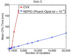
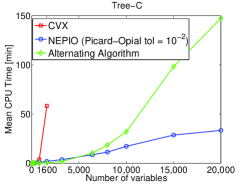
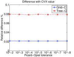
Figure 1: (Left and Centre) Computation time vs problem size for Grid-C and Tree-C. (Right) Difference with the solution obtained via CVX vs Picard-Opial tolerance.

4.1 Efficiency experiments

First, we investigated the computational properties of the proximal method. Our aim in these experiments was to show that our algorithm has a time complexity that scales linearly with the number of variables, while the sparsity and relative number of training examples is kept constant. We considered both the Grid and the Tree constraints and compared our algorithm to the toolbox CVX, which is an interior-point method solver. As is commonly known, interior-point methods are very fast, but do not scale well with the problem size. In the case of the Tree constraint, we also compared with a modified version of the alternating algorithm of [12]. For each problem size, we repeated the experiments $10$ times and we report the average computation time in Figure 1-(Left and Centre) for Grid-C and Tree-C, respectively. This result indicates that our method is suitable for large scale experiments.

We also studied the importance of the Picard-Opial tolerance for converging to a good solution. In Figure 1-Right, we report the average relative distance to the solution obtained via CVX for different values of the Picard-Opial tolerance. We considered a problem with $100$ variables and repeated the experiment $10$ times with different sampling of training examples, considering both the Grid and the Tree constraint. It is clear that decreasing the tolerance did not bring any advantage in terms of converging to a better solution, while it remarkably increased the computational overhead, passing from an average of $5s$ for a tolerance of $10^{-2}$ to $40s$ for $10^{-8}$ in the case of the Grid constraint.

Finally, we considered the 2D Grid-C case and observed that the number of Picard-Opial iterations needed to reach a tolerance of $10^{-2}$, scales well with the number of variables $n$. For example when $n$ varies between $200$ and $6400$, the average number of iterations varied between $20$ and $40$.

4.2 Statistical experiments

One dimensional contiguous regions. In this experiment, we chose a model vector $\beta^{\ast}\in{\mathbb{R}}^{200}$ with $20$ nonzero elements, whose values are random $\pm 1$. We considered sparsity patterns forming one, two, three or four non-overlapping contiguous regions, which have lengths of $20$, $10$, $7$ or $5$, respectively. We generated a noiseless output from a matrix $X$ whose elements have a standard Gaussian distribution. The estimates $\hat{\beta}$ for several models are then compared with the original. Figure 2 shows the model error $\frac{\lVert\ \hat{\beta}-\beta^{\ast}\lVert_{2}}{\lVert\ \beta^{\ast}\lVert_{2}}$ as the sample size changes from $22$ (barely above the sparsity) up to $100$ (half the dimensionality). This is the average over $50$ runs, each with a different $\beta^{\ast}$ and $X$. We observe that Grid-C outperforms both Lasso and StructOMP, whose performance deteriorates as the number of regions is increased. For one particular run with a sample size which is twice the model sparsity, Figure 3 shows the original vector and the estimates for different methods.

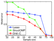
Figure 2: $1D$ contiguous regions: comparison between different methods for one (left), two (centre-left), three (centre-right) and four (right) regions.

Two dimensional contiguous regions. We repeated the experiment in the case that the sparsity pattern of $\beta^{*}\in{\mathbb{R}}^{20\times 20}$ consists of $2D$ rectangular regions. We considered either a single $5\times 5$ region, two regions ($4\times 4$ and $3\times 3$), three $3\times 3$ regions and four $3\times 2$ regions. Figure 4 shows the model error versus the sample size in this case. Figure 5 shows the original image and the images estimated by different methods for a sample size which is twice the model sparsity. Note that Grid-C is superior to both the Lasso and StructOMP and that StructOMP is outperformed by Lasso when the number of regions is more than two. This behavior is consistently confirmed by experiments in higher dimensions, not shown here for brevity.

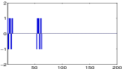
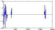
Figure 3: Two $1D$ contiguous regions: regression vector estimated by different models: $\beta^{*}$ (left), Lasso (centre-left), StructOMP (centre-right), Grid-C (right).

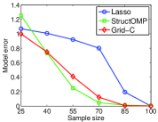
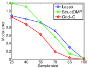
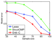
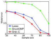
Figure 4: $2D$ contiguous regions: comparison between different methods for one (left), two (centre-left), three (centre-right) and four (right) regions.

Figure 5: $2D$-contiguous regions: model vector and vectors estimated by the Lasso, StructOMP and Grid-C (left to right), for one region (first group) and two regions (second group).

Background subtraction. We replicated the experiment from [9, Sec. 7.3] with our method. Briefly, the underlying model $\beta^{*}$ corresponds to the pixels of the foreground of a CCTV image. We measured the output as a random projection plus Gaussian noise. Figure 6-Left shows that, while the Grid-C outperforms the Lasso, it is not as good as StructOMP. We speculate that this result is due to the non uniformity of the values of the image, which makes it harder for Grid-C to estimate the model.

Image Compressive Sensing. In this experiment, we compared the performance of Tree-C on an instance of 2D image compressive sensing, following the experimental protocol of [9]. Natural images can be well represented with a wavelet basis and their wavelet coefficients, besides being sparse, are also structured as a hierarchical tree. We computed the Haar-wavelet coefficients of a widely used cameraman image. We measured the output as a random projection plus Gaussian noise. StructOMP and Tree-C, both exploiting the tree structure, were used to recover the wavelet coefficients from the measurements and compared to the Lasso. The inverse wavelet transform was used to reconstruct the images with the estimated coefficients. The recovery performances of the methods are reported in Figure 6-Right, which highlights the good performance of Tree-C.

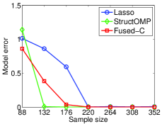
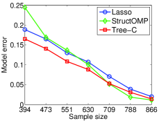
Figure 6: Model error for the background subtraction (left) and cameraman (right) experiments.

5 Conclusion

We proposed new families of penalties and presented a new algorithm and results on the class of structured sparsity penalty functions proposed by [12]. These penalties can be used, among else, to learn regression vectors whose sparsity pattern is formed by few contiguous regions. We presented a proximal method for solving this class of penalty functions and derived an efficient fixed-point method for computing the proximity operator of our penalty. We reported encouraging experimental results, which highlight the advantages of the proposed penalty function over a state-of-the-art greedy method [9]. At the same time, our numerical simulations indicate that the proximal method is computationally efficient, scaling linearly with the problem size. An important problem which we wish to address in the future is to study the convergence rate of the method and determine whether the optimal rate $O(\frac{1}{T^{2}})$ can be attained. Finally, it would be important to derive sparse oracle inequalities for the estimators studied here.

References

- [1] Argyriou, A., Evgeniou, T., and Pontil, M. Convex multi-task feature learning. Machine Learning, 73(3):243–272, 2008.
- [2] Bach, F. Structured sparsity-inducing norms through submodular functions. In Advances in Neural Information Processing Systems 23, pp. 118–126. 2010.
- [3] Baraniuk, R.G., Cevher, V., Duarte, M.F., and Hegde, C. Model-based compressive sensing. Information Theory, IEEE Transactions on, 56(4):1982–2001, 2010.
- [4] Beck, A. and Teboulle, M. A fast iterative shrinkage-thresholding algorithm for linear inverse problems. SIAM Journal of Imaging Sciences, 2(1):183–202, 2009.
- [5] Boyd, S. and Vandenberghe, L. Convex Optimization. Cambridge University Press, 2004.
- [6] Combettes, P.L. and Wajs, V.R. Signal recovery by proximal forward-backward splitting. Multiscale Modeling and Simulation, 4(4):1168–1200, 2006.
- [7] A. Gramfort and M. Kowalski. Improving M/EEG source localization with an inter-condition sparse prior, preprint, 2009.
- [8] H. Harzallah, F. Jurie, and C. Schmid. Combining efficient object localization and image classification. 2009. In IEEE International Symposium on Biomedical Imaging, 2009.
- [9] Huang, J., Zhang, T., and Metaxas, D. Learning with structured sparsity. In Proceedings of the 26th Annual International Conference on Machine Learning, pp. 417–424. ACM, 2009.
- [10] Jacob, L., Obozinski, G., and Vert, J.-P. Group lasso with overlap and graph lasso. In International Conference on Machine Learning (ICML 26), 2009.
- [11] Jenatton, R., Audibert, J.-Y., and Bach, F. Structured variable selection with sparsity-inducing norms. arXiv:0904.3523v2, 2009.
- [12] Micchelli, C.A., Morales, J.M., and Pontil, M. A family of penalty functions for structured sparsity. In Advances in Neural Information Processing Systems 23, pp. 1612–1623. 2010.
- [13] Micchelli, C.A., Shen, L., and Xu, Y. Proximity algorithms for image models: denoising. Inverse Problems, 27(4), 2011.
- [14] Moreau, J.J. Fonctions convexes duales et points proximaus dans un espace Hilbertien. Acad. Sci. Paris Sér. A Math., 255:2897–2899, 1962.
- [15] Mosci, S., Rosasco, L., Santoro, M., Verri, A., and Villa, S. Solving Structured Sparsity Regularization with Proximal Methods. Proc. of ECML, pages 418–433, 2010.
- [16] Nesterov, Y. Gradient methods for minimizing composite objective function. CORE, 2007.
- [17] G. Obozinski, B. Taskar, and M.I. Jordan. Joint covariate selection and joint subspace selection for multiple classification problems. Statistics and Computing, 20(2):1–22, 2010.
- [18] Opial, Z. Weak convergence of the sequence of successive approximations for nonexpansive operators. Bulletin American Mathematical Society, 73:591–597, 1967.
- [19] F. Rapaport, E. Barillot, and J.P. Vert. Classification of arrayCGH data using fused SVM. Bioinformatics, 24(13):i375–i382, 2008.
- [20] Rockafellar, R. T. Convex Analysis. Princeton University Press, 1970.
- [21] Tseng, P. On accelerated proximal gradient methods for convex-concave optimization. 2008. Preprint.
- [22] Z. Xiang, Y. Xi, U. Hasson, and P. Ramadge. Boosting with spatial regularization. In Y. Bengio, D. Schuurmans, J. Lafferty, C. K. I. Williams, and A. Culotta, editors, Advances in Neural Information Processing Systems 22, pages 2107–2115. 2009.
- [23] Yuan, M. and Lin, Y. Model selection and estimation in regression with grouped variables. Journal of the Royal Statistical Society, Series B, 68(1):49–67, 2006.
- [24] Zhao, P., Rocha, G., and Yu, B. Grouped and hierarchical model selection through composite absolute penalties. Annals of Statistics, 37(6A):3468–3497, 2009.