Spontaneous symmetry breaking in linearly coupled
disk-shaped Bose-Einstein condensates

Abstract

We study effects of tunnel coupling on a pair of parallel disk-shaped Bose-Einstein condensates with the self-attractive intrinsic nonlinearity. Each condensate is trapped in a combination of in-plane and transverse harmonic-oscillator potentials. It is shown that, depending on the self-interaction strength and tunneling coupling, the ground state of the system exhibits a phase transition which links three configurations: a symmetric one with equal numbers of atoms in the coupled condensates, an asymmetric configuration with a population imbalance (a manifestation of the macroscopic quantum self-trapping), and the collapsing state. A modification of the phase diagram of the system in the presence of vortices in the disk-shaped condensates is reported too. The study of dynamics around the stationary configurations reveals properties which strongly depend on the symmetry of the configuration.

10.1080/0026897YYxxxxxxxx 1362–3028 0026–8976 00 00 2011

1 Introduction

It has been predicted in many theoretical works [1] that two dilute symmetric Bose-Einstein condensates (BECs), which are weakly coupled by the tunneling of atoms across the separating potential barrier, can give rise to the macroscopic quantum self-trapping. In particular, in the case of attractive inter-atomic interactions, the ground state of the system shows a transition from the symmetric configuration (the Josephson regime), characterized by equal numbers of atoms in the coupled condensates, to an asymmetric state (the self-trapping regime), characterized by an imbalance in the number of atoms [1, 2]. In the case of repulsive interactions, the self-trapping occurs not in the ground state , but rather in the first antisymmetric excited state. In the latter case, the self-trapping was demonstrated in experiments with the condensate of ⁸⁷Rb atoms [3] (for a review, see Ref. [4]).

The self-trapping in the BEC loaded into the double-well potential is a manifestation of the general effect of the spontaneously symmetry breaking (SSB) in nonlinear systems. As said above, asymmetric states trapped in symmetric potentials are generated by SSB bifurcations from obvious symmetric or antisymmetric states, in the media with the attractive or repulsive intrinsic nonlinearity, respectively (the SSB under the action of competing attractive (cubic) and repulsive (quintic) terms was studied too, featuring closed bifurcation loops [5, 6]). In terms of BEC and other macroscopic quantum systems, the SSB may also be realized as a phase transition, which replaces the original symmetric ground state by a new asymmetric one, when the strength of the self-attractive nonlinearity exceeds a certain critical value. A transition of this type was actually predicted earlier in classical systems, viz., in a model of dual-core nonlinear optical fibers with the self-focusing Kerr nonlinearity [7]. In connection to the interpretation of the SSB as the phase transition, it may be identified as the transition of the first or second kind (alias subcritical or supercritical type of the SSB bifurcation), depending on the form of the nonlinearity, spatial dimension, and the presence or absence of an external periodic potential (an optical lattice) acting along the additional spatial dimension (if any) [8, 9].

Theoretical studies of the SSB in BECs were extended in various directions, especially for matter-wave solitons. In particular, the symmetry breaking of the solitons was predicted in various two-dimensional (2D) settings [8], including the spontaneous breaking of the skew symmetry of solitons and localized vortices trapped in double-layer condensates with mutually orthogonal orientations of quasi-one-dimensional optical lattices induced in the two layers [10]. A different variety of the 2D geometry, which gives rise to its own mode of the SSB, is based on a symmetric set of four potential wells [11]. Self-trapping of asymmetric states was also predicted in condensates formed of dipolar atoms, which interact via long-range forces [12], and in the context of the nonlinear Schrödinger equation with a general local nonlinearity [13]. The symmetry breaking is possible not only in linear potentials composed of two wells, but also in a similarly structured pseudopotentials, which are produced by a symmetric spatial modulation of the non-linearity coefficient, with two sharp maxima [14, 15].

Another generalization was developed for the SSB in two- [16] and three-component (spinor) [17] BEC mixtures, where the asymmetry of the density profiles in the two wells comes along with a difference in distributions of the different species. As concerns multi-component systems, the analysis of the SSB was also extended to Bose-Fermi mixtures [18].

On the other hand, it is commonly known that the self-attraction in BEC may cause collapse of the condensate in the form of a “bosenova” (in which case three-body recombinations become important, in addition to the usual two-body collisions [19]). Therefore, the SSB in BEC trapped in double-well (dual-core) potential may compete with the collapse. Recently, we have determined [20, 21] the domain of parameters of such a symmetric dual-core system above which the collapse occurs. In particular, the competition between the SSB and the onset of the collapse in a pair of parallel cigar-shaped atomic condensates weakly coupled by tunneling of atoms was investigated in Ref. [20]. Further, in Ref. [21], the SSB and collapse were studied in a quasi-1D bosonic Josephson junction made by a double-well potential in the axial direction, and by a harmonic potential in the radial directions.

In the present paper we consider a different setup, namely, a pair of parallel disk-shaped atomic condensates weakly-coupled by tunneling of atoms and confined by harmonic-oscillator potentials. This setup is ideal to analyze the interplay of the nonlinearity and tunnel coupling in the presence of vortices in both condensates [9]. In contrast to Ref. [9], which described this system by a pair of linearly-coupled 2D Gross-Pitaevskii equations (GPEs) with the cubic nonlinearity, and actually presented the analysis of the SSB only below the collapse threshold, in this work we use the more accurate system of equations with the nonpolynomial nonlinearity, specific to the 2D geometry [22], and the competition of the SSB with the onset of the collapse is one of main goals. After formulating the model in Section 2, we consider, in Section 3, the ground state of the system, which shows a phase transition between three possible configurations: a symmetric one, with equal numbers of atoms in the two coupled condensates, an asymmetric configuration with a population imbalance (the macroscopic self-trapping, in the present setting), and the collapsing state. Then, we perform a similar analysis for localized states carrying vorticity in each core, which changes the phase diagram of the system. Finally, we study the dynamics of the two disk-shaped condensates around the stationary configurations. Starting from a symmetric configuration, we predict small-amplitude Josephson-like oscillations, with periodic transfer of the population imbalance from one core to the other. Starting from an asymmetric configuration, we find, instead, large-amplitude oscillations, which preserve the population imbalance. The paper is concluded by summary and discussion of open problems in Section 4.

2 The model

2.1 The dimensional reduction from 3D to 2D

The starting point is the three-dimensional GPE for the mean-field wave function, $\psi(\mathbf{r},t)$, which describes BEC in two parallel identical disk-shaped traps separated by a potential barrier:

$$i\hbar{\frac{\partial}{\partial t}}\psi = \frac{1}{2}\left\{-\frac{\hbar}{m}\nabla^{2}+m\omega_{z}^{2}[(z-z_{0})^{2}+(z+z_{0})^{2}]\right\}\psi$$ (1)

$$+ W(x,y)\psi+\frac{4\pi\hbar^{2}a_{s}}{m}\left|\psi\right|^{2}\psi,$$

where $z$ is the coordinate transversal to the disks, $2z_{0}$ is the separation between their centers along the $z$-direction, the two harmonic potentials with frequency $\omega_{z}$ account for the transverse trapping of atoms in each disk, and $W(x,y)$ is the potential acting in the disk plane (it is assumed to be identical for both disks). As usual, $a_{s}$ is the $s$-wave inter-atomic scattering length [23].

The first objective is to reduce Eq. (1) to a system of linearly coupled equations for 2D wave functions pertaining to the separate disks, $\Phi_{1,2}$. To this end, we modify the approach developed for the system of two parallel quasi-1D “cigars” in Ref. [20], adopting a superposition of two single-disk ansätze:

$$\psi(\mathbf{r},t) = \pi^{-1/4}\left[\exp\left(-\frac{\left(z-z_{0}\right)^{2}}{2\eta_{1}(x,y,t)^{2}}\right)\frac{\Phi_{1}(x,y,t)}{\sqrt{\eta_{1}(x,y,t)}}\right.$$ (2)

$$\left.+\exp\left(-\frac{\left(z+z_{0}\right)^{2}}{2\eta_{2}(x,y,t)^{2}}\right)\frac{\Phi_{2}(x,y,t)}{\sqrt{\eta_{2}(x,y,t)}}\right],$$

where $\eta_{1}(x,y,t)$ and $\eta_{2}(x,y,t)$ are the thicknesses of the two disks along the $z$ axis, and the 1D part of each wave function is normalized to unity.

We proceed by substituting ansatz (2) into the Lagrangian corresponding to Eq. (1),

$$L=\frac{1}{2}\int d^{3}\mathbf{r}\Big{\{}i\hbar\Big{(}{\frac{\partial\psi^{\ast}}{\partial t}}\psi-{\frac{\partial\psi}{\partial t}}\psi^{\ast}\Big{)}+\frac{\hbar^{2}}{m}|\nabla\psi|^{2}$$

$$+m\omega_{z}^{2}[(z-z_{0})^{2}+(z+z_{0})^{2}]|\psi|^{2}$$

$$+2W(x,y)|\psi|^{2}+\frac{4\pi\hbar^{2}a_{s}}{m}|\psi|^{4}\Big{\}}:.$$ (3)

The underlying assumption is that distance $2z_{0}$ between the disks is essentially larger than the size $a_{z}=\sqrt{\hbar/(m\omega_{z})}$ of the transverse confinement in each of them, $2z_{0}\gg a_{z}$. Due to this condition, the part of the Lagrangian, which accounts for the tunneling and is produced by the overlap of the two components of the wave function in ansatz (2), if substituted into Lagrangian (3), takes the following form:

$$L_{\mathrm{T}}=-K\int\left[\Phi_{1}(x,y)\Phi_{2}^{\ast}(x,y)+\Phi_{1}^{\ast}(x,y)\Phi_{2}(x,y)\right]dxdy,$$

where the effective coupling coefficient is defined as

$$K=\hbar\omega_{z}{\frac{z_{0}^{2}}{a_{z}^{2}}}\exp\left(-\frac{z_{0}^{2}}{a_{z}^{2}}\right).$$ (4)

In fact, the main contribution to the linear coupling (tunneling) comes from region $z^{2}\lesssim\eta_{1,2}^{2}$ around the midpoint between the disks. In that region, the transverse-confinement radius is determined by the ground-state wave function of the 1D harmonic oscillator, which has characteristic length $a_{z}$ in the $z$ direction.

Finally, the effective dynamical equations for the two linearly coupled disks ($n=1,2)$ are written as

$$i{\frac{\partial}{\partial t}}\Phi_{n} = \Big{[}-{\frac{1}{2}}\nabla_{\bot}^{2}+W(x,y)+g{\frac{|\Phi_{n}|^{2}}{\eta_{n}}}$$ (5)

$$+{\frac{1}{4}}\left({\frac{1}{\eta_{n}^{2}}}+\eta_{n}^{2}\right)\Big{]}\Phi_{n}-\kappa\ \Phi_{3-n}\;,$$

where the scaled interaction strength is $g\equiv\sqrt{2\pi}\gamma$, with

$$\gamma=2Na_{s}/a_{z},$$ (6)

the scaled linear coupling is

$$\kappa=K/(\hbar\omega_{z}),$$ (7)

and the respective axial widths are determined by algebraic equations,

$$\eta_{n}^{4}=1+g|\Phi_{n}|^{2}\eta_{n},\;.$$ (8)

Notice that in Eqs. (5) and (8) we have used scaled variables, viz., the length measured in units of $a_{z}=\sqrt{\hbar/(m\omega_{z})}$, time in units of $\omega_{z}^{-1}$, and energy in units of $\hbar\omega_{z}$.

Exact solutions to Eqs. (8) can be found by way of the Cardano formula,

$$\eta_{n} = \pm{\frac{1}{2}}\sqrt{\frac{A_{n}^{2}-12}{3A_{n}}}$$ (9)

$$+ {\frac{1}{2}}\sqrt{-{\frac{A_{n}^{2}-12}{3A_{n}}}\pm 2g|\Phi_{n}|^{2}\left(\frac{A_{n}^{2}-12}{3A_{n}}\right)^{-1/2}}\;,$$

where the upper and lower signs correspond, respectively, to $g>0$ and $g<0$, and

$$A_{n}\equiv\left({3/2}\right)^{1/3}\left(9g^{2}|\Phi_{n}|^{4}+\sqrt{3}\sqrt{256+27g^{4}|\Phi_{n}|^{8}}\right)^{1/3}\;.$$ (10)

2.2 Properties of the 2D model

Thus, we have reduced the initial 3D problem, based on Eq. (1), to the 2D problem for the set of wave functions of the BECs trapped in the two disks, which obey Eqs. (5) and (8). To stabilize 2D solitons and vortices, we choose the in-plane potential as that of the 2D harmonic oscillator,

$$W\left(x,y\right)=\frac{1}{2}\lambda^{2}(x^{2}+y^{2}),$$ (11)

where $\lambda$ is the adimensional frequency of the planar confinement. The system conserves the total number of atoms in the two disks, i.e., $N_{1}(t)+N_{2}(t)=2\$(in the scaled units), where

$$N_{n}=\int|\Phi_{n}(x,y,t)|^{2}dxdy\quad\quad(n=1,2)\;.$$

Also conserved are the total energy and angular momentum.

It is relevant to mention that the (effectively) two-dimensional self-attractive condensate, trapped in a periodic optical-lattice potential, features not only the collapse, when its norm exceeds the corresponding critical value, but also delocalization, when the norm falls below a certain threshold (the latter effects is also known in other dimensions) [24]. In the present setting, the delocalization does not occur, as we consider the situation with the harmonic-oscillator potentials confining the condensates in all directions.

Vortex-soliton solutions to Eqs. (5) are sought for as

$$\Phi_{n}(r,\theta,t)=\phi_{n}(r,t)\ e^{iS\theta}\;,$$

where $r$ and $\theta$ are the polar coordinates in the $\left(x,y\right)$ plane, and $S$ is the integer vorticity. In this way, Eqs. (5) can be reduced to coupled nonpolynomial Schrödinger equations in the radial direction,

$$i{\frac{\partial}{\partial t}}\phi_{n} = \frac{1}{2}\Big{[}-\left({\frac{\partial^{2}}{\partial r^{2}}}+{\frac{1}{r}}{\frac{\partial}{\partial r}}\right)+{\frac{S^{2}}{r^{2}}}+\lambda^{2}r^{2}+2g{\frac{|\phi_{n}|^{2}}{\eta_{n}}}$$ (12)

$$+ {\frac{1}{2}}\left({\frac{1}{\eta_{n}^{2}}}+\eta_{n}^{2}\right)\Big{]}\phi_{n}-\kappa\ \phi_{3-n}~{}.$$

Further, stationary states are then obtained by setting $\phi_{n}(r,t)=u_{n}(r)\ e^{-i\mu_{n}t},$ with real functions $u_{n}$, which obey a system of stationary radial equations,

$$\mu_{n}u_{n} = \frac{1}{2}\Big{[}-\left({\frac{\partial^{2}}{\partial r^{2}}}+{\frac{1}{r}}{\frac{\partial}{\partial r}}\right)+{\frac{S^{2}}{r^{2}}}+\lambda^{2}r^{2}+2g{\frac{u_{n}^{2}}{\eta_{n}}}$$

$$+ {\frac{1}{2}}\left({\frac{1}{\eta_{n}^{2}}}+\eta_{n}^{2}\right)\Big{]}u_{n}-\kappa u_{3-n}\;,$$

while widths $\eta_{1,2}$ are still determined by Eqs. (8), with $\left|\Phi_{1,2}\right|^{2}$ replaced by $u_{1,2}^{2}$.

As said above, the main objective of the work is to predict the SSB of the symmetric solitons, with $u_{1}\left(r\right)=u_{2}\left(r\right)$, $\eta_{1}=\eta_{2}$. In the system of two linearly coupled GPEs with the usual cubic nonlinearity, this problem was studied in Ref. [9]. Here, we seek for stationary solutions by means of direct simulations of the time-dependent cylindrically-symmetric coupled 2D equations (12), using a finite-difference Crank-Nicholson algorithm in the imaginary time [25]. The initial conditions were taken as

$$\Phi_{n}(r,t=0)=C_{n}\ r^{S}\ \exp\left(-\lambda r^{2}/2\right),$$ (13)

where $C_{n}$ ($n=1,2$) are normalization constants. Note that Eq. (13) gives the exact quantum-mechanical wave function of the stationary vortex configuration in the absence of the nonlinearity ($g=0$) and linear coupling ($\kappa=0$). In our numerical simulations we choose $C_{1}\neq C_{2}$, but with $C_{1}$ taken very close to $C_{2}$, to initiate the development of the symmetry breaking, if it possible. In particular, the norms of functions $\Phi_{1}(r,t=0)$ and $\Phi_{2}(r,t=0)$ are taken as $1.01$ and $0.99$, respectively.

3 Numerical results

3.1 The ground state and vortices

In Fig. 1 we plot the norms $N_{1}$ and $N_{2}$ (solid and dashed lines) of the two coupled condensates, with zero vorticity, $S=0$, in the course of the evolution of in the imaginary time, by choosing $\gamma=-0.4$ [recall $\gamma$ is defined in Eq. (6), $\gamma<0$ corresponding to the attractive interatomic interactions], and slightly asymmetric initial conditions (i.e. slightly imbalanced populations). As shown in the figure, with $\kappa=0.25$ (the upper panel) the symmetry is restored during the time evolution, while with $\kappa=0.15$ (the lower panel) the asymmetry is strongly enhanced towards a finite population imbalance.

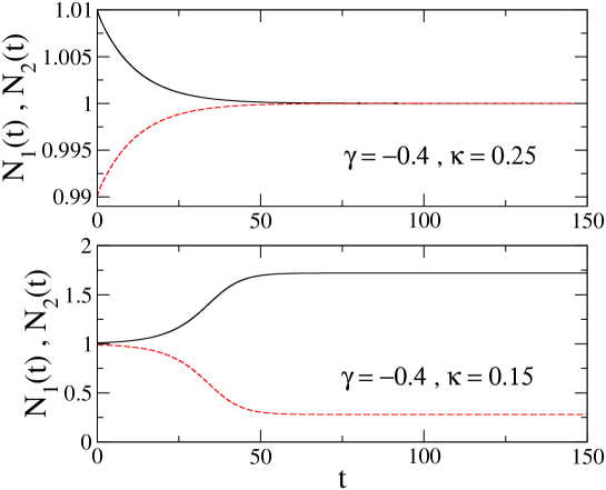
Figure 1: (Color online) Norms $N_{1}$ and $N_{2}$ (solid and dashed lines) of the ground (zero-vorticity, $S=0$) state trapped in the two parallel disks, in the course of the evolution in imaginary time. The nonlinearity coefficient is $\gamma=-0.4$, while the coupling constant is $\kappa=0.25$ (upper panel) and $\kappa=0.15$ (lower panel). The adimensional notation corresponds to the length measured in units of $a_{z}=\sqrt{\hbar/(m\omega_{z})}$, time in units of $\omega_{z}$, and energy in units of $\hbar\omega_{z}$. Recall that $\gamma\$and $\kappa\$are defined by Eqs. (6) and (7), respectively.

In the framework of the 2D description, the factorized ansatz (2) yields the time-dependent radial density profile, $\rho_{n}(r,t)=|\Phi_{n}(r,t)|^{2},$ and its axial counterpart,

$$\rho_{n}(z,t)=2\sqrt{\pi}\int_{0}^{\infty}\frac{rdr}{\eta_{n}(r,t)}e^{-z^{2}/\eta_{n}(r,t)^{2}}|\Phi_{n}(r,t)|^{2}\;.$$ (14)

In Fig. 2 the corresponding final (stationary) density profiles are displayed in the two disks, by solid and dashed lines. In the upper panels, the density profiles of the symmetric state are fully superimposed, while in the lower panels they are clearly distinguishable, for the asymmetric mode.

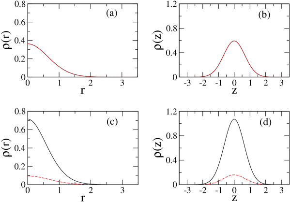
Figure 2: (Color online) Stationary density profiles of the ground state ($S=0$) in the two disks (solid and dashed lines), corresponding to the cases shown in Fig. (1). The upper panels: radial density profiles $\rho(r)$ (a), and axial density profiles $\rho(z)$, see Eq. (14), (b), for $\gamma=-0.4$ and $\kappa=0.25$. Lower panels: the radial profiles (c) and the axial profiles (d) for $\gamma=-0.4$ and $\kappa=0.15$. Units are the same as in Fig. 1.

Results of a systematic analysis, generated by varying parameters $\gamma$ and $\kappa$, are summarized in Fig. 3. Here we show the phase diagram generated by the linearly-coupled system of 2D equations (12), with $S=0$, in the parameter plane. As explained also in the the caption to the figure, in regions “symmetric” and “SSB” the system supports, respectively, stable symmetric and asymmetric stationary solutions. In region “collapse”, the imaginary-time dynamics evolves towards a configuration with a zero-length axial width (in one or both disks). Notice that, on the right side of the vertical dashed line in Fig. 3 (i.e., at $|\gamma|>1.07$), the system always suffers the collapse, as in that region the nonlinearity strength exceeds the critical value leading to the onset of the collapse.

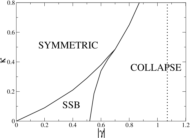
Figure 3: The phase diagram of the linearly-coupled system of 2D equations (12) with $S=0$ (the ground state). In regions “symmetric” and “SSB”, the system supports, respectively, stable symmetric [$u_{1}(r)=u_{2}(r)$] and asymmetric [$u_{1}(r)\neq u_{2}(r)$] stationary solutions. The collapse takes place in the eponymous region. The system always suffers the collapse to the right of the vertical dashed line. Units are as in Fig. 1.

The density profiles of the vortical states with $S=1$ in both disks are displayed in Fig. 4, by means of the solid and dashed lines. The left panels of the figure clearly show the impact of the vorticity on the radial profiles $\rho(r)$, which vanish at $r\rightarrow 0$. The figure also shows that, as expected, the transition to the asymmetric configuration follows reducing $\kappa$.

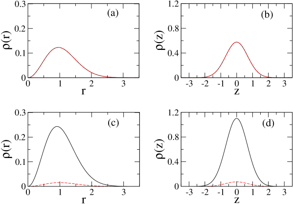
Figure 4: (Color online) Stationary density profiles of vortices with $S=1$ in the two disks (solid and dashed lines). Upper panels: (a) radial density profiles $\rho(r)$ (a) and axial density profiles $\rho(z)$ (b) for $\gamma=-0.4$ and $\kappa=0.2$. Lower panels: radial profiles (c) and axial profiles (d) for $\gamma=-0.05$ and $\kappa=0.15$. The units are as in Fig. 1.

For the modes with $S=1$, the phase diagram of the linearly-coupled system of equations (12) in the parameter plane of $(\gamma,\kappa)$ is displayed in Fig. 5. Comparing Figs. 3 and 5, we conclude that the “collapse region” is slightly reduced at the nonzero vorticity. In this case, the system always collapses at $|\gamma|>1.36$.

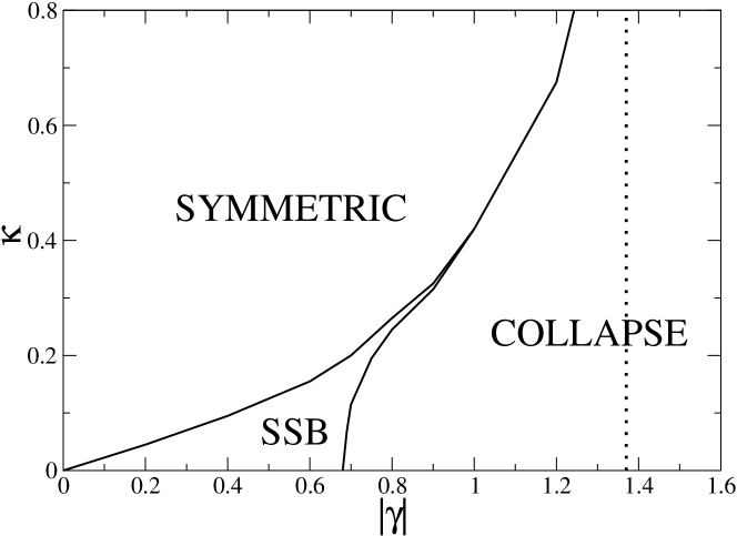
Figure 5: The phase diagram of the linearly-coupled system of Eqs. (12) for the vortex modes with $S=1$. In regions “symmetric” and “SSB”, the system supports, respectively, stable symmetric [$u_{1}(r)=u_{2}(r)$] and asymmetric [$u_{1}(r)\neq u_{2}(r)$] stationary solutions. The collapse takes place in the eponymous region. The system always collapses on the right side of the vertical dashed line. Units are the same as in Fig. 1.

The SSB can be characterized by the imbalance (asymmetry) parameter,

$$\zeta(t)=\frac{N_{1}(t)-N_{2}(t)}{N_{1}(t)+N_{2}(t)}=\frac{N_{1}(t)-N_{2}(t)}{N}\;.$$ (15)

The competition between the symmetry breaking and collapse is further illustrated in Fig. 6 by plots of $\zeta$ versus $\gamma$ for a relatively weak linear coupling, $\kappa=0.1$. In this figure, $\zeta$ is the asymptotic value produced by the imaginary-time evolution in the framework of Eqs. (12) with initial value $\zeta(0)=0.01$. The curves in Fig. 6 feature a leap (represented by vertical segments) from the symmetric configuration with $\zeta=0$ to the asymmetric one with $\zeta\neq 0$. Actually, the transition to asymmetric states in the present model always happens by a leap, i.e., the symmetry-breaking bifurcation is always subcritical, similar to the situation in the coupled equations with the self-attractive cubic nonlinearity [8]. The figure shows that, at fixed $\kappa$, both the SSB and collapse happen at higher values of $|\gamma|$ in the case of $S=1$, with respect to $S=0$.

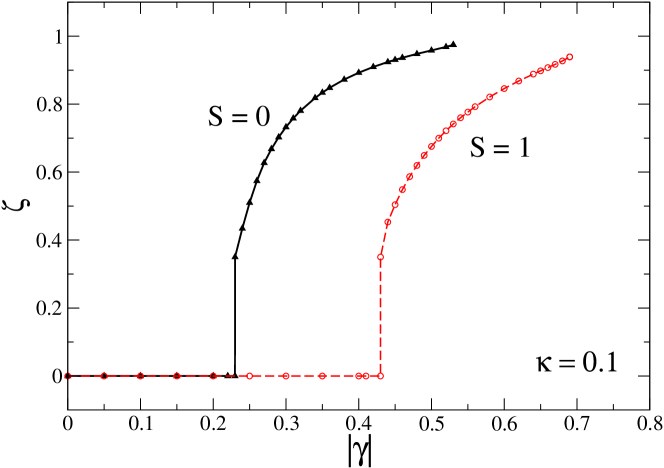
Figure 6: (Color online) The imbalance parameter, defined as per Eq. (15), as a function of interaction strength $\gamma$, for $S=0$ (filled triangles connected by the solid line), and $S=1$ (open circles connected by the dashed line), for $\kappa=0.1$. The curves terminate at the collapse points. Units are as in Fig. 1.

3.2 Real-time dynamics

In the above subsections we have reported results of the imaginary-time simulations, which produce the stationary solutions. The next step is to test the stability of the modes by solving Eqs. (12) in real time. In Fig. 7 we display the real-time dynamics of the imbalance parameter, $\zeta(t)$, of the system with $\kappa=0.1$ for $S=0$. The initial value is $\zeta(0)=0.01$. In the upper panel, we chose $\gamma=-0.1$, which corresponds to a stationary symmetric configuration, while in the lower panel we set $\gamma=-0.4,$ which pertains to the asymmetric mode.

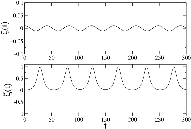
Figure 7: The real-time dynamics of the imbalance defined as per Eq. (15), for $\kappa=0.1$ and $S=0$. The upper and lower panels correspond, respectively, to values of the interaction strength $\gamma=-0.1$ and $\gamma=-0.4$. The initial imbalance is $\zeta(0)=0.01$. Units are as in Fig. 1.

Figure 7 shows that the dynamics are completely different in the two cases. With the initial imbalance $\zeta(0)=0.01$ in both cases, $\zeta(t)$ remains small in the course of the oscillations around the stationary symmetric configuration, changing its sign periodically. Actually, $\zeta(t)$ oscillates harmonically around the $\zeta=0$. In the case of the stationary asymmetric configuration, the imbalance $\zeta(t)$ periodically assumes very large values, but it does not change the sign; actually, $\zeta(t)$ oscillates around a mean value, $\bar{\zeta}\simeq 0.5$. Note that the value of $\zeta$ obtained asymptotically with these parameters ($\kappa=0.1$ and $\gamma=-0.4$) in the imaginary-time simulations is $\zeta=0.89$, see Fig. 6.

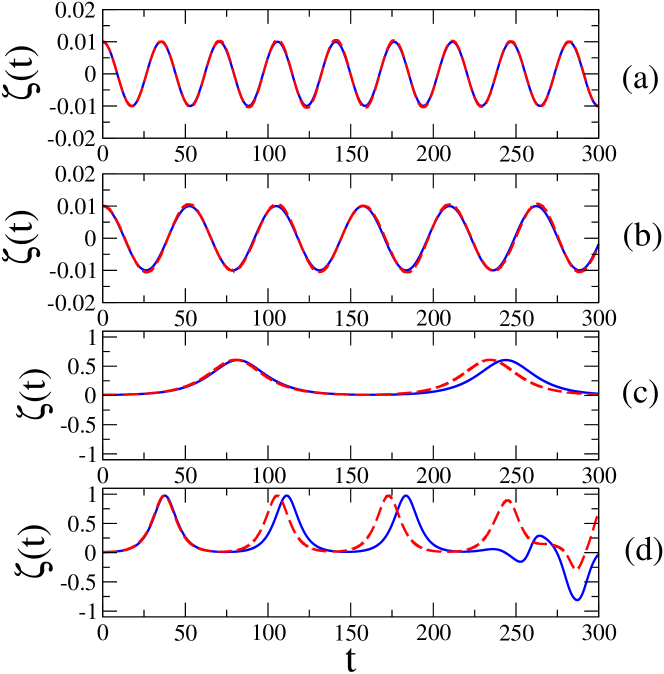
Figure 8: (Color online) The real-time dynamics of the imbalance, defined by Eq. (15), for the vortex modes with $S=1$, at $\kappa=0.1.$ Four values of the interaction strength $\gamma$ are considered: (a) $\gamma=-0.1$, (b) $\gamma=-0.3$, (c) $\gamma=-0.5$, (d) $\gamma=-0.7$. The initial imbalance is $\zeta(0)=0.01$, in all the cases. The solid lines are obtained by solving Eqs. (5) for the axially-symmetric initial conditions (16) with $\delta=1$, while the dashed lines are generated by the initial conditions with $\delta=1.1$, which break the azimuthal symmetry. Units are as in Fig. 1.

In Fig. 8 we plot the evolution of $\zeta(t)$ for $S=1$. It is important to stress that when the stability of the vortex solutions is tested against perturbations in real time, it is necessary to study the stability of the vortex against azimuthal perturbations, which may lead to splitting of the vortex that might seem stable in axially symmetric simulations [26]. For this reason, we employed full equations (5) to study the real-time dynamics of the vortices, considering both axially-symmetric initial conditions and those breaking the azimuthal symmetry. The general initial conditions used for the simulations of Eq. (5) are

$$\Phi_{1}(x,y,t = 0)=(x+iy)e^{-(x^{2}+\delta y^{2})/2}\;,$$

$$\Phi_{2}(x,y,t = 0)=(x+iy)e^{-(x^{2}+\delta y^{2})/2}\;.$$ (16)

We set $\delta=1$ for the symmetric configurations, and $\delta=1.1$ for ones with the broken azimuthal symmetry. Notice that $\Phi_{1}(x,y,t=0)$ is normalized to $N_{1}(0)=1.01$ and $\Phi_{2}(x,y,t=0)$ to $N_{2}(0)=0.99$. In Fig. 8 the two upper panels [(a) with $\gamma=-0.1$ and (b) with $\gamma=0.3$] correspond to stationary symmetric configurations (the Josephson regime), with $\kappa=0.1$ (see Fig. 6). The results displayed in these two panels of Fig. 8 show (the solid lines versus the dashed ones) that the additional azimuthal perturbation has no appreciable effects in the dynamics, apart from a slight dephasing. The third panel of Fig. 8 [(c), with $\gamma=-0.5$] corresponds to a stationary asymmetric vortex (in the self-trapping regime). Here we find large-amplitude oscillations without a change in the sign of the population imbalance, $\zeta(t)$. The solution with the unbroken azimuthal symmetry (the dashed line) has a period of oscillations very close to that observed in the solution with the azimuthal perturbation (the solid line). In any case, we conclude that the asymmetric vortex with $\kappa=0.1$, $\gamma=-0.5$ and $S=1$ is dynamically stable. Finally, in the bottom panel of Fig. 8 we plot $\zeta(t)$ for parameters $S=1$, $\kappa=0.1$ and $\gamma=-0.7$, which are at the border of the collapse region (see Fig. 6). The panel shows that the solution is unstable (and eventually suffers the collapse). Here, the main difference between solid and dashed curves is the time after which $\zeta(t)$ displays the instability, which may be identified as the instant at which $\zeta(t)$ changes its sign for the first time. We observe that the instability with respect to the azimuthal perturbations can produce an additional border inside both the symmetric and asymmetric domains in Fig. 5. We did not aim to produce this border in an exact form, as it is a computationally expensive objective.

4 Conclusions and open problems

We have studied the dynamics of the self-attractive BEC in tunnel-coupled disk-shaped traps, by means of systematic simulations of the coupled nonpolynomial Schrödinger equations derived from the 3D Gross-Pitaevskii equation. In this way, we have investigated the phase diagram of the system as a function of the interaction strength ($\gamma$) and tunneling coupling. We have found that borders of different domains in the phase diagram depend on vorticity $S$ of the localized modes: both the SSB (spontaneous symmetry breaking) and collapse happen at larger values of $\gamma$ in the case of $S=1$ case with respect to the ground state ($S=0$). We have also studied the dynamics of the two disk-shaped condensates around the stationary configurations. Small-amplitude harmonic oscillations, showing a periodic transfer of atoms between the condensates, take place around the stable symmetric configurations. Instead, large-amplitude oscillations without the change of the sign of the imbalance between the two condensates occur around the perturbed asymmetric configurations.

There are many interesting open problems about Bose-Einstein condensates coupled by tunneling we want to face in the next future. In particular, we plan to investigate quasi one-dimensional and quasi two-dimensional Bose-Einstein condensates in nonlinear lattices (i.e. with space-dependent interaction strength) [27] by using the nonpolynomial Schrödinger equations. Moreover, we want to analyze the signatures of classical and quantum chaos [28] in these double-well configurations. Finally, we aim to calculate analytically the coupling tunneling energy of bosons by means of the WKB semiclassical quantization [29] and comparing it with the numerical results of the Gross-Pitaevskii equation.

LS thanks Luciano Reatto for 9 years of fruitful scientific collaboration at the Physics Department of the University of Milano.

References

- [1] G. J. Milburn, J. Corney, E. M. Wright, and D. F. Walls, Phys. Rev. A 55, 4318 (1997); A. Smerzi, S. Fantoni, S. Giovanazzi, and S. R. Shenoy, Phys. Rev. Lett. 79, 4950 (1997); S. Raghavan, A. Smerzi, S. Fantoni, and S. R. Shenoy, Phys. Rev. A 59, 620 (1999); K. W. Mahmud, H. Perry, and W. P. Reinhardt, Phys. Rev. A 71, 023615 (2005); E. Infeld, P. Zin, J. Gocałek, and M. Trippenbach, Phys. Rev. E 74, 026610 (2006); G. Theocharis, P. G. Kevrekidis, D. J. Frantzeskakis, and P. Schmelcher, Phys. Rev. E 74, 056608 (2006); G. L. Alfimov and D. A. Zezyulin, Nonlinearity 20, 2075 (2007).
- [2] A. J. Leggett, Quantum Fluids (Oxford University Press, Oxford) (2006).
- [3] M. Albiez, R. Gati, J. Fölling, S. Hunsmann, M. Cristiani, and M. K. Oberthaler, Phys. Rev. Lett. 95, 010402 (2005),
- [4] O. Morsch and M. Oberthaler, Rev. Mod. Phys. 78, 179 (2006); R. Gati and M. Oberthaler, J. Phys. B. 40, R61 (2007)
- [5] L. Albuch and B. A. Malomed, Mathematics and Computers in Simulation 74, 312 (2007); Z. Birnbaum and B. A. Malomed, Physica D 237, 3252 (2008).
- [6] N. Dror and B. A. Malomed, Physica D 240, 526 (2011).
- [7] A. W. Snyder, D. J. Mitchell, L. Poladian, D. R. Rowland, and Y. Chen, J. Opt. Soc. Am. B 8, 2102 (1991).
- [8] A. Gubeskys and B. A. Malomed, Phys. Rev. A 75, 063602 (2007); M. Matuszewski, B. A. Malomed, and M. Trippenbach, ibid. 75, 063621 (2007); M. Trippenbach, E. Infeld, J. Gocałek, M. Matuszewski, M. Oberthaler, and B. A. Malomed, ibid. A 78, 013603 (2008).
- [9] A. Gubeskys and B. A. Malomed, Phys. Rev. A 76, 043623 (2007).
- [10] T. Mayteevarunyoo and B. A. Malomed, J. Opt. A: Pure Appl. Opt. 11, 094015 (2009).
- [11] C. Wang, G. Theocharis, P. G. Kevrekidis, N. Whitaker, K. J. H. Law, D. J. Frantzeskakis, and B. A. Malomed, Phys. Rev. E 80, 046611 (2009).
- [12] B. Xiong, J. Gong, H. Pu, W. Bao, and B. Li, Phys. Rev. A 79, 013626 (2009).
- [13] A. Sacchetti, Phys. Rev. Lett. 103, 194101 (2009).
- [14] T. Mayteevarunyoo, B. A. Malomed, and G. Dong, Phys. Rev. A 78, 053601 (2008); C. Wang, P. G. Kevrekidis, N. Whitaker, D. J. Frantzeskakis, S. Middelkamp, and P. Schmelcher, Physica D 238, 1362 (2009); N. Dror and B. A. Malomed, Phys. Rev. A 83, 033828 (2011).
- [15] Y. V. Kartashov, B. A. Malomed, and L. Torner, Rev. Mod. Phys. 83, 247 (2011).
- [16] C. Wang, P. G. Kevrekidis, N. Whitaker and B. A. Malomed, Physica D 327, 2922 (2008); I. I. Satija, R. Balakrishnan, P. Naudus, J. Heward, M. Edwards, and C. W. Clark, Phys. Rev. E 79, 033616 (2009); W. Wang, J. Phys. Soc. Jpn. 78, 094002 (2009); C. Lee, Phys. Rev. Lett. 102, 070401 (2009),
- [17] C. Wang, P. G. Kevrekidis, N. Whitaker, T. J. Alexander, D. J. Frantzeskakis, and P. Schmelcher, J. Phys. A Math. Theor. 42, 035201 (2009); B. Juliá-Diaz, M. Guilleumas, M. Lewenstein, A. Polls, and A. Sanpera, Phys. Rev. A 80, 023616 (2009); B. Juliá-Diaz, M. Mele-Messeguer, M. Guilleumas, and A. Polls, Phys. Rev. A 80, 043622 (2009).
- [18] S. F. Caballero-Benítez, E A Ostrovskaya, M. Gulácsí, and Yu. S. Kivshar, J. Phys. B 42, 215308 (2009); S. K. Adhikari, B. A. Malomed, L. Salasnich, and F. Toigo, Phys. Rev. A 81, 053630 (2010).
- [19] E. A. Donley, N. R. Claussen, S. L. Cornish, J. L. Roberts, E. A. Cornell, and C. E. Wieman, Nature 412, 295 (2001).
- [20] L. Salasnich, B. A. Malomed, and F. Toigo, Phys. Rev. A 81, 045603 (2010).
- [21] G. Mazzarella and L. Salasnich, Phys. Rev. A 82, 033611 (2010).
- [22] L. Salasnich, A. Parola, and L. Reatto, Phys. Rev. A 65, 043614 (2002).
- [23] L. P. Pitaevskii and A. Stringari, Bose-Einstein Condensation (Clarendon Press: Oxford, 2003).
- [24] B. B. Baizakov and M. Salerno, Phys. Rev. A 69, 013602 (2004); H. A. Cruz, V. A. Brazhnyi, V. V. Konotop, and M. Salerno, Physica D 238, 1372 (2009).
- [25] E. Cerboneschi, R. Mannella, E. Arimondo, and L. Salasnich, Phys. Lett. A 249, 495 (1998); G. Mazzarella and L. Salasnich, Phys. Lett. A 373, 4434 (2009).
- [26] D. Mihalache, D. Mazilu, B.A. Malomed, and F. Lederer, Phys. Rev. A 73, 043615 (2006).
- [27] Y.V. Kartashov, B.A. Malomed, and L. Torner, Rev. Mod. Phys. 83, 247 (2011).
- [28] L. Salasnich, Phys. Rev. D 52, 6189 (1995); L. Salasnich, Mod. Phys. Lett. A 12, 1473 (1997); A.R. Kolovsky and A. Buchleitner, Europhys. Lett. 68 632 (2004); C. Weiss and N. Teichmann, Phys. Rev. Lett. 100, 140408 (2008).
- [29] M. Robnik and L. Salasnich, J. Phys. A: Math. Gen. 30, 1711 (1997); M. Robnik and L. Salasnich, J. Phys. A: Math. Gen. 30, 1719 (1997); G. Alvarez, J. Math. Phys. 45, 3095 (2004); A.V. Turbiner, Int. J. Mod. Phys. A 25, 647-658 (2010).