Spectral properties of a 2D scalar wave equation with
1D-periodic coefficients: application to SH elastic waves

Abstract

The paper provides a rigorous analysis of the dispersion spectrum of SH (shear horizontal) elastic waves in periodically stratified solids. The problem consists of an ordinary differential wave equation with periodic coefficients, which involves two free parameters $\omega$ (the frequency) and $k$ (the wavenumber in the direction orthogonal to the axis of periodicity). Solutions of this equation satisfy a quasi-periodic boundary condition which yields the Floquet parameter $K$. The resulting dispersion surface $\omega(K,k)$ may be characterized through its cuts at constant values of $K,~{}k$ and $\omega$ that define the passband (real $K$) and stopband areas, the Floquet branches and the isofrequency curves, respectively. The paper combines complementary approaches based on eigenvalue problems and on the monodromy matrix $\mathbf{M}$. The pivotal object is the Lyapunov function $\Delta\left(\omega^{2},k^{2}\right)\equiv\frac{1}{2}\mathrm{trace}\mathbf{M}=\cos K$ which is generalized as a function of two variables. Its analytical properties, asymptotics and bounds are examined and an explicit form of its derivatives obtained. Attention is given to the special case of a zero-width stopband. These ingredients are used to analyze the cuts of the surface $\omega(K,k).$ The derivatives of the functions $\omega(k)$ at fixed $K$ and $\omega(K)$ at fixed $k$ and of the function $K(k)$ at fixed $\omega$ are described in detail. The curves $\omega(k)$ at fixed $K$ are shown to be monotonic for real $K,$ while they may be looped for complex $K$ (i.e. in the stopband areas). The convexity of the closed (first) real isofrequency curve $K(k)$ is proved thus ruling out low-frequency caustics of group velocity. The results are relevant to the broad area of applicability of ordinary differential equation for scalar waves in 1D phononic (solid or fluid) and photonic crystals.

1 Introduction

The wave equation with periodic coefficients is ubiquitous in physics and engineering. Its applications in acoustics of solids have gained a new momentum since the introduction of artificial periodic materials such as phononic crystals. A common mathematical framework is the Floquet-Bloch theory of partial differential equations with periodic coefficients [16]. It does not however yield many explicit results for the general case of 2D or 3D periodicity and vector waves. The notable exception allowing an explicit analysis is the case of 1D periodicity and scalar waves which is governed by Hill’s equation [17]. The spectral properties of Hill’s equation are very well understood for the situation where the wave propagates along some fixed direction (parallel to the periodicity axis or not). This case implies a single spectral parameter. The objective of the present paper is to take on a broader perspective of arbitrary (2D) propagation of scalar waves in 1D periodic media. This setup implicates dependence on two spectral parameters and thus leads to more elaborate wave spectral properties. The specific problem to be addressed is described next.

Consider SH (shear horizontal) wave motion of the form $u_{z}\left(x,y,t\right)=U(y)\exp\left[i\left(kx-\omega t\right)\right]$ which travels in the symmetry plane $XY$ of a stratified monoclinic elastic solid with periodic density $\rho\left(y\right)=\rho\left(y+T\right)$ and stiffness $c_{ijkl}\left(y\right)=c_{ijkl}\left(y+T\right)$. The elastodynamic equation yields a second-order ordinary differential equation for the amplitude $U(y),$

$$\partial_{j}\left(c_{ijkl}\partial_{l}u_{k}\right)=\rho\ddot{u}_{i}\ \Rightarrow\left(c_{44}U^{\prime}+ikc_{45}U\right)^{\prime}+ik\left(c_{45}U^{\prime}+ikc_{55}U\right)=-\rho\omega^{2}U,$$ (1)

where $\partial_{1}\equiv\partial/\partial x,\ \partial_{2}\equiv\partial/\partial y,\ ^{\prime}\equiv d/dy$ and Voigt’s indices $4=yz,$ $5=xz$ are used [3]. It is convenient to pass from $U$ to $u=Ue^{i\varphi}$ with $\varphi\left(y\right)=ik\int^{y}\left(c_{45}/c_{44}\right)\mathrm{d}y$ which reduces (1)₂ to the Sturm-Liouville form

$$\left(\mu_{1}(y)u^{\prime}(y)\right)^{\prime}-k^{2}\mu_{2}(y)u(y)=-\omega^{2}\rho(y)u(y),$$ (2)

where $\mu_{1}=c_{44}$ and $\mu_{2}=c_{55}-c_{45}^{2}/c_{44}$ denote the shear moduli. Equation (2) is the object of our study. The coefficients $\mu_{1,2}(y)$ and $\rho(y)$ are $T$-periodic strictly positive piecewise continuous functions of $y\in\mathbb{R}$, and $k,~{}\omega~{}$are two real parameters (unless otherwise specified). The functions $u(y)$ and $\mu_{1}(y)u^{\prime}(y)$ are assumed absolutely continuous. They satisfy the quasi-periodic boundary conditions

$$u(T)=\mathrm{e}^{iKT}u(0),\quad\mu_{1}(T)u^{\prime}(T)=\mathrm{e}^{iKT}\,\mu_{1}(0)u^{\prime}(0)$$ (3)

with the Floquet parameter $K\in\mathbb{C}$, which by periodicity of $\mathrm{e}^{iKT}$ may be defined on the strip $\mathop{\rm Re}KT\in\left[-\pi,\pi\right]$ called the Brillouin zone. Note that Eq. (2) admits equivalent representations obtained by changing the function and/or variable. For instance, replacing the variable $y\Rightarrow\widetilde{y}=\int_{0}^{y}\mu_{1}^{-1}\left(\varsigma\right)\mathrm{d}\varsigma$ recasts (2) in the form of a weighted Schrödinger equation

$$u^{\prime\prime}\left(\widetilde{y}\right)+\omega^{2}Z^{2}u\left(\widetilde{y}\right)=0,\ \mathrm{\ with}\ \omega^{2}Z^{2}=\left(\omega^{2}-\mu_{2}k^{2}/\rho\right)Z_{0}^{2},\ Z_{0}^{2}=\rho\mu_{1}.$$ (4)

Note that this transformation does not require reinforcing the above-imposed condition of piecewise continuity of $\mu_{1}(y)$. The coefficients $Z$ and $Z_{0\text{ }}$($Z=Z_{0}$ at $k=0$) have the physical meaning of, respectively, impedance and normal impedance that we will find useful for interpretations.

There exists a comprehensive spectral theory describing the eigenvalues $\omega_{n}^{2}$ ($n\in\mathbb{N}$) of (2), (3) as functions of $K$ at fixed $k,$ e.g. [6, 15, 17, 22, 18, 1]. From this perspective, the spectrum for real $K\in\mathbb{R}$ is represented by the Floquet branches $\omega_{n}(K)$ on the $(\omega,K)$-plane. Each branch spans a finite range on the $\omega$-axis, called a passband, with a corresponding bounded solution $u_{n}(y)$. Separating them are the ranges of $\omega$, called stopbands, where $\omega\in\mathbb{R}$ and $KT\in\pi\mathbb{Z}+i\left(\mathbb{R}\backslash 0\right).$ Properties of the functional dependence of $\omega_{n}(K)$ at fixed $k$ can be described by various analytical means. One of the key ingredients of this theory is the so-called Lyapunov real-valued function $\Delta(\omega^{2})$ defined as the half trace of the monodromy matrix (the propagator over a period). By this definition, $\Delta(\omega^{2})=\cos KT$ determines the passbands and stopbands as the ranges $\left|\Delta(\omega^{2})\right|\leq 1$ and $\left|\Delta(\omega^{2})\right|>1$, respectively.

The present work is concerned with the more general framework in which the parameter $k$ is considered as an independent variable on top of $\omega$ and $K$. Keeping $\omega^{2}$ as an eigenvalue of Eqs. (2)-(3) now implies its dependence on two parameters: $\omega_{n}=\omega_{n}(K,k)$. For $K$ real, $\omega_{n}(K,k)$ is a multisheet surface whose sheets projected on the $\left(\omega,k\right)$-plane span the passband areas bounded by the cutoff lines ($\left|\Delta\right|=1$) and separated by the stopband areas. Cutting this surface by the planes $k=const$ and $\omega=const$ produces the Floquet branches and the isofrequency (a.k.a. slowness) curves, respectively. Clearly, such perspective is considerably richer than the one restricted to the Floquet curves at fixed $k.$ It is also important to note that the present study differs from the two-parameter Sturm-Liouville problem with Dirichlet, Neumann and Robin boundary conditions, which has been studied elsewhere, see e.g. [4, 24].

The structure and main results of the paper are as follows. Section 2 introduces complementary approaches based on differential operators $\mathcal{A}_{K}(k),$ $\mathcal{B}_{K}(\omega)$ defined by (2), (3) and on the matricant $\mathbf{M}\left(y,y_{0}\right)$ of the equivalent differential system. The operators $\mathcal{A}_{K}(k),$ $\mathcal{B}_{K}(\omega)$ are self-adjoint and have a complete orthogonal system of joint eigenfunctions, as shown in Appendix A1 by explicit construction of their resolvent operators. The eigenvalues $\omega_{n}^{2}$ and $k_{n}^{2}$ of $\mathcal{A}_{K}(k)$ and $\mathcal{B}_{K}(\omega)$ are then linked to the monodromy matrix $\mathbf{M}(T,0)$ with eigenvalues $\mathrm{e}^{\pm iK}$ via the generalized (depending on two parameters) Lyapunov function $\Delta(\omega^{2},k^{2})\equiv\frac{1}{2}\mathrm{trace}\mathbf{M}(T,0)=\cos KT$. Section 3 describes this function in some detail. It is shown in §3.1 that $\Delta(\omega^{2},k^{2})$ inside the passbands $\left|\Delta\right|<1$ has non-zero first derivatives in both $\omega^{2}$ and $k^{2},$ and that $\Delta(\omega^{2})$ for fixed $k^{2}$ and $\Delta(k^{2})$ at fixed $\omega^{2}$ each satisfies Laguerre’s theorem (by virtue of the estimates of $\Delta(\omega^{2},k^{2})$ given in Appendix A2). These two fundamental facts explain the regular structure of the passband/stopband spectrum on the $(\omega,k)$-plane. The WKB approach [10] is used in §3.2 to provide an insight into the asymptotic behaviour of stopbands for continuous and piecewise continuous periodic coefficients. Zero-width stopbands (ZWS) are introduced and analyzed in §3.3. Generalizing the concept of degenerate gaps of a one-parameter spectrum (e.g. [19, 13, 8]), ZWS are intersections of the analytical cutoff curves $\left|\Delta\right|=1$ with the $(\omega,k)$-plane. It is shown that ZWS may or may not exist for an arbitrary periodic profile of $\rho(y)$ and $\mu_{1,2}(y)$, are likely to exist for any profile that is even about the period midpoint, and always exist for a periodically bilayered structure. In the model cases, ZWS may also form infinite lines on the $(\omega,k)$-plane. Closed-form expressions for the partial derivatives of $\Delta(\omega^{2},k^{2})$ are obtained in §3.4. The derivative of any order is a multiple integral of the product of, specifically, right off-diagonal elements $M_{2}$ of the matricant $\mathbf{M}$ taken at different points $y$ within the period and weighted by $\rho(y)$ and/or $\mu_{2}(y).$ An alternative representation is derived for the first-order derivatives of $\Delta(\omega^{2},k^{2})$ within the passbands by using the eigenfunctions of $\mathcal{A}_{K}(k)$ and $\mathcal{B}_{K}(\omega)$. The two equivalent formulas obtained for the first derivatives of $\Delta(\omega^{2},k^{2})$ provide an explicit meaning to their sign-definiteness and offer useful complementary insight. In particular, it reveals some interesting attributes of the function $M_{2}(y+1,y),$ whose zeros $(\omega,k)$ are $y$-dependent solutions of the Dirichlet problem on $[y,y+T],$ see §3.5. The properties of the Lyapunov function $\Delta(\omega^{2},k^{2})\left(=\cos KT\right)$ and the expressions for its derivatives established in Section 3 are then used in Section 4 to analyze principal cuts of the dispersion surface $\omega_{n}(K,k).$ In §4.1, dependence $\omega(k)$ for fixed $K$ is studied. It is shown that if $K$ is real then the curves $\omega_{n}(k)$ are monotonic (this may not be so for complex $K$) and they tend to the same linear asymptote $k\min_{y\in\left[0,T\right]}\left[\mu_{2}(y)/\rho(y)\right]$ which is independent of $n.$ In §4.2, the dependence $\omega(K)$ at fixed $k$ is discussed. For real $K$, the first non-zero derivative of Floquet branches $\omega_{n}(K)$ is provided (it is a first derivative inside the passbands and a second one at the cutoffs); for the stopbands, the condition on $\omega$ realizing maximum of $\left|\mathop{\rm Im}K\left(\omega\right)\right|$ is formulated. The real isofrequency curves $K(k)$ at fixed $\omega$ are considered in §§4.3 and 4.4. Particular attention is given to the closed isofrequency curve arising for $\omega$ less than the first cutoff $\omega_{1}\left(\pi T^{-1},0\right).$ It is proved that, whatever the distortion of its shape due to unidirectional periodicity may be, this isofrequency curve is always convex and hence low-frequency caustics of the group velocity $\mathbf{\nabla}\omega$ are impossible. Finally, useful bounds on the first eigenvalue $\omega_{1}(K,k)$ for $KT\in\left[-\pi,\pi\right]$ and any $k$ are provided in Appendix A3.

Without loss of generality, in the following we take $T=1;$ more precisely, this implies the redefinitions $y\Rightarrow y/T\equiv y,$ $\omega\Rightarrow\omega T\equiv\omega,$ $k\Rightarrow kT\equiv k$ and $K\Rightarrow KT\equiv K$ so that the variables $y$ and $\omega,$ $k,$ $K$ are hereafter non-dimensional. We also assume throughout that $T=1$ is a minimal possible period.

2 Eigenvalue problem, monodromy matrix and Lyapunov function

Equation (2) with the conditions (3) can be considered in either of the equivalent forms

$$\mathcal{A}_{K}u=\omega^{2}u,\quad\mathcal{B}_{K}u=k^{2}u,\quad u\in D_{K}$$ (5)

with the operators $\mathcal{A}_{K}\equiv\mathcal{A}_{K}(k)$ and $\mathcal{B}_{K}\equiv\mathcal{B}_{K}(\omega)$

$$\mathcal{A}_{K}u=-\frac{1}{\rho}\left(\mu_{1}u^{\prime}\right)^{\prime}+k^{2}\frac{\mu_{2}}{\rho}u,\quad\mathcal{B}_{K}u=\frac{1}{\mu_{2}}\left(\mu_{1}u^{\prime}\right)^{\prime}+\omega^{2}\frac{\rho}{\mu_{2}}u.$$ (6)

Their common domain is

$$\begin{array}[]{c}D_{K}=\left\{u\in D:\ \mathbf{\eta}\left(1\right)=\mathrm{e}^{iK}\mathbf{\eta}(0)\right\},\\ D=\left\{u\in AC\left[0,1\right],\ \mu_{1}u^{\prime}\in AC\left[0,1\right]\right\},\end{array}\ \ \ \mathbf{\eta}(y)=\begin{pmatrix}u(y)\\ i\mu_{1}(y)u^{\prime}(y)\end{pmatrix},$$ (7)

where $K\in\mathbb{C}$ and $AC[0,1]$ is the space of all absolutely continuous functions from $[0,1]$ to $\mathbb{C}$ (note that using ”$i$” in the definition of $\mathbf{\eta}$ and hence in (10)₂ is a conventional option which is useful for a compact form of (13)₁ and similar identities). Let $\left(\cdot,\cdot\right)_{\rho,~{}\mu_{2}}$ and $\left\|\cdot\right\|_{\rho,~{}\mu_{2}}$ be a standard inner product and norm in the Hilbert space $\mathcal{H}_{\rho,~{}\mu_{2}}=L_{\rho,~{}\mu_{2}}^{2}\left(0,1\right)$ of functions with quadratically summable measure $\rho(y)\mathrm{d}y$ and $\mu_{2}(y)\mathrm{d}y,$ respectively; so that

$$\left(u,v\right)_{\rho} =\int_{0}^{1}\rho(y)u(y)v^{\ast}(y)\mathrm{d}y,\quad\left\|u\right\|_{\rho}^{2}=\left(u,u\right)_{\rho},$$ (8)

$$\left(u,v\right)_{\mu_{2}} =\int_{0}^{1}\mu_{2}(y)u(y)v^{\ast}(y)\mathrm{d}y,\quad\left\|u\right\|_{\mu_{2}}^{2}=\left(u,u\right)_{\mu_{2}},$$

where ^∗ means complex conjugation.

The operator (2) on $L^{2}\left(\mathbb{R}\right)$ with eigenvalues $\omega^{2}$ (or $k^{2}$) can be represented as a direct integral decomposition $\oplus_{K\in\left[0,2\pi\right]}\mathcal{A}_{K}$ (or $\oplus_{K\in\left[0,2\pi\right]}\mathcal{B}_{K}$) [22]. Therefore the spectrum of the operator (2) is a union of all eigenvalues of $\mathcal{A}_{K}$ (or $\mathcal{B}_{K}$) for $K\in\left[0,2\pi\right]$ and hence for all $K\in\mathbb{R}$ since $\mathcal{A}_{K}=\mathcal{A}_{K+2\pi},$ $\mathcal{B}_{K}=\mathcal{B}_{K+2\pi}.$ The operators $\mathcal{A}_{K}$ and $\mathcal{B}_{K}$ are symmetric if $K\in\mathbb{R}$, i.e. $\left(\mathcal{A}_{K}u,v\right)_{\rho}=\left(u,\mathcal{A}_{K}v\right)_{\rho},$ $\left(\mathcal{B}_{K}u,v\right)_{\mu_{2}}=\left(u,\mathcal{B}_{K}v\right)_{\mu_{2}}\$for $u,v\in D_{K}$, and they both have compact and self-adjoint resolvents that satisfy the Hilbert-Schmidt theorem (see Appendix A1). Therefore $\mathcal{A}_{K}$ and $\mathcal{B}_{K}$ are self-adjoint with purely discrete spectra $\sigma\left(\mathcal{A}_{K}\right)$ and $\sigma\left(\mathcal{B}_{K}\right)$ containing an infinite number of real eigenvalues $\omega_{n}^{2}\left(K,k\right)$ and $k_{n}^{2}\left(K,\omega\right)$ ($n\in\mathbb{N}$), and corresponding eigenfunctions $u_{n}$($\equiv u_{n,\mathcal{A}}$ and $u_{n,\mathcal{B}}$) forming a complete orthogonal system in the spaces $\mathcal{H}_{\rho}$ and $\mathcal{H}_{\mu_{2}},$ respectively. The operator $\mathcal{A}_{K}$ is positive for any $k\in\mathbb{R}$   (i.e. for any $k^{2}\geq 0$),

$$\left(\mathcal{A}_{K}u,u\right)_{\rho}\geq 0\ \ \ \left(>0\ \mathrm{at}\ k\neq 0\right),$$ (9)

so its spectrum $\sigma\left(\mathcal{A}_{K}\right)$ consists of non-negative eigenvalues $\omega_{n}^{2}(K,k)$ (strictly positive at $k\neq 0$), which are hereafter numbered in increasing order $\omega_{1}\leq\omega_{2}\leq\ldots$ By contrast, $\mathcal{B}_{K}$ is not sign-definite and hence its spectrum $\sigma\left(\mathcal{B}_{K}\right)$ includes both positive and negative eigenvalues $k_{n}^{2}\left(K,\omega\right)$. Note that real eigenvalues of $\mathcal{A}_{K}$ and $\mathcal{B}_{K}$ are also admitted at $\mathop{\rm Im}K\neq 0$ (see Definition 4(c) below).

Equation (2) can be recast as

$$\mathbf{\eta}^{\prime}(y)=\mathbf{Q}(y)\mathbf{\eta}(y)\ \mathrm{with}\ \mathbf{Q}(y)=i\begin{pmatrix}0&-\mu_{1}^{-1}\\ \mu_{2}k^{2}-\rho\omega^{2}&0\end{pmatrix}$$ (10)

for $\mathbf{\eta}(y)$ introduced in (7)₂. Given an initial condition $\mathbf{\eta}\left(y_{0}\right)$, Eq. (10)₁ has a unique solution

$$\mathbf{\eta}(y)=\mathbf{M}\left(y,y_{0}\right)\mathbf{\eta}\left(y_{0}\right)$$ (11)

defined through the propagator matrix, or matricant,

$$\mathbf{M}\left(y,y_{0}\right) \equiv\begin{pmatrix}M_{1}\left(y,y_{0}\right)&M_{2}\left(y,y_{0}\right)\\ M_{3}\left(y,y_{0}\right)&M_{4}\left(y,y_{0}\right)\end{pmatrix}=\widehat{\int}_{y_{0}}^{y}\left[\mathbf{I}+\mathbf{Q}\left(\varsigma\right)\mathrm{d}\varsigma\right]$$

$$=\mathbf{I}+\int_{y_{0}}^{y}\mathbf{Q}\left(\varsigma_{1}\right)\mathrm{d}\varsigma_{1}+\int_{y_{0}}^{y}\mathbf{Q}\left(\varsigma_{1}\right)\mathrm{d}\varsigma_{1}\int_{y_{0}}^{\varsigma_{1}}\mathbf{Q}\left(\varsigma_{2}\right)\mathrm{d}\varsigma_{2}+\ldots,$$ (12)

where $\widehat{\int}$ is the multiplicative integral evaluated by the Peano series [21] and $\mathbf{I}$ is the 2$\times$2 identity matrix. Note that $\det\mathbf{M}\left(y,y_{0}\right)=1$ due to $\mathrm{tr}\mathbf{Q}=0,$ where $\mathrm{tr}$ means the trace. By (10) $\mathbf{Q}=-\mathbf{TQ}^{+}\mathbf{T}$ for $\omega^{2},~{}k^{2}\in\mathbb{R}$ and so

$$\mathbf{M}^{-1}\left(y,y_{0}\right)=\mathbf{TM}^{+}\left(y,y_{0}\right)\mathbf{T}\ \Rightarrow\ \mathop{\rm Im}M_{1,4}\left(y,y_{0}\right)=0,\ \mathop{\rm Re}M_{2,3}\left(y,y_{0}\right)=0,$$ (13)

where ⁺ denotes Hermitian transpose and $\mathbf{T}$ is the 2$\times$2 matrix with zero diagonal and unit off-diagonal elements. If $\mathbf{Q}\left(y\right)$ is also even about the midpoint of the interval $\left[y_{0},y\right]$ then

$$\mathbf{M}\left(y,y_{0}\right)=\mathbf{TM}^{T}\left(y,y_{0}\right)\mathbf{T}\ \Rightarrow\ M_{1}\left(y,y_{0}\right)=M_{4}\left(y,y_{0}\right),$$ (14)

where ^T denotes transpose. The properties (13)₁ and (14)₁ are actually valid for matrices $\mathbf{Q}$ and $\mathbf{M}$ of arbitrary $n\times n$ size (see [24] for details), while (13₂) and (14)₂ are attributes of the 2$\times$2 case which admits easy direct proofs (e.g. (13)₂ is evident from the definition (7)₂ of $\mathbf{\eta}$ with a real scalar $u$).

Assume a periodic $\mathbf{Q}(y)$ so that $\mathbf{Q}(y)=\mathbf{Q}\left(y+1\right)$ and hence $\mathbf{M}\left(y,y_{0}\right)=\mathbf{M}\left(y+1,y_{0}+1\right)$. The propagator $\mathbf{M}\left(y_{0}+1,y_{0}\right)$ over a period $\left[y_{0},y_{0}+1\right]$ is called the monodromy matrix. For any $y_{0}\equiv y,$ denote its elements as

$$\mathbf{M}(y+1,y)=\begin{pmatrix}m_{1}(y)&im_{2}(y)\\ im_{3}(y)&m_{4}(y)\end{pmatrix},\ \ \begin{array}[]{c}m_{1,4}(y)=M_{1,4}(y+1,y),\\ im_{2,3}(y)=M_{2,3}(y+1,y),\end{array}$$ (15)

where $\mathop{\rm Im}m_{j}(y)=0,\ j=1..4,$ for $\omega^{2},~{}k^{2}\in\mathbb{R}$ by (13)₂. The assumed periodicity with use of the chain rule implies the identity

$$\mathbf{M}(y+1,y)=\mathbf{M}\left(y+1,1\right)\mathbf{M}(1,0)\mathbf{M}(0,y)=\mathbf{M}(y,0)\mathbf{M}(1,0)\mathbf{M}^{-1}(y,0).$$ (16)

Remark 1

The trace and eigenvalues of $\mathbf{M}\left(y+1,y\right)$ are independent of $y$ by virtue of (16).

Hereafter, unless otherwise specified, we set $y_{0}=0$ and define the monodromy matrix as $\mathbf{M}(1,0)$ with respect to the period $\left[0,1\right]$ (as in (7), (8)).

Bearing in mind $\det\mathbf{M}=1,$ denote the eigenvalues of $\mathbf{M}(1,0)$ by $q$ and $q^{-1}.$ Introduce the generalized Lyapunov function

$$\Delta(\omega^{2},k^{2})\equiv\frac{1}{2}\mathrm{tr}\mathbf{M}(1,0)=\frac{1}{2}\left(q+q^{-1}\right),$$ (17)

which is analytic in $\omega^{2},k^{2}$ by (10)₂, (12) and real for $\omega^{2},~{}k^{2}\in\mathbb{R}$ by (13)₂. As noted above, the function $\Delta(\omega^{2},k^{2})$ is independent of the interval on which the unit period is defined. It is also invariant for any similarity equivalent formulation of the system matrix $\widetilde{\mathbf{Q}}(y)=\mathbf{C}^{-1}\mathbf{Q}(y)\mathbf{C}$ because $\mathrm{tr}\widetilde{\mathbf{M}}=\mathrm{tr}\left(\mathbf{C}^{-1}\mathbf{MC}\right)=\mathrm{tr}\mathbf{M}$, leaving $\Delta(\omega^{2},k^{2})$ unchanged.

Proposition 2

For any complex numbers $k,\ \omega,\ K$, the following statements are equivalent: (i) $\omega^{2}$ is an eigenvalue of the operator $\mathcal{A}_{K}(k);$ (ii) $k^{2}$ is an eigenvalue of the operator $\mathcal{B}_{K}(\omega);$ (iii) $k,\ \omega$ and $K$ are connected by the equality

$$\Delta(\omega^{2},k^{2})-\cos K=0.$$ (18)

Proof. The link (i)$\Rightarrow$(ii) follows from Eq. (5). Consider (i),(ii)$\Rightarrow$(iii). According to (i) or (ii), $\omega^{2}$ or $k^{2}$ is an eigenvalue of, respectively, $\mathcal{A}_{K}(k)$ or $\mathcal{B}_{K}(\omega)$. Then there exists $u(y)\in D_{K}$ that satisfies (5) hence (2), and consequently the vector $\mathbf{\eta}(y),$ generated by $u(y)$ according to (7)₂, is a solution of Eq. (10). So, by (11), $\mathbf{\eta}\left(1\right)=\mathbf{M}(1,0)\mathbf{\eta}(0).$ On the other hand, as indicated in (7)₁, $u(y)\in D_{K}$ implies that $\mathbf{\eta}\left(1\right)=\mathrm{e}^{iK}\mathbf{\eta}\left(0\right)$. Hence $\mathrm{e}^{iK}$ is an eigenvalue $q$ of $\mathbf{M}(1,0)$, and the function $\Delta$ defined by (17) satisfies (18), that is (iii). Now consider (iii)$\Rightarrow$(i),(ii). From (18) and the definition (17), the eigenvalue $q$ of $\mathbf{M}(1,0)$ is $q=\mathrm{e}^{iK}$, and corresponding eigenvector $\mathbf{w}$ exists such that $\mathbf{M}(1,0)\mathbf{w}=\mathrm{e}^{iK}\mathbf{w}.$ Let $u(y)$ be the first component of the solution $\mathbf{\eta}(y)=\mathbf{M}(y,0)\mathbf{w}$ of Eq. (10) with the initial condition $\mathbf{\eta}(0)=\mathbf{w}$. From the above, $u(y)$ belongs to $D_{K}$ and satisfies Eq. (5), which implies (i),(ii). $\blacksquare$

Corollary 3

Each eigenfunction $u$ of $\mathcal{A}_{K}$ and $\mathcal{B}_{K}$ is equal to the first component of the vector $\mathbf{\eta}(y)=\mathbf{M}(y,0)\mathbf{w,}$ where $\mathbf{w}$ is the eigenvector of $\mathbf{M}(1,0)$ corresponding to the eigenvalue $q=\mathrm{e}^{iK}.$

Definition 4

Passband areas, cutoffs and stopband areas are defined for $\omega^{2},~{}k^{2}\in\mathbb{R}$ (and hence real $\Delta(\omega^{2},k^{2})$) as follows:

$$\left(\omega,~{}k\right):\begin{cases}\left|\Delta\right|\leq 1\ \ \,\left(\Leftrightarrow K\in\mathbb{R}\right)&\text{passbands},\\ \Delta=\pm 1\ \ \left(\Leftrightarrow K\in\pi\mathbb{Z}\right)&\text{cutoffs},\\ \left|\Delta\right|>1\ \ \,\left(\Leftrightarrow K\in\pi\mathbb{Z}+i\left(\mathbb{R}\backslash 0\right)\right)&\text{stopbands}.\end{cases}$$

Before discussing general properties of the Lyapunov function $\Delta(\omega^{2},k^{2}),$ it is expedient to mention its explicit properties at $\omega=0$ and/or $k=0$. Obviously $\partial\Delta/\partial\omega=0$ at $\omega=0$ and $\partial\Delta/\partial k=0$ at $k=0.$ By (10)₂, (12) and (17),

$$\Delta(\omega^{2},k^{2}) =1+\tfrac{1}{2}\left\langle\mu_{1}^{-1}\right\rangle\left(\left\langle\mu_{2}\right\rangle k^{2}-\left\langle\rho\right\rangle\omega^{2}\right)+O\big{(}(\omega^{2}+k^{2})^{2}\big{)}\ \mathrm{with}\ \left\langle\cdot\right\rangle\equiv\int_{0}^{1}\left(\cdot\right)\mathrm{d}y;$$ (19)

$$\partial\Delta/\partial(\omega^{2}) =-\tfrac{1}{2}\left\langle\rho\right\rangle\left\langle\mu_{1}^{-1}\right\rangle,\ \partial\Delta/\partial\left(k^{2}\right)=\tfrac{1}{2}\left\langle\mu_{1}^{-1}\right\rangle\left\langle\mu_{2}\right\rangle\ \mathrm{at}\ \omega=0,\,k=0,$$

where the identity $\int_{0}^{1}\mathrm{d}\varsigma\int_{0}^{\varsigma_{1}}\left[f_{1}\left(\varsigma\right)f_{2}\left(\varsigma_{1}\right)+f_{2}\left(\varsigma\right)f_{1}\left(\varsigma_{1}\right)\right]\mathrm{d}\varsigma_{1}=\left\langle f_{1}\right\rangle\left\langle f_{2}\right\rangle$ was used in (19)₁. Note that $\Delta(0,k^{2})>1$ for$\mathrm{\ }k^{2}>0$ and $\left[\partial\Delta/\partial(\omega^{2})\right]_{\omega=0}<0$ for $k^{2}\geq 0,$ whereas the bounds of $\Delta(\omega^{2},0)$ and the sign of $\left[\partial\Delta/\partial\left(k^{2}\right)\right]_{k=0}$ are not fixed for $\omega^{2}>0.$ Also note the explicit non-semisimple form of the matrix

$$\mathbf{M}(y,0)=\begin{pmatrix}1&-i\int_{0}^{y}\mu_{1}^{-1}\left(\varsigma\right)\mathrm{d}\varsigma\\ 0&1\end{pmatrix}\ \mathrm{at}\ \omega=0,\,k=0.$$ (20)

3 Properties of the Lyapunov function $\Delta(\omega^{2},k^{2})$

3.1 Formation of the passband/stopband spectrum

We proceed with some observations on the analytical properties of the function $\Delta(\omega^{2},k^{2})$ that underlie the alternating structure of the passbands and stopbands.

Lemma 5

If $\omega\notin\mathbb{R}$ or $k^{2}\notin\mathbb{R}$ then $\Delta\notin\left[-1,1\right].$

Proof. If $\Delta\in\left[-1,1\right]$ then according to Proposition 2 the identity (18) holds for $K\in\mathbb{R}$ and hence $\omega^{2}$ or $k^{2}$ is an eigenvalue of $\mathcal{A}_{K}(k)$ or $\mathcal{B}_{K}(\omega)$, respectively. It was shown (see (11) and below) that the eigenvalues of $\mathcal{A}_{K}(k)$ are positive and the eigenvalues of $\mathcal{B}_{K}(\omega)$ are real. $\blacksquare$

Proposition 6

The derivatives $\partial\Delta/\partial(\omega^{2})$ and $\partial\Delta/\partial\left(k^{2}\right)$ do not vanish within an open passband interval $\Delta(\omega^{2},k^{2})\in\left(-1,1\right).$

Proof. By Lemma 5, if $\Delta\in\left(-1,1\right)$ then $\omega^{2},k^{2}\in\mathbb{R}.$ Suppose that $\partial\Delta/\partial(\omega^{2})=0$ for some real value $\omega^{2}.$ Then, because $\Delta(\omega^{2})$ ($\equiv\Delta(\omega^{2},k^{2})$ at fixed $k$) is an analytic function, there exists complex $\widetilde{\omega}^{2}$ in the vicinity of $\omega^{2}$ for which $\Delta(\widetilde{\omega}^{2})\in\left(-1,1\right)$ . This contradicts Lemma 5, and hence $\partial\Delta/\partial\left(\omega^{2}\right)\neq 0.$ The same reasoning proves that $\partial\Delta/\partial\left(k^{2}\right)\neq 0$. Consequently, Eq. (18) at fixed $\omega^{2}>0$ (or fixed real $k^{2}$) has only real and simple roots $k_{n}^{2}$ (or $\omega_{n}^{2}$) if $\cos K\in\left(-1,1\right).$ $\blacksquare$

Proposition 6 plays a pivotal role in explaining the origin of the Floquet stopbands by the following simple reasoning. Consider $\rho(y),$ $\mu_{1,2}(y)$ resulting from an arbitrary periodic perturbation of some reference constant values $\rho_{0}$ and $\mu_{01,02},$ so that $\Delta(\omega^{2},k^{2})$ is a perturbation of $\Delta_{0}(\omega^{2},k^{2})=\cos K$ with $K^{2}=\frac{\rho_{0}}{\mu_{01}}\omega^{2}-\frac{\mu_{02}}{\mu_{01}}k^{2}.$ Since the first derivatives of $\Delta(\omega^{2},k^{2})$ do not vanish within $\left(-1,1\right),$ the perturbed extreme values $\Delta_{0}=\pm 1$ must either remain equal to $\pm 1$ or exceed the range $\left[-1,1\right],$ thereby leading to complex values $K\in\pi\mathbb{Z}+i\left(\mathbb{R}\backslash 0\right)$, i.e., to the stopbands.

Proposition 7

For $\omega^{2},k^{2}\in\mathbb{R},$ the derivatives of any order $n\in\mathbb{N}$ of the functions $\Delta(\omega^{2})$ and $\Delta(k^{2})$ ($\equiv\Delta(\omega^{2},k^{2})$ at fixed $k$ and fixed $\omega$, respectively) have only real and simple zeros, each lying between consecutive zeros of the $\left(n-1\right)$th derivative of the same function. In particular, the first derivatives of $\Delta(\omega^{2})$ and $\Delta(k^{2})$ have a single and simple zero between consecutive zeros of $\Delta(\omega^{2},k^{2})$ and do not vanish elsewhere.

Proof. It is shown in Appendix A2 that the functions $\Delta(\omega^{2})$ and $\Delta(k^{2})$ are entire functions of order of growth $\frac{1}{2}$. Their zeros are the eigenvalues of the operators $\mathcal{A}_{\pi/2}(k)$ and $\mathcal{B}_{\pi/2}(\omega)$, and are therefore real and simple. Hence both functions satisfy the conditions of Laguerre’s theorem (e.g. [27]), implying that the derivatives of $\Delta(\omega^{2})$ and of $\Delta(k^{2})$ are also entire functions with order of growth $\frac{1}{2}$ and they have the desired properties. $\blacksquare$

Propositions 6 and 7 define the basic form of the function $\Delta(\omega^{2},k^{2})$ at fixed $\omega$ or $k$. It is exemplified in Fig. 1 for a piecewise continuous profile of material coefficients chosen as

$$\mu_{1}(y)=\mu_{2}(y)=\frac{1}{4}(1+3y)^{2}(2+y),\ \rho(y)=2+y\ \mathrm{for}\ y\in[0,1]$$ (21)

(taking $\mu_{1,2}$ in GPa and $\rho$ in g/cm³ implies $\omega T\equiv\omega$ in MHz$\cdot$mm in this and subsequent figures). Note that $\Delta(\omega^{2})$ has an infinite number of zeros that are strictly positive and move rightwards as $k$ increases, whereas $\Delta(k^{2})$ has an infinite number of negative zeros at $\omega=0$ which move one by one on the positive semi-axis $k^{2}>0$ as $\omega$ increases.

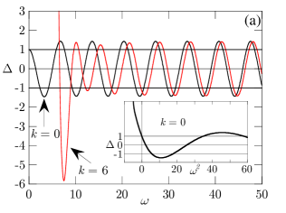
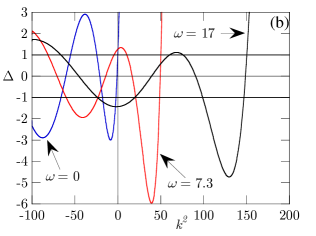
Figure 1: Generalized Lyapunov function $\Delta(\omega^{2},k^{2})$ for the profile (21): (a) $\Delta(\omega)\left(=\Delta(-\omega)\right)$ at different fixed values of $k$ (a fragment of $\Delta(\omega^{2})$ at $k=0$ for $\omega^{2}\gtrless 0$ is shown in the inset); (b) $\Delta(k^{2})$ at different fixed values $\omega$.

Since zeros of the first derivatives of $\Delta(\omega^{2},k^{2})$ cannot be points of inflection or zero-curvature by Proposition 7, we can now refine the numbering of branches $\omega_{n}(K,k)=$ $\sqrt{\omega_{n}^{2}(K,k)}$ $\left(\geq 0\right)$ in the passbands as follows:

$$0<\omega_{1}(K,k)<\omega_{2}(K,k)<\ldots\ \mathrm{if}\ K\in\mathbb{R},\ K\notin\pi\mathbb{Z};$$ (22)

$$0\leq\omega_{1}(0,k)<\omega_{2}(0,k)\leq\omega_{3}(0,k)<\omega_{4}(0,k)\leq\ldots\ \mathrm{if}\ K\in 2\pi\mathbb{Z};$$

$$0<\omega_{1}(\pi,k)\leq\omega_{2}(\pi,k)<\omega_{3}(\pi,k)\leq\omega_{4}(\pi,k)<\ldots\ \mathrm{if}\ K\in\pi+2\pi\mathbb{Z}.$$

With reference to (19) and Proposition 6, the sign of first derivatives of $\Delta(\omega^{2},k^{2})$ along $\omega_{n}(K,k)$ in the $n$th open passband $\left|\Delta\right|<1$ (see ((22₁)) is

$$\mathrm{sgn}\left[\partial\Delta/\partial(\omega^{2})\right]=-\mathrm{sgn}\left[\partial\Delta/\partial\left(k^{2}\right)\right]=\left(-1\right)^{n}.$$ (23)

The possibility of equality of two cutoffs (see (22)_2,3), i.e. of a double root of the equation $\Delta(\omega^{2})=\pm 1$, implies a zero-width stopband addressed in detail in §3.3.

For the future use, let us also mention some properties of the Dirichlet and Neumann eigenvalues $\omega_{\mathrm{D},n}^{2}$ and $\omega_{\mathrm{N},n}^{2}$ of (2) satisfying the conditions $u\left(0\right)=0,$ $u\left(1\right)=0$ and $u^{\prime}\left(0\right)=0,$ $u^{\prime}\left(1\right)=0$, respectively. It is known that $\omega_{\mathrm{D},n}\$and $\omega_{\mathrm{N},n}$ are simple zeros of the functions $M_{2}(1,0)$ and $M_{3}(1,0)$ of $\omega,$ which occur once per each stopband complemented by cutoffs (except the first stopband devoid of $\omega_{\mathrm{D},n}$). The branches $\omega_{\mathrm{D},1}(k)<~{}\omega_{\mathrm{D},2}\left(k\right)...$ and $\omega_{\mathrm{N},1}(k)<\omega_{\mathrm{N},2}(k)...$ are thus related to the passband eigenvalues $\omega_{n}\left(K,k\right)$ of (22) as

$$\omega_{\mathrm{D},2j}(k),\omega_{\mathrm{N},2j+1}(k)\in[\omega_{2j}(0,k),\omega_{2j+1}(0,k)];\ \ \omega_{\mathrm{D},2j-1}(k),\omega_{\mathrm{N},2j}(k)\in[\omega_{2j-1}(\pi,k),\omega_{2j}(\pi,k)],$$ (24)

where $j\in\mathbb{N}$ and $\omega_{\mathrm{N},1}(k)\in[0,\omega_{1}(0,k)]$. Recall that the stopbands and cutoffs are invariant with respect to the choice of the period interval $\left[y_{0},y_{0}+1\right]\equiv\left[0,1\right]$ (see Remark 1); however, the branches $\omega_{\mathrm{D},n}(k)$ and $\omega_{\mathrm{N},n}(k)$ within this area certainly depend on the choice of the point $y_{0}\equiv 0$. In other words, some fixed values $\omega,$ $k$ realize the Dirichlet or Neumann conditions at the edges of $\left[y_{0},y_{0}+1\right]$ iff $y_{0}$ is a zero of the function $M_{2}\left(y+1,y\right)\equiv im_{2}(y)$ or $M_{3}\left(y+1,y\right)\equiv im_{3}(y)$, respectively (see §3.5 for further discussion). According to (14), if $\mathbf{Q}(y)$ is an even function about the midpoint of the period $\left[y_{0},y_{0}+1\right]$ for some $y_{0}$, then the Dirichlet and Neumann branches $\omega_{\mathrm{D},n}(k)$ and $\omega_{\mathrm{N},n}(k)$ satisfying $m_{2}(y_{0})=0$ and $m_{3}(y_{0})=0$ coincide with the cutoff curves. We note the useful identity $m_{2}(y)m_{3}(y)>0$ for $\left|\Delta\right|<1$ which may be proved as follows: it obviously holds for $\Delta=0$ due to $\det\mathbf{M}=1$, and hence for any $\left|\Delta\right|<1$ due to the fact that $m_{2}(y)$ and $m_{3}(y)$ are strictly non-zero inside the passbands by (24).

3.2 WKB asymptotics of $\Delta$

Some insight into the high-frequency spectrum in the case of continuous and piecewise continuous periodicity can be gained from the WKB asymptotics [10] of the Lyapunov function $\Delta(\omega^{2},k^{2})$ at fixed $k$. To this end recall the impedance $Z=Z_{0}\sqrt{1-\mu_{2}k^{2}/\rho\omega^{2}}$ with $Z_{0}=\sqrt{\rho\mu_{1}}$ introduced in (4). For any fixed $k,$ let $\omega^{2}>k^{2}\max_{y\in\left[0,1\right]}\left(\mu_{2}/\rho\right)$ so that $Z(y)$ is real (the so-called supersonic regime). Suppose for brevity that the overall periodic profile of $Z(y)$ has at most one point of discontinuity per period. If so, the zero-order WKB approximation $\Delta_{\mathrm{WKB}}^{(0)}$ of $\Delta$ takes an especially simple form

$$\Delta_{\mathrm{WKB}}^{(0)}=\frac{1}{2}\big{(}\left[Z\right]^{1/2}+\left[Z\right]^{-1/2}\big{)}\cos\big{(}\omega\int_{0}^{1}\mu_{1}^{-1}Z\mathrm{d}y\big{)},$$ (25)

where $\pm i\omega\mu_{1}^{-1}Z$ are the eigenvalues of the matrix $\mathbf{Q}$ defined in (10)₂ and $\left[Z\right]=Z\left(y_{d}^{-}\right)/Z\left(y_{d}^{+}\right)$ with $Z\left(y_{d}^{\pm}\right)\equiv\lim_{\varepsilon\rightarrow 0}Z\left(y_{d}\pm\varepsilon\right)$ is the relative jump of $Z$ at the possible point $y_{d}$ of its periodic discontinuity. Assume first that $Z(y)$ is strictly continuous for any $y$ (not restricted to $\left[0,1\right]$) and hence $\left[Z\right]=1.$ Then Eq. (25) yields $\left|\Delta_{\mathrm{WKB}}^{(0)}\right|\leq 1$ and thus can estimate zeros of $\Delta$ but not the stopbands $\left|\Delta\right|>1,$ whose widths (the frequency gaps between cutoffs, see (19)_2,3) may well be nonzero at finite $\omega.$ Thus if $Z(y)$ is continuous then Eq. (25) merely implies that the stopband widths tend to zero at any fixed $k$ as $\omega$ tends to infinity. The latter conclusion is also valid even if $\mu_{2}/\rho$ has periodic jumps but $\rho\mu_{1}$ is continuous throughout, so that $\left[Z\right]\neq 1$ indicates existence of nonzero stopbands at finite $\omega$ but $\left[Z\right]\rightarrow\left[Z_{0}\right]=1$ at $\omega\rightarrow\infty.$ On the other hand, if $\rho\mu_{1}$ does have a jump and so $\left[Z_{0}\right]\neq 1,$ then Eq. (25) shows that the stopband widths remain nonzero as $\omega\rightarrow\infty$. Having stated this, we hasten to add that a physically sensible profile model should be related to the frequency $\omega$ in that a finite $\omega$ implies that a probing wave ”sees” appropriately abrupt variations of material properties as jumps, which are of course smoothed out by the ’infinite zoom’ of the limit $\omega\rightarrow\infty$. The above WKB conclusions on the high-frequency trends of cutoffs agree with a less general framework of, specifically, small periodic perturbations that provides expressions for the stopband widths through the Fourier series coefficients, see [3, 6].

As an example, consider again Fig. 1, which is plotted for a piecewise continuous profile (21) that gives $\left[Z\right]=12\sqrt{\left(1-4k^{2}/\omega^{2}\right)/\left(4-k^{2}/\omega^{2}\right)}$ (note that a ’single periodic discontinuity $y_{d}$’ is located at the edges of the period $T=1$ by (21); however, similarly to Remark 1, $\Delta_{\mathrm{WKB}}^{\left(0\right)}$ does not depend on the choice of the period $\left[0,1\right]$ relative to $y_{d}$). It is easy to check that the exact curves $\Delta$ shown in Fig. 1a are well fitted by the WKB approximation (25) (not displayed to avoid overloading the plot) once $\omega$ is greater enough than $k\max\sqrt{\mu_{2}/\rho}=2k$. It is also seen from Fig. 1a that increasing $\omega$ makes the curves $\Delta$ for different fixed $k$ tend to that related to $k=0,$ as predicted by Eq. (25).

In the case of two or more discontinuity points per period, applying the WKB asymptotics separately along each range of continuity modifies (25) to the form with two or more phase terms corresponding to the reflection-transmission at each discontinuity. For more examples of using the WKB approach to the periodic profile, see [23].

3.3 Zero-width stopband

3.3.1 Complementary definitions of ZWS

The following definition of a zero-width stopband (ZWS) is motivated by the possible occurrence of the second and third cases in (22).

Definition 8

If $\omega=\omega_{2n}(0,k)=\omega_{2n+1}(0,k)$ or $\omega=\omega_{2n-1}(\pi,k)=\omega_{2n}(\pi,k)$ for some $\omega,~{}k\in\mathbb{R}$ and $n\in\mathbb{N},$ then this cutoff point $\left(\omega,k\right)$ is called a ZWS.

It is essential that the cutoff curves are analytic (as any $\omega_{n}(K,k)$ with fixed $K\in\mathbb{R}$ is, see §4.1), hence if two of them meet at a point they cannot conjoin. Thus an isolated ZWS implies intersection of two cutoff curves on the $(\omega,k)$-plane and hence a saddle point $\left|\Delta\right|=1$ on the Lyapunov-function surface $\Delta(\omega^{2},k^{2}).$ For the same reason, if, exceptionally (see §3.3.3), a ZWS forms a line $\omega\left(k\right)$ of local extremum $\left|\Delta\right|=1$ of $\Delta(\omega^{2},k^{2}),$ then such line cannot have an edge point.

A comprehensive account of the properties of ZWS is based on the next proposition.

Proposition 9

The following statements are equivalent: (i) $(\omega,k)$ is a ZWS; (ii) $\Delta(\omega^{2},k^{2})=\pm 1$ and $\partial\Delta(\omega^{2},k^{2})/\partial(\omega^{2})=0$; (iii) $\Delta(\omega^{2},k^{2})=\pm 1$ and $\partial\Delta(\omega^{2},k^{2})/\partial(k^{2})=0$; (iv) $\mathbf{M}(1,0)=\pm\mathbf{I}$.

Proof. The link (i)$\Leftrightarrow$(ii) follows from Definition 8 and Proposition 7. The link (i)$\Rightarrow$(iv) can be inferred e.g. via (24), which tells us that assuming (i) entails $M_{2}(1,0)=M_{3}(1,0)=0$ and hence $M_{1}(1,0)M_{4}\left(1,0\right)=\det\mathbf{M}=1,$ where $M_{1,}$ $M_{4}$ are real by (13)₂. Since (i) also means $\mathrm{tr}\mathbf{M}\left(1,0\right)=\pm 2,$ it follows that $\mathbf{M}(1,0)=\pm\mathbf{I}$ as stated. Next let us show (iv)$\Rightarrow$(ii). Assume $\mathbf{M}(1,0)=\pm\mathbf{I}$ for some $\widetilde{\omega},\widetilde{k}\in\mathbb{R}.$ Note that $\Delta(\widetilde{\omega}^{2},\widetilde{k}^{2})=\pm 1$ by (17). The (double) eigenvalue $q=\mathrm{e}^{iK}=\pm 1$ of $\mathbf{M}(1,0)=\pm\mathbf{I}$ has geometrical multiplicity 2, hence $\widetilde{\omega}^{2}$ is an eigenvalue of $\mathcal{A}_{K}(\widetilde{k})$ of multiplicity $2$ by Corollary 3. Now consider some $K^{\prime}\in\mathbb{R}$ arbitrary close to $K$ that yields $\cos K^{\prime}=\Delta(\omega^{2},\widetilde{k}^{2})\in(-1,1).$ Since $\widetilde{\omega}^{2}$ is a double eigenvalue of $\mathcal{A}_{K}(\widetilde{k})$, the self-adjoint operator $\mathcal{A}_{K^{\prime}}(\widetilde{k})$ has two distinct simple eigenvalues $\omega^{2}\left(K^{\prime},\widetilde{k}\right)$ close to $\widetilde{\omega}^{2},$ and, by Propositions 2 and 6, these are distinct simple zeros of $\Delta(\omega^{2},\widetilde{k}^{2})-\cos K^{\prime}.$ Therefore $\Delta(\widetilde{\omega}^{2},\widetilde{k}^{2})=\pm 1$ is a local extremum of $\Delta(\omega^{2},\widetilde{k}^{2}),$ i.e. $\partial\Delta/\partial(\omega^{2})=0$ at $\widetilde{\omega}^{2},~{}\widetilde{k}^{2},$ which is equivalent to (ii). Note that reversing the above reasoning proves (ii)$\Rightarrow$(iv)  without appeal to (24), and that invoking $\mathcal{B}_{K}(\omega)$ in place of $\mathcal{A}_{K}(k)$ provides a similar proof of (iii)$\Leftrightarrow$(iv) (see also Proposition 16 below). $\blacksquare$

Note that the point $\omega=0,~{}k=0$ which yields $\Delta=1$ is not a ZWS since it does not satisfy any of the above statements, which is evident from (19)-(20).

Proposition 9 implies that the multiplicity of $\omega^{2}$, $k^{2}$ as the roots of equation $\Delta(\omega^{2},k^{2})-\cos K$ at $K\in\mathbb{R}$ is the same as their multiplicity as the eigenvalues of $\mathcal{A}_{K}(k),~{}\mathcal{B}_{K}(\omega)$ (this multiplicity is 2 at a ZWS and 1 elsewhere). This is noteworthy since such a parity does not always hold inside a ’true’ stopband $K\notin\mathbb{R},$ where a double root $\omega^{2}$ or $k^{2}$ of Eq. (18) is not a double eigenvalue of, respectively, $\mathcal{A}_{K}(k)$ or $\mathcal{B}_{K}(\omega)$ which are no longer self-adjoint for $K\notin\mathbb{R}.$ It is also pointed out that the eigenvalue $q=\mathrm{e}^{iK}$ of $\mathbf{M}(1,0)$ has an algebraic multiplicity 2 at any cutoff, while its geometrical multiplicity is 2 only at cutoffs that are ZWS.

Corollary 10

The matrix $\mathbf{M}(1,0)$ is non-semisimple for any cutoff $(\omega,k)$ unless it is a ZWS.

We note that the non-semisimple nature of the monodromy matrix at the cutoffs has important ramifications for the interpretation of its matrix logarithm, which has been proposed as the basis for dynamic effective medium models, see [25, 26].

3.3.2 Considerations of the existence of ZWS

To begin with, it is recalled that the period $T=1$ is everywhere understood as a minimal possible period, so that trivial ZWS which turn up when $T$ is a multiple of the minimal period are disregarded.

Given an arbitrary periodic $\mathbf{Q}(y),$ the condition $\mathbf{M}(1,0)=\pm\mathbf{I}$ stipulating existence of ZWS imposes three real constraints on two parameters $\omega,$ $k$ and hence is unlikely to hold. However, if the profile $\mathbf{Q}(y)$ is symmetric (even) about the midpoint of the period $\left[0,1\right]$, then, by virtue of (14), the above condition on $\mathbf{M}(1,0)$ implies only two constraints and thus such profile can be expected to yield a set of ZWS points (intersections of cutoff curves $\left|\Delta\right|=1$) on the $\left(\omega,k\right)$-plane. More precisely, since the cutoffs are independent of how the period interval is fixed (see Remark 1), ZWS are expected to exist if a given profile $\mathbf{Q}(y)$ admits such a choice of the period interval $\left[y_{0},y_{0}+1\right]\equiv\left[0,1\right]$ within which $\mathbf{Q}(y)$ is symmetric.

Note that by definition any ZWS is also an intersection of Dirichlet and Neumann branches (24) while the inverse is generally not true. Moreover, in contrast to ZWS, the Dirichlet and Neumann branches and hence their intersections $\big{\{}\omega,k\big{\}}_{\mathrm{D=N}}$ depend on the choice of the period interval. For instance, let $\mathbf{Q}(y)$ be symmetric with respect to a fixed period $\left[0,1\right].$ Then the Dirichlet and Neumann branches coincide with the cutoff curves and hence any intersection $\big{\{}\omega,k\big{\}}_{\mathrm{D=N}}$ is a ZWS (see e.g. Fig. 1 of [24]). However, if for a given $\mathbf{Q}(y)=\mathbf{Q}(y+1)$ the period is shifted so that $\mathbf{Q}(y)$ is not even about its midpoint, then a new set $\big{\{}\omega,k\big{\}}_{\mathrm{D=N}}$ includes but generally does not coincide with the (unchanged) set of ZWS.

As a simple explicit example, consider a periodically bilayered structure where $\mathbf{Q}(y)$ takes two alternating constant values within two layers $j=1,2$ that constitute a period $\left[0,1\right]$. The monodromy matrix is given by the standard expression

$$\mathbf{M}(1,0)=\left(\begin{array}[]{cc}\cos\psi_{2}\cos\psi_{1}-\frac{Z_{1}}{Z_{2}}\sin\psi_{2}\sin\psi_{1}&\frac{\mathrm{i}}{Z_{1}}\cos\psi_{2}\sin\psi_{1}+\frac{\mathrm{i}}{Z_{2}}\sin\psi_{2}\cos\psi_{1}\\ \mathrm{i}Z_{2}\cos\psi_{1}\sin\psi_{2}+\mathrm{i}Z_{1}\sin\psi_{1}\cos\psi_{2}&\cos\psi_{2}\cos\psi_{1}-\frac{Z_{2}}{Z_{1}}\sin\psi_{2}\sin\psi_{1}\end{array}\right),$$ (26)

where $Z_{j}$ is the layer impedance defined in (4) and $\psi_{j}=\omega Z_{j}d_{j}/\mu_{1j}$ with $d_{j}$ for the layer thickness. The set of Dirichlet/Neumann intersections $\big{\{}\omega,k\big{\}}_{\mathrm{D=N}}$ is defined by simultaneous vanishing of both off-diagonal components of (26), which implies the following three options: (i) $\left\{\sin\psi_{1}=0,\ \sin\psi_{2}=0\right\},$ (ii) $\left\{\cos\psi_{1}=0,\ \cos\psi_{2}=0\right\}$ and (iii) $\left\{Z_{1}=Z_{2},\ \sin\left(\psi_{1}+\psi_{2}\right)=0\right\}$, where (iii) may or may not hold for real $\omega,k$ [2]. It is seen that (i) and (iii) yield $\mathbf{M}(1,0)=\pm\mathbf{I}$. Thus (i) and maybe (iii) define ZWS, while (ii) does not.

Recall that an infinite periodically bilayered structure can always be considered over a three-layered period where the same stepwise profile $\mathbf{Q}(y)$ is symmetric. Hence the fact that any bilayered profile always admits ZWS (see e.g. Fig. 2b in §4.1) is consistent with the above conclusion that ZWS should be expected for the profiles $\mathbf{Q}(y)$ that can be defined as symmetric over some interval $\left[y_{0},y_{0}+1\right].$

3.3.3 Model examples of regular loci of ZWS

• Uniform normal impedance: $Z_{0}^{2}\equiv\rho(y)\mu_{1}(y)=const$ at any $y\in\left[0,1\right].$

Let $k=0.$ The coefficient in (4) at $k=0$ is $Z\left(\widetilde{y}\right)=Z_{0}\left(\widetilde{y}\right),$ which is constant at $Z_{0}(y)=const$ by virtue of $\mu_{1}>0.$ Alternatively, note from (10)₂ that $\mathbf{Q}(y)$ with $k=0$ and $Z_{0}=const$ has constant eigenvectors. Either of these observations readily shows that, for $k=0$, a dependence of $\omega$ on $K>0$ (not restricted to $K\in\left[0,\pi\right]$) is a straight line and thus all stopbands are ZWS, that is, there is no stopbands at all. The only difference with the case of constant $\rho$ and $\mu_{1}$ is the slope of $\omega\left(K,0\right)$ which is specified as follows:

$$\omega\left(K,0\right)=KZ_{0}/\left\langle\rho\right\rangle=K/Z_{0}\left\langle\mu_{1}^{-1}\right\rangle,$$ (27)

• Uniform speed: $c^{2}\equiv\mu_{2}(y)/\rho(y)=const$ at any $y\in\left[0,1\right]$ ($\mu_{1}(y)$ is arbitrary).

The Lyapunov function is then $\Delta(\omega^{2},k^{2})=\Delta(\omega^{2}-c^{2}k^{2},0)$, from (10)₂, and consequently

$$\omega_{n}(K,k)=\sqrt{\omega_{n}^{2}\left(K,0\right)+c^{2}k^{2}}.$$ (28)

Hence if $\omega_{n}^{2}\left(\pi m,0\right)$ with $m=0$ or $1$ is a zero-width stopband, that is, if $\omega_{n}\left(\pi m,0\right)=\omega_{n+1}\left(\pi m,0\right)$, then by (28) $\omega_{n}\left(\pi m,k\right)=\omega_{n+1}\left(\pi m,k\right)$ $\forall k,$ i.e. the entire line $\left(\omega_{n}^{2}\left(\pi m,k\right),k\right)$ for any $k\in\mathbb{R}$ is a locus of ZWS. Note from (28) and (20) that the first cutoff (which is not a ZWS) is $\omega_{1}\left(0,k\right)=ck$ $=\omega_{\mathrm{N},1}(k)$, where $\omega_{\mathrm{N},1}(k)$ is the first Neumann solution for $y\in\left[0,1\right]$.

• Uniform normal impedance and speed: $Z_{0}^{2}=const$ and $c^{2}=const$ at any $y\in\left[0,1\right].$

Now Eqs. (27) and (28) together imply that all stopbands are ZWS for any $k\in\mathbb{R}$. Note that the inverse statement is true under an additional condition of absolute continuity of $Z_{0},$ by the Borg theorem [5].

3.4 Explicit expressions for the derivatives of $\Delta$

Theorem 11

The derivatives of $\Delta(\omega^{2},k^{2})$ at any $\omega^{2},k^{2}\in\mathbb{C}\$(hence in both the passbands and the stopbands at $\omega^{2},k^{2}\in\mathbb{R}$) are given by the formula

$$\frac{\partial^{n+m}\Delta(\omega^{2},k^{2})}{\partial(\omega^{2})^{n}\partial\left(k^{2}\right)^{m}}=\frac{1}{2}{\left(-i\right)^{n}i^{m}n!m!}\int_{0}^{1}\mathrm{d}\varsigma_{1}\int_{0}^{\varsigma_{1}}\mathrm{d}\varsigma_{2}\ldots\int_{0}^{\varsigma_{n+m-1}}\mathrm{d}\varsigma_{n+m}$$ (29)

$$\qquad\times F\left(\varsigma_{1},\ldots,\varsigma_{n+m}\right)M_{2}\left(\varsigma_{n+m}+1,\varsigma_{1}\right)M_{2}\left(\varsigma_{1},\varsigma_{2}\right)\ldots M_{2}\left(\varsigma_{n+m-1},\varsigma_{n+m}\right),$$

where $M_{2}\left(y_{i},y_{j}\right)$ is a right off-diagonal component of the matricant $\mathbf{M}\left(y_{i},y_{j}\right),$ and

$$\digamma\left(\varsigma_{1},\ldots,\varsigma_{n+m}\right) \equiv\sum_{\sigma\in\Omega}f_{\sigma_{1}}\left(\varsigma_{1}\right)\ldots f_{\sigma_{n+m}}\left(\varsigma_{n+m}\right),\ f_{0}\left(\varsigma\right)\equiv\rho\left(\varsigma\right),\ f_{1}\left(\varsigma\right)\equiv\mu_{2}\left(\varsigma\right);$$ (30)

$$\Omega \equiv\left\{\left(\sigma_{1},\ldots,\sigma_{n+m}\right):\ \sigma_{i}=0,1;\ \sum\sigma_{i}=m\ \right\},$$

i.e. $\Omega$ is a set of $C_{n+m}^{n}=\left(n+m\right)!/n!m!$ permutations of a set $\left(\sigma_{1},\ldots,\sigma_{n+m}\right),$ in which each $\sigma_{i}$ is either $0$ or $1$ and their sum is $m$.

Proof. The expression (29) follows from the following property of matricants of related systems [21]: let $\mathbf{Q}(y)\mathbf{M}\left(y,y_{0}\right)=\frac{\mathrm{d}}{\mathrm{d}y}\mathbf{M}\left(y,y_{0}\right)$ and $\widetilde{\mathbf{Q}}(y)\widetilde{\mathbf{M}}\left(y,y_{0}\right)=\frac{\mathrm{d}}{\mathrm{d}y}\widetilde{\mathbf{M}}\left(y,y_{0}\right)$ where $\widetilde{\mathbf{Q}}(y)=\mathbf{Q}(y)+\mathbf{Q}_{1}(y);$ then

$$\widetilde{\mathbf{M}}\left(y,y_{0}\right) =\mathbf{M}\left(y,y_{0}\right)\widehat{\int}_{y_{0}}^{y}\left[\mathbf{I}+\mathbf{M}\left(y_{0},\varsigma\right)\mathbf{Q}_{1}\left(\varsigma\right)\mathbf{M}\left(\varsigma,y_{0}\right)\mathrm{d}\varsigma\right]$$

$$=\mathbf{M}\left(y,y_{0}\right)+\int_{y_{0}}^{y}\mathbf{M}\left(y,\varsigma_{1}\right)\mathbf{Q}_{1}\left(\varsigma_{1}\right)\mathbf{M}\left(\varsigma_{1},y_{0}\right)\mathrm{d}\varsigma_{1}+\ldots$$ (31)

$$+\int_{y_{0}}^{y}\mathrm{d}\varsigma_{1}\ldots\int_{y_{0}}^{\varsigma_{j-1}}\mathrm{d}\varsigma_{j}\mathbf{M}\left(y,\varsigma_{1}\right)\mathbf{Q}_{1}\left(\varsigma_{1}\right)\mathbf{M}\left(\varsigma_{1},\varsigma_{2}\right)\mathbf{Q}_{1}\left(\varsigma_{2}\right)\ldots\mathbf{M}\left(\varsigma_{j},y_{0}\right)+\ldots.$$

Next note that $\mathbf{Q}\left(y;\omega^{2},k^{2}\right)\equiv\mathbf{Q}\left[\omega^{2},k^{2}\right]$ defined by (10)₂ is linear in both $\omega^{2}$ and $k^{2}.$ Denote small perturbations of $\omega^{2}$ and $k^{2}$ by $\varepsilon_{\omega}$ and $\varepsilon_{k}$. From (10)₂,

$$\mathbf{Q}\left[\omega^{2}+\varepsilon_{\omega},k^{2}+\varepsilon_{k}\right]=\mathbf{Q}\left[\omega^{2},k^{2}\right]+i\left(\mu_{2}\varepsilon_{k}-\rho\varepsilon_{\omega}\right)\mathbf{\Gamma,\quad\Gamma}=\begin{pmatrix}0&0\\ 1&0\end{pmatrix}.$$ (32)

Equation (3.4) with $\mathbf{Q}_{1}\equiv i\left(\mu_{2}\varepsilon_{k}-\rho\varepsilon_{\omega}\right)\mathbf{\Gamma}$ is therefore a Taylor series of $\widetilde{\mathbf{M}}\equiv\mathbf{M}\left[\omega^{2}+\varepsilon_{\omega},k^{2}+\varepsilon_{k}\right]$ about the point $\varepsilon_{\omega}=0,$ $\varepsilon_{k}=0$, and hence the derivatives of the monodromy matrix $\mathbf{M}(1,0)$ with respect to $\omega^{2}$ and $k^{2}$ are

$$\frac{\partial^{n+m}\mathbf{M}(1,0)}{\partial(\omega^{2})^{n}\partial\left(k^{2}\right)^{m}}= \left(-i\right)^{n}i^{m}n!m!\int_{0}^{1}\mathrm{d}\varsigma_{1}\ldots\int_{0}^{\varsigma_{n+m-1}}\mathrm{d}\varsigma_{n+m}$$ (33)

$$\times F\left(\varsigma_{1},\ldots,\varsigma_{n+m}\right)\mathbf{M}\left(1,\varsigma_{1}\right)\mathbf{\Gamma M}\left(\varsigma_{1},\varsigma_{2}\right)\mathbf{\Gamma}\ldots\mathbf{M}\left(\varsigma_{n+m},0\right)$$

with $F$ defined in (30). Note that $F=\rho\left(\varsigma_{1}\right)\ldots\rho\left(\varsigma_{n}\right)$ at $m=0$ and $F=\mu_{2}\left(\varsigma_{1}\right)\ldots\mu_{2}\left(\varsigma_{m}\right)$ at $n=0.$ Equation (33) and the definition $\Delta(\omega^{2},k^{2})=\frac{1}{2}\mathrm{tr}\mathbf{M}(1,0)$ together imply

$$\frac{\partial^{n+m}\Delta(\omega^{2},k^{2})}{\partial(\omega^{2})^{n}\partial(k^{2})^{m}}=\frac{1}{2}\frac{\partial^{n+m}\mathrm{tr}\mathbf{M}(1,0)}{\partial(\omega^{2})^{n}\partial(k^{2})^{m}}=\frac{(-i)^{n}i^{m}n!m!}{2}\int_{0}^{1}\mathrm{d}\varsigma_{1}\ldots\int_{0}^{\varsigma_{n+m-1}}\mathrm{d}\varsigma_{n+m}$$ (34)

$$\qquad\times F(\varsigma_{1},\ldots,\varsigma_{n+m})\,\mathrm{tr}\big{[}\mathbf{M}(\varsigma_{n+m}+1,\varsigma_{1})\mathbf{\Gamma M}(\varsigma_{1},\varsigma_{2})\mathbf{\Gamma}\ldots\mathbf{M}(\varsigma_{n+m-1},\varsigma_{n+m})\mathbf{\Gamma}\big{]},$$

where we have used the identity $\mathrm{tr}\left[\mathbf{M}\left(1,\varsigma_{1}\right)\ldots\mathbf{M}\left(\varsigma_{n+m},0\right)\right]=\mathrm{tr}\left[\mathbf{M}\left(\varsigma_{n+m},0\right)\mathbf{M}\left(1,\varsigma_{1}\right)\ldots\right]$ and the fact that $\mathbf{M}\left(\varsigma_{n+m},0\right)=\mathbf{M}\left(\varsigma_{n+m}+1,1\right)$ due to periodicity. By definition of $\mathbf{\Gamma,}$

$$\mathbf{M\Gamma}=\begin{pmatrix}M_{2}&0\\ M_{4}&0\end{pmatrix}\quad\Rightarrow\quad\mathrm{tr}\left[\mathbf{M}^{\left(i\right)}\mathbf{\Gamma}\ldots\mathbf{M}^{(k)}\mathbf{\Gamma}\right]=M_{2}^{\left(i\right)}\ldots M_{2}^{(k)},$$ (35)

which reduces (34) to the desired form (29). $\blacksquare$

Corollary 12

The first-order derivatives of $\Delta(\omega^{2},k^{2})$ follow from (29) as

$$\frac{\partial\Delta}{\partial(\omega^{2})}=\frac{1}{2}\int_{0}^{1}\rho(y)m_{2}(y)\mathrm{d}y,\ \frac{\partial\Delta}{\partial\left(k^{2}\right)}=-\frac{1}{2}\int_{0}^{1}\mu_{2}(y)m_{2}(y)\mathrm{d}y,$$ (36)

where $im_{2}(y)=$ $M_{2}\left(y+1,y\right)$, see (15).

Interestingly, the expression (29) for any derivative of $\Delta(\omega^{2},k^{2})$ involves, apart from $\rho(y)$ and/or $\mu_{2}(y)$, only a single, right off-diagonal, element $M_{2}\left(\varsigma_{i},\varsigma_{j}\right)$ of the matricant. Recall that $\mathop{\rm Re}M_{2}=0$ by (13)₂, which conforms that (29) is real as it must be. Next we will obtain a different representation for the first derivatives of $\Delta(\omega^{2},k^{2})$ that is expressed via an eigenfunction $u(y)$ of (5). In contrast to (29), this representation is restricted to the passbands $\left|\Delta(\omega^{2},k^{2})\right|\leq 1$ and hence to $\omega^{2},k^{2}\in\mathbb{R}$. We note that the components of eigenvectors of $\mathbf{M}\left(1,0\right)$, which appear in the explicit formulas below, are understood to be referred to a basis observing the identity (13) (an obvious counterexample is the Jordan form of $\mathbf{M}(1,0)$).

Theorem 13

The first derivatives of $\Delta(\omega^{2},k^{2})$ within the open passband intervals $\Delta\in(-1,1)$ (and hence $\omega^{2},k^{2}\in\mathbb{R}$) satisfy the formulas

$$\frac{\partial\Delta}{\partial(\omega^{2})}=\frac{\sin K}{\mathbf{w}^{+}\mathbf{Tw}}\int_{0}^{1}\rho(y)\left|u(y)\right|^{2}\mathrm{d}y,\ \frac{\partial\Delta}{\partial\left(k^{2}\right)}=-\frac{\sin K}{\mathbf{w}^{+}\mathbf{Tw}}\int_{0}^{1}\mu_{2}(y)\left|u(y)\right|^{2}\mathrm{d}y,$$ (37)

where $\mathbf{w}$ is an eigenvector of $\mathbf{M}(1,0)$ corresponding to the eigenvalue $q=\mathrm{e}^{iK}$, and $u(y)$ is the first component of the vector $\mathbf{\eta}(y)=\mathbf{M}(y,0)\mathbf{w}=\left(u,i\mu_{1}u^{\prime}\right)^{\mathrm{T}}$. At the cutoffs $\Delta=\pm 1,$ Eq. (37) yields zero derivatives in the exceptional case of a ZWS, and is otherwise modified to

$$\frac{\partial\Delta}{\partial(\omega^{2})}=\frac{1}{2i\mathbf{w}_{d}^{+}\mathbf{Tw}_{g}}\int_{0}^{1}\rho(y)\left|u(y)\right|^{2}\mathrm{d}y,\ \frac{\partial\Delta}{\partial\left(k^{2}\right)}=-\frac{1}{2i\mathbf{w}_{d}^{+}\mathbf{Tw}_{g}}\int_{0}^{1}\mu_{2}(y)\left|u(y)\right|^{2}\mathrm{d}y,$$ (38)

where $\mathbf{w}_{d}$ and $\mathbf{w}_{g}$ are the proper and generalized eigenvectors of $\mathbf{M}(1,0)$ that realize its Jordan form (see (44)), and $u(y)$ is equal to the first component of the vector $\mathbf{\eta}(y)=\mathbf{M}(y,0)\mathbf{w}_{d}.$

Proof of (37). The monodromy matrix $\mathbf{M}(1,0)$ at $\left|\Delta\right|\neq 1$ has distinct eigenvalues $q\neq q^{-1}$ and hence linear independent eigenvectors $\mathbf{w}_{1},$ $\mathbf{w}_{2}$. Specify their numbering as

$$\mathbf{M}(1,0)\mathbf{w}_{1}=q\mathbf{w}_{1},~{}\mathbf{M}\left(1,0\right)\mathbf{w}_{2}=q^{-1}\mathbf{w}_{2}\mathbf{\ \ }\ \mathrm{with}\ q=\mathrm{e}^{iK}\neq q^{-1}=\mathrm{e}^{-iK}.$$ (39)

According to (3.4) and (32),

$$\frac{\partial\mathbf{M}(1,0)}{\partial(\omega^{2})} =\int_{0}^{1}\mathbf{M}(1,y)\frac{\partial\mathbf{Q}(y)}{\partial(\omega^{2})}\mathbf{M}(y,0)\mathrm{d}y=-i\mathbf{M}(1,0)\int_{0}^{1}\mathbf{P}(y)\mathrm{d}y,$$ (40)

$$\mathrm{where}\ \mathbf{P}(y) \equiv\rho(y)\mathbf{M}^{-1}(y,0)\mathbf{\Gamma M}(y,0)\ \ \big{(}\Rightarrow\mathrm{tr}\mathbf{P}(y)=\rho(y)\mathrm{tr}\mathbf{\Gamma}=0\big{)}.$$

Hence, the derivative of $\Delta=\frac{1}{2}\mathrm{tr}\mathbf{M}\left(1,0\right)$ at $\left|\Delta\right|\neq 1$ is

$$\frac{\partial\Delta}{\partial(\omega^{2})}=\frac{1}{2i}\left[q\int_{0}^{1}P_{11}(y)\mathrm{d}y+\frac{1}{q}\int_{0}^{1}P_{22}(y)\mathrm{d}y\right]=\sin KT\int_{0}^{1}P_{11}(y)\mathrm{d}y,$$ (41)

where $P_{11}$ is the upper diagonal element of $\mathbf{P}(y)$ in the base of vectors $\mathbf{w}_{1}$ and $\mathbf{w}_{2}$. For the passband case $\Delta\in(-1,1)$ being considered, the identity $\mathbf{M}^{-1}=\mathbf{TM}^{+}\mathbf{T}$ (see (13)₁) implies that

$$\mathbf{w}_{1}^{+}\mathbf{Tw}_{2}=0;\ \mathbf{w}_{1}^{+}\mathbf{Tw}_{1},\ \mathbf{w}_{2}^{+}\mathbf{Tw}_{2}\neq 0\ \ \ \ \left[(\mathbf{w}_{1}^{+}\mathbf{Tw}_{1})(\mathbf{w}_{2}^{+}\mathbf{Tw}_{2})<0\right].$$ (42)

Using (42), the equality $\mathbf{w}_{1}^{+}\mathbf{TM}^{-1}=$ $\left(\mathbf{Mw}_{1}\right)^{+}\mathbf{T}$ (following from (13)₁) and the definition of $\mathbf{\Gamma}$ given in (32), we find that

$$P_{11}(y)\Big{\rvert}_{\Delta\in(-1,1)}=\frac{\mathbf{w}_{1}^{+}\mathbf{TP}(y)\mathbf{w}_{1}}{\mathbf{w}_{1}^{+}\mathbf{Tw}_{1}}=\frac{\rho(y)\mathbf{\eta}_{1}^{+}(y)\mathbf{T\Gamma\eta}_{1}(y)}{\mathbf{w}_{1}^{+}\mathbf{Tw}_{1}}=\frac{\rho(y)\left|u(y)\right|^{2}}{\mathbf{w}_{1}^{+}\mathbf{Tw}_{1}},$$ (43)

where $\mathbf{\eta}_{1}(y)=\mathbf{M}(y,0)\mathbf{w}_{1}=\left(u,i\mu_{1}u^{\prime}\right)^{\mathrm{T}}.$ Based on the numbering in (39) it follows that $\mathbf{\eta}_{1}\left(1\right)=\mathrm{e}^{iK}\mathbf{w}_{1}$ and so $u$ is an eigenfunction of (5) (see Corollary 3). Substituting (43) into (41) and setting $\mathbf{w}_{1}$ defined in (39) as $\mathbf{w}_{1}\equiv\mathbf{w}$ leads to (37)₁. The proof of (37)₂ is the same. Note that the sign alternation (23) of both derivatives at successive cutoffs is described in (37) by the factor $\left(\mathbf{w}^{+}\mathbf{Tw}\right)^{-1}\sin K$ as follows: using $K\in\left[0,\pi\right]$ implies $\sin K\geq 0$ and alternating sign of $\mathbf{w}^{+}\mathbf{Tw}$ (due to switching between right- and leftward modes at successive cutoffs); while using unrestricted $K>0$ implies $\mathbf{w}^{+}\mathbf{Tw}<0$ (rightward mode) and alternating sign of $\sin K.$ $\blacksquare$

Proof of (38). Consider a cutoff $\Delta=\pm 1$ that is not a ZWS and hence implies a non-semisimple $\mathbf{M}(1,0).$ Denote

$$\mathbf{M}(1,0)\mathbf{w}_{d}=q_{d}\mathbf{w}_{d},\quad\mathbf{M}(1,0)\mathbf{w}_{g}=q_{d}\mathbf{w}_{g}+\mathbf{w}_{d}\quad\mathrm{at}\quad\Delta\equiv q_{d}=\pm 1,$$ (44)

which defines (not uniquely) the pair $\mathbf{w}_{d}$ and $\mathbf{w}_{g}$ as a basis in which $\mathbf{M}(1,0)$ at $\Delta=\pm 1$ has upper Jordan form. Hence

$$\frac{\partial\Delta}{\partial(\omega^{2})}=\frac{1}{2}\mathrm{tr}\frac{\partial\mathbf{M}(1,0)}{\partial\left(\omega^{2}\right)}=\frac{1}{2i}\int_{0}^{1}P_{21}(y)\mathrm{d}y,$$ (45)

where $P_{21}$ is the left off-diagonal of $\mathbf{P}(y)$ at $\Delta=\pm 1$ in the vector basis of $\mathbf{w}_{d}$ and $\mathbf{w}_{g}.$ The identity $\mathbf{M}^{-1}=\mathbf{TM}^{+}\mathbf{T}$ for a non-semisimple $\mathbf{M}(1,0)$ implies that

$$\mathbf{w}_{d}^{+}\mathbf{Tw}_{d}=0;\ \mathbf{w}_{d}^{+}\mathbf{Tw}_{g}\neq 0\ \ \ \left[\mathop{\rm Re}\mathbf{w}_{d}^{+}\mathbf{Tw}_{g}=0\ \ \mathrm{for}\ \det\mathbf{M}=1\right].$$ (46)

By (46) and the definition (40)₂ of $\mathbf{P}(y)$,

$$P_{21}(y)\Big{\rvert}_{\Delta=\pm 1}=\frac{\mathbf{w}_{d}^{+}\mathbf{TP}(y)\mathbf{w}_{d}}{\mathbf{w}_{d}^{+}\mathbf{Tw}_{g}}=\frac{\rho(y)\mathbf{\eta}_{d}^{+}(y)\mathbf{T\Gamma\eta}_{d}(y)}{\mathbf{w}_{d}^{+}\mathbf{Tw}_{g}}=\frac{\rho(y)\left|u(y)\right|^{2}}{\mathbf{w}_{d}^{+}\mathbf{Tw}_{g}},$$ (47)

where $\mathbf{\eta}_{d}(y)=\mathbf{M}(y,0)\mathbf{w}_{d}=\left(u,i\mu_{1}u^{\prime}\right)^{\mathrm{T}}.$ Inserting (47) in (45) provides (38)₁. The proof of (38)₂ is the same. $\blacksquare$

Note that (38) can also be obtained directly from (37) by taking its limit as $\left|\Delta\right|<1$ tends to $\left|\Delta\right|=\pm 1.$ To do so, proceed from (39) with $q,~{}q^{-1}$ tending to $q_{d}.$ It is always possible to choose $\mathbf{w}_{1},$ $\mathbf{w}_{2}$ so that they have $\mathbf{w}_{d}$ as a common limit and then $\left(\mathbf{w}_{1}-\mathbf{w}_{2}\right)/\left(q-q^{-1}\right)$ tends to $\mathbf{w}_{g},$ where $\mathbf{w}_{d}$ and $\mathbf{w}_{g}$ satisfy (44). By using this limiting definition of $\mathbf{w}_{g}$ and the property $\mathbf{w}_{1}^{+}\mathbf{Tw}_{2}=0$ (see (42)₁), the limit of the pre-integral factor in (37) with $\mathbf{w\equiv w}_{1}$ corresponding to $q=\mathrm{e}^{iK}$ is found to be

$$\frac{\sin K}{\mathbf{w}_{1}^{+}\mathbf{Tw}_{1}}=\frac{q-q^{-1}}{2i\mathbf{w}_{1}^{+}\mathbf{T}\left(\mathbf{w}_{1}-\mathbf{w}_{2}\right)}\underset{\Delta\rightarrow\pm 1}{\rightarrow}\frac{1}{2i\mathbf{w}_{d}^{+}\mathbf{Tw}_{g}}.$$ (48)

The factor $\mathbf{w}_{d}^{+}\mathbf{Tw}_{g}$ may also be expressed in terms of the elements $M_{i}(1,0)\equiv M_{i}$ of the matrix $\mathbf{M}(1,0)$ which satisfies (13). Using (44) yields two alternative forms of this expression as follows:

$$\mathbf{w}_{d}^{+}\mathbf{Tw}_{g}=\frac{\left|\mathbf{w}_{d}\right|^{2}M_{2}^{\ast}}{\left|M_{1}-q_{d}\right|^{2}+\left|M_{2}\right|^{2}}=\frac{\left|\mathbf{w}_{d}\right|^{2}M_{3}^{\ast}}{\left|M_{4}-q_{d}\right|^{2}+\left|M_{3}\right|^{2}}.$$ (49)

If $M_{1},~{}M_{4}\neq q_{d}$ then $M_{2},~{}M_{3}\neq 0,$ and so both formulas in (49) are equivalent, which follows from $\mathrm{tr}\mathbf{M}(1,0)=2q_{d},$ $\det\left[\mathbf{M}(1,0)-q_{d}\mathbf{I}\right]=0$ and (13)₂. If $M_{1}=q_{d}$ hence $M_{4}=q_{d}$ (or vice versa), then either $M_{2}=0$ or $M_{3}=0$, as occurs for instance if $\mathbf{Q}(y)$ is even about the midpoint of the period $\left[0,1\right]$, see the end of §3.1. Simultaneous vanishing of both $M_{2},~{}M_{3}$ is ruled out for a non-semisimple $\mathbf{M}(1,0)$.

In conclusion, the combination of results (36) and (37), (38) yields the following interesting observation.

Corollary 14

The right-hand sides of (36) are equal to those of (37) in the passbands $\Delta\in(-1,1),$ and to those of (38) at the cutoffs $\Delta=\pm 1$ (unless the cutoff is a ZWS).

3.5 Properties of the function $m_{2}(y)$

An important role of the function $m_{2}(y)$ defined in (15) is revealed by the fact that, according to (36), the first derivative of $\Delta(\omega^{2},k^{2})$ in $\omega^{2}$ or $k^{2}$ is an integral of $m_{2}(y)$ with a positive weight factor $\rho(y)$ or $\mu_{2}(y).$ Recall also that zeros of $m_{2}(y)$ are the Dirichlet solutions for the interval $\left[y,y+1\right]$, see §3.1.

Theorem 15

The continuous function $m_{2}(y)=m_{2}(y+1)$ satisfies the following properties: (i) if $\Delta(\omega^{2},k^{2})\in(-1,1)$ then $m_{2}(y)$ has no zeros for $y\in[0,1]$; (ii) if $\Delta(\omega^{2},k^{2})=\pm 1$ then $m_{2}(y)\geq 0$ for any $y\in[0,1]$ or $m_{2}(y)\leq 0$ for any $y\in[0,1]$; (iii) if $\Delta(\omega^{2},k^{2})\notin(-1,1)$ and $\omega^{2},~{}k^{2}\in\mathbb{R},$ then $m_{2}(y)$ has only finite number of zeros in $[0,1]$.

Proof. Consider (i). Suppose that $\Delta\in\left(-1,1\right)$ and there exists $\widetilde{y}$ such that $m_{2}\left(\widetilde{y}\right)=0.$ Then $\mathbf{M}\left(\widetilde{y}+1,\widetilde{y}\right)$ has eigenvalues $m_{1}\left(\widetilde{y}\right)$ and $m_{4}\left(\widetilde{y}\right)$($=m_{1}^{-1}\left(\widetilde{y}\right)$ by $\det\mathbf{M}=1$). Therefore, with reference to Remark 1, $\Delta=\frac{1}{2}\left[m_{1}\left(\widetilde{y}\right)+m_{1}^{-1}\left(\widetilde{y}\right)\right],$ where $m_{1}$ according to (15) is real (since $\omega^{2},~{}k^{2}\in\mathbb{R}$ by Lemma (5)). Hence $\left|\Delta\right|\geq 1,$ which contradicts the initial assumption. The statement (ii) follows from (i) and the analyticity of $\Delta(\omega^{2},k^{2}).$ Consider (iii). First note an identity

$$\mathbf{M}^{\prime}(y+1,y)=\mathbf{Q}(y)\mathbf{M}(y+1,y)-\mathbf{M}(y+1,y)\mathbf{Q}(y)\ \Rightarrow\ m_{2}^{\prime}(y)=\frac{m_{1}(y)-m_{4}(y)}{\mu_{1}(y)},$$ (50)

where ${}^{\prime}\equiv\mathrm{d}/\mathrm{d}y$ (if $y$ is a point discontinuity of a piecewise continuous $\mathbf{Q}(y),$ then $\mathrm{d/d}y$ is a right or left derivative). Since $\mu_{1}(y)>0$, it follows that $m_{2}^{\prime}(y)=0$ iff $m_{4}(y)=m_{1}(y).$ Now let us suppose the inverse of (iii), i.e., that $\Delta\notin(-1,1)$ admits the existence of an infinite set $\{y_{n}\}_{1}^{\infty}$ for which $m_{2}(y_{n})=0$. Without loss of generality we may assume that $\lim_{n\rightarrow\infty}y_{n}=y_{0}\in[0,1]$. Then $m_{2}(y_{0})=0$ and $m_{2}^{\prime}\left(y_{0}\right)=0$. As shown above, $m_{2}(y_{0})=0$ yields $m_{4}\left(y_{0}\right)=m_{1}^{-1}\left(y_{0}\right)$ and so we have $\Delta\notin(-1,1)$ for $\Delta=\frac{1}{2}\left[m_{1}(y_{0})+m_{1}^{-1}(y_{0})\right]\notin(-1,1)$ where $m_{1}$ is real due to $\omega^{2},~{}k^{2}\in\mathbb{R}.$ It therefore follows that $m_{4}\left(y_{0}\right)=m_{1}^{-1}\left(y_{0}\right)\neq m_{1}\left(y_{0}\right).$ According to (50), this contradicts $m_{2}^{\prime}\left(y_{0}\right)=0.$ $\blacksquare$

The above result together with Eq. (36) provides a simple criterion for a ZWS, which complements Proposition 9.

Proposition 16

The following statements are equivalent: (i) $(\omega,k)$ is a ZWS; (ii) $m_{2}(y)=0$ for any $y.$

Proof. Assume (i). Then ${\mathbf{M}}(1,0)=\pm{\mathbf{I}}$ by Proposition 9. Hence by (16) ${\mathbf{M}}(y+1,y)=\pm{\mathbf{I}}$ and so $m_{2}\equiv 0,$ which is (ii). Now assume (ii). It requires that $\Delta=\pm 1$ by Theorem 15 and yields $\partial\Delta/\partial(\omega^{2})=0$ by Eq. (36)₁. According to Proposition 9, $\Delta(\omega^{2},k^{2})=\pm 1,$ $\partial\Delta(\omega^{2},k^{2})/\partial(\omega^{2})=0$ implies that $(\omega,k)$ is a ZWS, which is (i). $\blacksquare$

Interestingly, the function $m_{3}(y),$ whose zeros are the Neumann solutions for the interval $\left[y,y+1\right]$, shares some, but not all, of the properties of $m_{2}(y).$ For instance, $m_{3}(y)$ displays the same properties (i), (ii) stated by Theorem 15 for $m_{2}(y)$ but it does not have the property (iii). The dissimilarity stems from the fact that (50)₁ yields $m_{3}^{\prime}(y)=\left(\mu_{2}k^{2}-\rho\omega^{2}\right)\left(m_{1}-m_{4}\right),$ where, in contrast to (50)₁, the first factor is not sign-definite. Also the derivatives of $\Delta(\omega^{2},k^{2})$ are not expressible via $m_{3}(y)$ as they are via $m_{2}(y)$ in (36). As a result, Proposition 16 does not hold for $m_{3}(y)$ in the sense that while it is true that $m_{3}(y)=0$ for any $y$ if $(\omega,k)$ is a ZWS, the inverse statement is not. An immediate counter-example is the point $\omega=0,~{}k=0,$ where $m_{3}(y)=0$ for any $y$ by (20) but this point is not a ZWS; moreover, the model case $\mu_{2}(y)/\rho(y)=const\equiv c^{2}$ mentioned in §3.3 ensures $m_{3}\equiv 0$ on the whole cutoff line $\omega_{1}\left(0,k\right)=ck$ (see (28)) which has no ZWS points. Thus, the Dirichlet solution $\omega_{\mathrm{D},n}(k)$ for $\left[y,y+1\right]$ does not depend on $y$ only if $(\omega_{\mathrm{D},n},k)$ is a zero-width stopband, but the same is not generally true for the Neumann solutions.

4 The dispersion surface $\omega_{n}(K,k)$

In this Section, we address the multisheet surface $\omega_{n}\left(K,k\right)=\sqrt{\omega_{n}^{2}(K,k)}\left(\geq 0\right)$ which is defined by Eq. (18), and study the curves in its cuts taken at constant $K$, constant $k$ and constant $\omega$.

Remark 17

If Eq. (18) with either $K$ or $k$ or $\omega$ being fixed defines a differentiable function, then its derivative of any order can be expressed in terms of partial derivatives of $\Delta(\omega^{2},k^{2})$ given in (29).

Below we examine in detail the first non-zero derivatives. The higher-order ones are easy to obtain in a similar fashion by differentiating (18). It is understood hereafter that $\omega,~{}k\in\mathbb{R}.$ By (18), $\omega_{n}(K,k)=\omega_{n}\left(-K,k\right)=\omega_{n}\left(K,-k\right)$ which permits confining considerations to $\mathop{\rm Re}K\geqslant 0,~{}k\geqslant 0.$

4.1 The function $\omega_{n}(k)$ for fixed $K$

Consider the dependence of $\omega_{n}(k)\equiv\omega_{n}(K,k)$ for fixed $K$, Fig. 2. By Eq. (18), the branches $\omega_{n}(k)$ are defined as level curves $\Delta(\omega^{2},k^{2})\left(=\cos K\right)=const,$ which lie in the passbands for fixed $K\in\mathbb{R}\Leftrightarrow$ $\left|\Delta\right|\leq 1$ and in the stopbands for fixed complex $K\in\pi\mathbb{Z}+i\left(\mathbb{R}\backslash 0\right)\Leftrightarrow\left|\Delta\right|>1$ (note that the branch numbering (22) does not apply in the stopbands, see the discussion of Fig. 2 below).

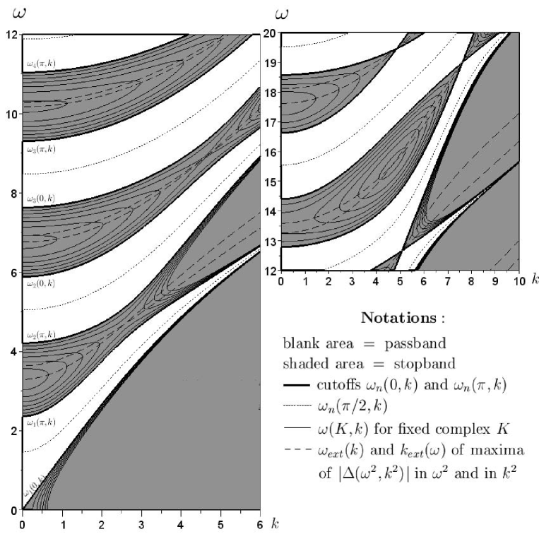
Figure 2: (a) (left) The curves $\omega_{n}(k)\equiv\omega_{n}(K,k)$ at different fixed $K$ for the profile (21). (b) Sections of the curves for the piecewise constant profile defined by $\mu_{1}=~{}\mu_{2}=1,$ $\rho=1$ for $y\in[0,1/2)$ and $\mu_{1}=\mu_{2}=12,$ $\rho=2$ for $y\in(1/2,1]$.

Proposition 18

If $\omega\neq 0$ and $\partial\Delta/\partial(\omega^{2})\neq 0,$ then

$$\frac{\mathrm{d}\omega_{n}}{\mathrm{d}k}=\frac{k}{\omega_{n}}\frac{\mathrm{d}\omega_{n}^{2}}{\mathrm{d}\left(k^{2}\right)}=-\frac{k}{\omega_{n}}\frac{\partial\Delta/\partial\left(k^{2}\right)}{\partial\Delta/\partial(\omega^{2})},$$ (51)

where by (36), (37) and (38)

$$\frac{\mathrm{d}\omega_{n}^{2}}{\mathrm{d}\left(k^{2}\right)}=\frac{\int_{0}^{1}\mu_{2}(y)m_{2}(y)\mathrm{d}y}{\int_{0}^{1}\rho(y)m_{2}(y)\mathrm{d}y}\Bigg{\rvert}_{\begin{subarray}{c}K\in\mathbb{R}\ \mathrm{or}\\ K\in\pi\mathbb{Z}+i\mathbb{R}\end{subarray}}=\frac{\int_{0}^{1}\mu_{2}(y)\left|u_{n}(y)\right|^{2}\mathrm{d}y}{\int_{0}^{1}\rho(y)\left|u_{n}(y)\right|^{2}\mathrm{d}y}\Bigg{\rvert}_{K\in\mathbb{R}}.$$ (52)

In addition,

$$\frac{\mathrm{d}\omega_{1}}{\mathrm{d}k}\Big{\rvert}_{\begin{subarray}{c}\omega=0\\ k=0\end{subarray}}=\sqrt{\frac{\left\langle\mu_{2}\right\rangle}{\left\langle\rho\right\rangle}};\qquad\frac{\mathrm{d}\omega_{n}}{\mathrm{d}k}\Big{\rvert}_{\begin{subarray}{c}\omega\neq 0\\ k=0\end{subarray}}=0,\qquad\frac{\mathrm{d}k}{\mathrm{d}\omega_{1}}\Big{\rvert}_{\begin{subarray}{c}\omega=0\\ k\neq 0\end{subarray}}=0.$$ (53)

The former equality follows from (19) or else from (52) where $m_{2}(y)$ and $u_{1}(y)$ are constant at $\omega,\ k=0$ in view of (20). The two other equalities in (53) follow from (51) and $\mathrm{d}\omega_{n}^{2}/\mathrm{d}\left(k^{2}\right)\neq 0$ (note that $\omega=0,\ k\neq 0$ belongs to the stopband area where (52)₁ applies, see Fig. 2a).

For $K\in\mathbb{R},$ the excluded case $\partial\Delta/\partial(\omega^{2})=0$ in (51) is related to ZWS discussed in §3.3. According to Proposition 9, if $\partial\Delta/\partial(\omega^{2})$ at $K\in\mathbb{R}$ becomes zero then so does $\partial\Delta/\partial\left(k^{2}\right)$ and their simultaneous vanishing implies a ZWS. Barring extraordinary cases mentioned in 3.3.3, ZWS is an intersection point $\left(\omega,k\right)_{\mathrm{zws}}$ of two analytic curves $\omega_{n}\left(k\right)$ (as rigorously confirmed in Proposition 19 below), so there exist two derivatives at $\left(\omega,k\right)_{\mathrm{zws}}$. Their values can be determined by continuity from either of equations (52) applied in the vicinity of $\left(\omega,k\right)_{\mathrm{zws}}.$ Note that Eq. (52)₁ is not defined strictly at $\left(\omega,k\right)_{\mathrm{zws}}$ (where $m_{2}(y)=0$ $\forall y$, see Proposition 16) while Eq. (52)₂ is, provided that $u_{n}(y)$ implies two different eigenfunctions from a subspace corresponding to two intersecting curves $\omega_{n}\left(k\right)$ at $\left(\omega,k\right)_{\mathrm{zws}}$.

Proposition 19

The curves $\omega_{n}(k)$ for fixed $K\in\mathbb{R}$ are monotonically increasing at $k>0$.

Proof. The function $\omega_{n}^{2}(k^{2})$ is analytic for any $K\in\mathbb{R}$ since $\mathcal{A}_{K}(k)$ is a family of analytic operators of Kato’s type A [12]. Hence if $\partial\omega_{n}^{2}/\partial(k^{2})=0$ for some real $k^{2},$ then there exists complex $\widetilde{k}^{2}$ in the vicinity of $k^{2}$ for which $\omega^{2}=\omega_{n}^{2}\big{(}\widetilde{k}^{2}\big{)}$ is real. But this would mean that the operator $\mathcal{B}_{K}(\omega)$ has a complex eigenvalue $k^{2}$ equal to $\widetilde{k}^{2},$ which is impossible. Thus $\omega_{n}(k)$ at $K\in\mathbb{R}$ is a monotonic function. It increases by virtue of (52)₂. To provide a fully self-consistent proof within the operator approach, note that (52)₂ can also be obtained by applying the perturbation theory [15] to $\mathcal{A}_{K}$ given by (6), so that

$$\frac{\mathrm{d}\omega_{n}^{2}}{\mathrm{d}(k^{2})}=\frac{\mathrm{d}~{}~{}}{\mathrm{d}(k^{2})}\frac{\left(\mathcal{A}_{K}u_{n},u_{n}\right)_{\rho}}{\left\|u_{n}\right\|_{\rho}^{2}}=\frac{1}{\left\|u_{n}\right\|_{\rho}^{2}}\big{(}\frac{\mathrm{d}\mathcal{A}_{K}}{\mathrm{d}(k^{2})}u_{n},u_{n}\big{)}_{\rho}=\frac{\int_{0}^{1}\mu_{2}(y)\left|u_{n}(y)\right|^{2}\mathrm{d}y}{\int_{0}^{1}\rho(y)\left|u_{n}(y)\right|^{2}\mathrm{d}y}.\ \ \blacksquare$$ (54)

Consider the example plotted in Fig. 2. It demonstrates monotonicity of the curves $\omega_{n}(k)\equiv\omega_{n}(K,k)$ at fixed $K\in\mathbb{R}$ by tracing the cutoff curves at $K=0,\pi$ ($\Leftrightarrow\left|\Delta\right|=1$) and the curves at $K=\pi/2$ ($\Leftrightarrow\Delta=0$) within the passbands. Figure 2 also shows that, by contrast, the curves $\omega\left(k\right)\equiv\omega(K,k)$ in the stopbands, i.e. at fixed complex $K\in\pi\mathbb{Z}+i\left(\mathbb{R}\backslash 0\right)$ ($\Leftrightarrow$ the level curves $\left|\Delta\right|=const>1$), may be not monotonic and can take a looped shape, either semi-closed or even fully closed. Note that the numbering of such curves cannot be defined by the rule (22) restricted to the passbands. A looped shape is due to a vertical tangent at a point where $\partial\Delta/\partial(\omega^{2})=0$ (see (51), (52)₁). In any stopband except the lowest one, there exists a pair of curves $\omega_{\mathrm{ext}}(k)$ and $k_{\mathrm{ext}}(\omega),$ on which $\left|\Delta(\omega^{2},k^{2})\right|=\cosh\left(\mathop{\rm Im}K\right)$ has maxima in $\omega^{2}$ and in $k^{2}$ (in $k$ at $k\neq 0$), respectively. Hence each stopband except the lowest must contain looped curves $\omega\left(k\right)$ with a vertical tangent as they cross the curve $\omega_{\mathrm{ext}}(k)$ - unless the latter fully merges with $k_{\mathrm{ext}}(\omega)$ as in the model case $\mu_{2}(y)/\rho(y)=const$ mentioned in §3.3. The curves $\omega_{\mathrm{ext}}(k)$ and $k_{\mathrm{ext}}\left(\omega\right)$ may intersect within a given stopband thus indicating a saddle point or an absolute extremum of $\Delta(\omega^{2},k^{2})$ (the latter is exemplified in Fig. 2b, see the family of closed level curves $\left|\Delta\right|>1$). At the same time, $\omega_{\mathrm{ext}}(k)$ and $k_{\mathrm{ext}}(\omega)$ cannot contact the cutoff curves except at the point of a ZWS (see Fig. 2b), which is always a saddle point of $\Delta(\omega^{2},k^{2})$.

It is shown in Appendix A3 that the lower bound for the branches $\omega_{n}(k)$ at $K\in\mathbb{R}$ is $\min_{y\in\left[0,1\right]}\sqrt{\mu_{2}/\rho}.$ In the remainder of this subsection we prove that this bound is also a common limit of $\omega_{n}(k).$ To do so, it is convenient to introduce the velocity $v_{n}=\omega_{n}/k.$ First we specify the derivative of $v_{n}(k)$ in order to demonstrate its monotonicity (note that it is easy to similarly obtain sign-definite derivatives at fixed $K\in\mathbb{R}$ for any other optional choice of the pair of spectral parameters among $\omega,~{}k~{}$and $v$ or $s=v^{-1}$).

Lemma 20

Let $K\in\mathbb{R}$, $n\in\mathbb{\mathbb{N}}$ be fixed. Then $v_{n}^{2}(k^{2})\equiv\omega_{n}^{2}\left(k^{2}\right)/k^{2}$ is a decreasing function with derivative

$$\frac{\mathrm{d}v_{n}^{2}}{\mathrm{d}(k^{2})}=-\frac{1}{k^{4}}\frac{\int_{0}^{1}\mu_{1}|u_{n}^{\prime}(y)|^{2}\mathrm{d}y}{\int_{0}^{1}\rho|u_{n}(y)|^{2}\mathrm{d}y}<0,$$ (55)

where $u_{n}$ and $u_{n}^{\prime}$ are defined by $\mathbf{\eta}(y)\equiv\left(u,~{}i\mu_{1}u^{\prime}\right)^{\mathrm{T}}=\mathbf{M}(y,0)\mathbf{w}$ taken at $\omega_{n}^{2}$ (cf. (37)).

Proof. Multiply Eq. (2) by $u$ $(=u_{n})$, integrate by parts and divide the result by $k^{2}$, to yield

$$v_{n}^{2}\int_{0}^{1}\rho|u_{n}(y)|^{2}\mathrm{d}y=\frac{1}{k^{2}}\int_{0}^{1}\mu_{1}|u_{n}^{\prime}|^{2}\mathrm{d}y+\int_{0}^{1}\mu_{2}|u_{n}|^{2}\mathrm{d}y.$$ (56)

Substituting from (56) along with (54) into $\mathrm{d}\omega_{n}^{2}/\mathrm{d}(k^{2})=k^{2}\mathrm{d}v_{n}^{2}/\mathrm{d}(k^{2})+v_{n}^{2}$ leads to (55). The same result follows by applying the perturbation theory [15] similarly as in (54), whence $\mathrm{d}v_{n}^{2}/\mathrm{d}(k^{2})=-((\mu_{1}u_{n}^{\prime})^{\prime},u_{n})_{\rho}/k^{4}\left\|u_{n}\right\|_{\rho}^{2}$ and integrating by parts yields (55). $\blacksquare$

Proposition 21

Let $K\in\mathbb{R}$ be fixed. Then for any $n\in\mathbb{\mathbb{N}}$

$$\lim_{k\rightarrow\infty}\frac{\omega_{n}^{2}}{k^{2}}=\min_{y\in\left[0,1\right]}\frac{\mu_{2}(y)}{\rho(y)}.$$ (57)

Proof. Rewrite (2) in the form

$$-(\mu_{1}u^{\prime})^{\prime}+k^{2}\left(\frac{\mu_{2}}{\rho}-\frac{\omega^{2}}{k^{2}}\right)\rho u=0.$$ (58)

where $v^{2}=\omega^{2}/k^{2}$. For any fixed $v\equiv\alpha>\min\sqrt{\mu_{2}/\rho},$ the coefficient $\left(\mu_{2}/\rho\right)-v^{2}$ changes sign on the interval $[0,1]$ and hence there exist infinitely many distinct values $k^{2}>0$ which satisfy (58) (see more in [9]). The latter means that any curve $v_{n}(k),$ $n\in\mathbb{\mathbb{N}},$ intersects the line $\alpha(k)\equiv\alpha$ for any $\alpha>\min\sqrt{\mu_{2}/\rho}.$ Combining this statement with the above-mentioned facts that all $v_{n}(k)$ are decreasing and have the lower bound $\min\sqrt{\mu_{2}/\rho}$ yields (57). $\blacksquare$

It is noteworthy that there is no common limit for a finite spectrum of eigenvalues of a discrete Schrödinger operator with a large potential [14].

Figure 3: The Floquet branches $\omega_{n}(K)\equiv\omega_{n}(K,k)$ at fixed $k=1.$ (b) Real isofrequency branches $K_{j}(k)$ at fixed $\omega=8$. The same profile (21) is used. The cutoff values of $\omega$ in (a) and of $k$ in (b) can be compared with Figs. 1 and 2a.

4.2 Function $\omega_{n}(K)$ for fixed $k$

Consider the function $\omega_{n}(K)\equiv\omega_{n}\left(K,k\right)$ implicitly defined by Eq. (18): $\Delta(\omega^{2},k^{2})=\cos K$ at fixed $k$. Since $\omega_{n}(k)$ is periodic and even, it suffices to deal with one-half of the Brillouin zone $\mathop{\rm Re}K\in\left[0,\pi\right]$, see Fig. 3a. For brevity, denote the cutoff values $\omega_{n}\left(\pi m,k\right)$ of $\omega_{n}\left(K,k\right)$ as

$$\omega_{n}\left(\pi m,k\right)\equiv\omega_{n,m},\ \ \ m=0,1.$$ (59)

Let us indicate the passbands and stopbands of $\omega_{n}(K,k)$ by $\mathop{\rm Im}K=0$ and $\mathop{\rm Im}K\neq 0$, respectively (the latter being short for $K=\pi m+i\mathop{\rm Im}K\neq\pi m$). Explicit expressions for the first non-zero derivative of $\omega_{n}(K)$ readily follow by expanding both sides of (18) and invoking the formulas for $\partial\Delta/\partial(\omega^{2})$ obtained in §3.4. Note that Eq. (60) with (37)₁ for real $K$ (see below) can also be obtained by means of perturbation theory [15] applied to an appropriately modified form of (2), (3) with an operator explicitly dependent upon $K$.

Proposition 22

If either (i) $\mathop{\rm Im}K=0$ and $K\neq\pi m$ (hence $\partial\Delta/\omega\neq 0$ by Proposition 6) or (ii) $\mathop{\rm Im}K\neq 0$ and $\partial\Delta/\partial\omega\neq 0,$ then

$$\frac{\mathrm{d}\omega_{n}}{\mathrm{d}K}=-\frac{\sin K}{\left(\partial\Delta/\partial\omega\right)_{\omega_{n}}},$$ (60)

where $\sin K=\sqrt{1-\Delta^{2}}$ and$\ \partial\Delta/\partial\omega=2\omega\partial\Delta/\partial(\omega^{2})$ is given by (36₁) or (37)₁ for (i) and by (36)₁ for (ii). If $K=\pi m$ and $\partial\Delta/\partial\omega\neq 0,$ then

$$\frac{\mathrm{d}\omega_{n}}{\mathrm{d}K}=0,\quad\frac{\mathrm{d}^{2}\omega_{n}}{\mathrm{d}K^{2}}=\frac{\left(-1\right)^{m+1}}{\left(\partial\Delta/\partial\omega\right)_{\omega_{n,m}}},\$$ (61)

where $\omega_{n,m}=\omega_{n,m}(k)$ are the roots of equation $\Delta(\omega^{2},k^{2})=\left(-1\right)^{m}$ and $\partial\Delta/\partial\omega$ is given by (36)₁ or (38)₁.

Consider the special cases where $\partial\Delta/\partial\omega=0$. Let $K=\pi m$ and $\partial\Delta/\partial\omega=0$ at $\omega\neq 0,$ which implies a cutoff $\omega_{n,m}$ corresponding to a ZWS. Then

$$\frac{\mathrm{d}\omega_{n}}{\mathrm{d}K}={\left(-1\right)^{m+n+1}}\big{/}\sqrt{\left(-1\right)^{m+1}\left(\partial^{2}\Delta/\partial\omega^{2}\right)_{\omega_{n,m}}}.$$ (62)

Next let $\mathop{\rm Im}K\neq 0$ and $\partial\Delta/\partial\omega=0,$ which defines the point $\omega\equiv\omega_{\mathrm{ext}}$ in a stopband at which $\left|\Delta(\omega)\right|=\cosh\left(\mathop{\rm Im}K\right)$ reaches its maximum $\left|\Delta_{\mathrm{ext}}\right|>1$ (see Fig. 2 and its discussion in §4.1). The function $\mathop{\rm Im}K(\omega)$ satisfies $\left(\mathrm{d}\mathop{\rm Im}K/\mathrm{d}\omega\right)_{\omega_{\mathrm{ext}}}=0$ and

$$\frac{\mathrm{d}^{2}\mathop{\rm Im}K}{\mathrm{d}\omega^{2}}=(-1)^{m}\,\frac{\left(\partial^{2}\Delta/\partial\omega^{2}\right)_{\omega_{\mathrm{ext}}}}{\sqrt{\Delta_{\mathrm{ext}}^{2}-1}}\quad\left(<0\ \mathrm{for}\mathop{\rm Im}K>0\right).$$ (63)

The explicit form of $\partial^{2}\Delta/\partial\omega^{2}$, which appears in (62), (63) and is negative at $m=0$ and positive at $m=1$, is defined by (29). It can be written in the following equivalent forms

$$\frac{\partial^{2}\Delta}{\partial\omega^{2}} =4\omega^{2}\frac{\partial^{2}\Delta}{\partial(\omega^{2})^{2}}=-4\omega^{2}\int_{0}^{1}\mathrm{d}y\int_{0}^{y}\rho(y)\rho\left(y_{1}\right)M_{2}(y_{1}+1,y)M_{2}\left(y,y_{1}\right)\mathrm{d}y_{1}$$

$$=-2\omega^{2}\int_{0}^{1}\mathrm{d}y\int_{y}^{y+1}\rho(y)\rho\left(y_{1}\right)M_{2}\left(y+1,y_{1}\right)M_{2}(y_{1},y)\mathrm{d}y_{1}$$ (64)

$$=-2\omega^{2}\int_{0}^{1}\mathrm{d}y\int_{0}^{1}\rho(y)\rho\left(y+y_{1}\right)M_{2}\left(y+1,y+y_{1}\right)M_{2}(y+y_{1},y)\mathrm{d}y_{1},$$

where $\partial\Delta/\partial\omega=0$ and $\omega\neq 0$ (i.e. $\partial\Delta/\partial(\omega^{2})=0$) have been used. Finally, consider the case $\omega=0,$ which implies $\partial\Delta/\partial\omega=0,\ \partial^{2}\Delta/\partial\omega^{2}=2\partial\Delta/\partial(\omega^{2})$. If both $\omega=0$ and $k=0$ ($\Rightarrow K=0$), then referring to (19), the derivative (62) for $m=1$ reduces to

$$\frac{\mathrm{d}\omega_{1}}{\mathrm{d}K}=1\big{/}\sqrt{\left\langle\rho\right\rangle\left\langle\mu_{1}^{-1}\right\rangle}.\$$ (65)

If $\omega=0$ and $k>0$ ($\Rightarrow K=i\mathop{\rm Im}K\neq 0$), then $\left(\mathrm{d}\mathop{\rm Im}K/\mathrm{d}\omega\right)_{\omega=0}=0$ and (63) becomes

$$\frac{\mathrm{d}^{2}\mathop{\rm Im}K}{\mathrm{d}\omega^{2}}=\frac{2\left[\partial\Delta/\partial(\omega^{2})\right]_{\omega=0}}{\sqrt{\Delta^{2}\left(0,k^{2}\right)-1}},$$ (66)

where $\left[\partial\Delta/\partial(\omega^{2})\right]_{\omega=0}<0$ is given by (36)₁.

It is evident from Eq. (60) that the Floquet branches $\omega_{n}(K)$ for any fixed real $k$ are monotonic in $K\in\left[0,\pi\right]$. For completeness, let us also mention two important results from the general theory of Schrödinger equation [15, 19, 11] that extend to the case of Eq. (2) with fixed $k.$ These results state that $\mathop{\rm Im}K(\omega)$ is a convex function and that each branch $\omega_{n}(K)$ has one and only one inflection point in $K\in\left[0,\pi\right]$, unless it is the lowest branch $\omega_{1}(K)$ at $k=0$ or a branch bounded by a ZWS at either or both cutoffs $K=\pi m,$ in which case there is no inflection points. Note in conclusion that Eqs. (61) and (62) provide an explicit definition for the near-cutoff asymptotics of branches $\omega_{n}(K)$ that were analyzed in [7] by a different means (the scaling approach, also extended in [7] to 2D-periodicity).

4.3 The function $K(k)$ for fixed $\omega$

Consider the dependence of $K(k)=\arccos\Delta(\omega^{2},k^{2})$ on $k\geq 0$ at fixed $\omega.$ Let the branches $K_{j}(k)\in\left[0,\pi\right]$ for real $K$ be numbered in the order of increasing $k.$ Since $\omega_{n}\left(k\right)\equiv\omega_{n}(K,k)$ is strictly increasing in $k$ (see Fig. 2), the number of real branches $K_{j}(k)$ at any fixed value $\omega$ is fully defined by its position with respect to the frequency-cutoff points at $k=0$: there is a single real branch $K_{1}(k)$ for a fixed $\omega$ in the interval $0<\omega<\omega_{2}\left(\pi,0\right);$ two real branches $K_{1}(k),$ $K_{2}(k)$ for $\omega$ in $\omega_{2}\left(\pi,0\right)<\omega<\omega_{3}\left(0,0\right)$ … etc. Besides, the first real branch $K_{1}\left(k\right)$ starts at $k=0$ and spans a range $[0,\pi)$ or $(0,\pi]$ iff $\left|\Delta(\omega^{2},0)\right|<1,$ i.e. iff the given $\omega$ is fixed within the passband at $k=0.$ For example, the value $\omega=8\in\left(\omega_{3}(0,0),\omega_{4}(\pi,0)\right)$ in Fig. 2 yields three real branches $K_{j}(k)$ with $K_{1}(k)\in[0,\pi),$ see Fig. 3b.

Denote by

$$k_{j,m}(\omega)\equiv k_{j,m},\ \ \ m=0,1,$$ (67)

the roots of equation $\Delta(\omega^{2},k^{2})=\left(-1\right)^{m}$ which define the points at which $K_{j}(k)=\pi m$ and the given $\omega$ is the cutoff; these points $k_{j,m}$ are separated by the stopband intervals $\left|\Delta\right|>1$ where $\mathop{\rm Im}K\neq 0.$ The explicit form of the first derivative of $K\left(k\right)$ for real or complex $K$ follows from (18) and the formulas for $\partial\Delta/\partial(k^{2})$ in exactly the same way as that $\omega_{n}(k)$ in §4.2.

Proposition 23

If $K\neq\pi m$ and $k\neq 0,\$then

$$\frac{\mathrm{d}K}{\mathrm{d}k}=-\frac{\partial\Delta/\partial k}{\sin K},$$ (68)

where $\partial\Delta/\partial k\neq 0$ for real $K.$ If $K_{j}\left(k\right)=\pi m$ at $k\neq 0$ and $\left(\partial\Delta/\partial k\right)_{k_{j,m}}\neq 0,\$then the locally defined inverse function $k\left(K\right)$ satisfies

$$\frac{\mathrm{d}k}{\mathrm{d}K_{j}}=0,\quad\frac{\mathrm{d}^{2}k}{\mathrm{d}K_{j}^{2}}=\frac{\left(-1\right)^{m+1}}{\left(\partial\Delta/\partial k\right)_{k_{j,m}}}.$$ (69)

If $k=0,$ then

$$\frac{\mathrm{d}K_{1}}{\mathrm{d}k}=\begin{cases}0,\quad\frac{\mathrm{d}^{2}K_{1}}{\mathrm{d}k^{2}}=-\frac{2}{\sin K_{1}}\left[\partial\Delta/\partial(k^{2})\right]_{k=0}&\mathrm{at}\ K_{1}\neq\pi m,\\ \sqrt{2\left(-1\right)^{m+1}\left[\partial\Delta/\partial\left(k^{2}\right)\right]_{k=0}}&\mathrm{at}\ K_{1}=\pi m.\end{cases}$$ (70)

Consider the implication of possibly existing ZWS. Assume that a fixed $\omega$ is a ZWS for some $k\neq 0.$ This means that $K_{j}\left(k_{j,m}\right)=\pi m$ and $\left(\partial\Delta/\partial k\right)_{k_{j,m}}=0$ where $k_{j,m}\neq 0.$ Then (69) is altered to

$$\frac{\mathrm{d}K_{j}}{\mathrm{d}k}=\left(-1\right)^{m+j}\sqrt{\left(-1\right)^{m+1}\left(\partial^{2}\Delta/\partial k^{2}\right)_{k_{j,m}}}.$$ (71)

Now assume that a fixed $\omega$ is a ZWS at $k=0$, i.e. let $K_{1}=\pi m$ and $\left[\partial\Delta/\partial(k^{2})\right]_{k=0}=0.$ Then $\mathrm{d}K_{1}/\mathrm{d}k=0$ by (70), and

$$\frac{\mathrm{d}^{2}K_{1}}{\mathrm{d}k^{2}}=\sqrt{2\left(-1\right)^{m+1}\left[\partial^{2}\Delta/\partial(k^{2})^{2}\right]_{k=0}}.$$ (72)

The second-order derivative of $\Delta$ in (71), (72) can be obtained by differentiating (36)₂ in the same way as in (4.2). Note that $\partial^{2}\Delta/\partial(k^{2})^{2}$ also appears in the formula analogous to (63) for $\mathrm{d}^{2}\mathop{\rm Im}K/\mathrm{d}k^{2}$ at the point $k_{\mathrm{ext}}$ where $\mathrm{d}\mathop{\rm Im}K/\mathrm{d}k=0$.

Thus, by (69) and (71), all real branches $K_{j}(k)$ at fixed $\omega$ have vertical tangents at the edge points $K_{j}\left(k_{j,m}\right)=\pi m,~{}k_{j,m}\neq 0$ (see Fig. 1b), unless the cutoff $\omega=\omega_{n}\left(\pi m,k_{j,m}\right)$ is a ZWS in which case $K_{j}(k)$ does not make a right angle with the line $K=\pi m.$ In turn, by (70) and (72), the real branch $K_{1}(k)$ has a horizontal tangent at $k=0,~{}K\neq\pi$ and a non-zero first derivative at $k=0,$ $K=\pi$, unless $\omega=\omega_{n}\left(\pi,0\right)$ is a ZWS stopband in which case the slope of $K_{1}(k)$ vanishes at $k=0,$ $K=\pi$.

Remark 24

If the cutoff $\omega=\omega_{n}\left(\pi,0\right)$ is not a ZWS, then (i) the curve $K_{1}(k)=K_{1}\left(-k\right)$ has a kink at $k=0$; (ii) $\mathbf{\nabla}\omega(K,k)=\mathbf{0}$ at $k=0$ by virtue of (53) and (61).

4.4 Convexity of the closed isofrequency branch $K_{1}\left(k\right)$

The normal to real isofrequency branches $K_{j}(k)$ defines the direction of group velocity $\mathbf{\nabla}\omega(K,k)$ which makes their shape relevant to many physical applications. In particular, negative curvature of an isofrequency curve is known to give rise to rich physical phenomena related to wave-energy focussing. Since the function $K(k)=\arccos\Delta$ with $\left|\Delta\right|\leq 1$ defines a unique $K\in\left[0,\pi\right],$ no vertical line can cross twice the curve $K(k);$ however, this by itself does certainly not preclude a negative curvature. In fact any real branch $K_{j}(k),$ which extends from $K_{j}=0$ to $K_{j}=\pi,$ has vertical tangents at those edge points and hence must have at least one inflection between them (unless the exceptional case of ZWS, see §4.3). This simple argument, however, does not apply to the first branch $K_{1}(k)$ if the reference $\omega$ is taken within the passband range at $k=0$ and hence $K_{1}(k)$ does not reach one of the edge points $0$ or $\pi.$ In other words, the situation in question is when $K_{1}(k)$ extended by symmetry to any real $K,~{}k\lessgtr 0$ forms a closed curve.

In the present subsection we address an important case of a relatively low frequency $\omega$ which is restricted to the passband below the first cutoff $\omega_{1}\left(\pi,0\right)$ at the edge of the Brillouin zone $K=\pi$ at $k=0.$ For any fixed $\omega<\omega_{1}\left(\pi,0\right)$, there is a single real isofrequency branch $K_{1}(k)=\arccos\Delta(\omega^{2},k^{2})\in\left[0,\pi\right)$ that is continuous in the definition domain $k\in\left[-k_{1,0},k_{1,0}\right],$ where $k_{1,0}$ is the least root of equation $\Delta=1$ (see (67)). According to (91)₁,

$$\omega\sqrt{\left\langle\rho\right\rangle/\left\langle\mu_{2}\right\rangle}\leq k_{1,0}(\omega)\leq\omega\max\nolimits_{y\in\left[0,1\right]}\sqrt{\rho(y)/\mu_{2}(y)}.$$ (73)

We will show that $K_{1}(k)$ is strictly convex. The proof is preceded by a lemma.

Lemma 25

For fixed $\omega<\omega_{1}\left(\pi,0\right),$ derivatives of the function $\Delta(\omega^{2},k^{2})$ of any order in $k^{2}$ are strictly positive at $k^{2}\geq 0$.

Proof. Let $\omega=0.$ Then $\Delta(0,k^{2})>0$ for $k^{2}\geq 0$ by (84) and so $\partial\Delta(0,k^{2})/\partial(k^{2})>0$ for $k^{2}\geq 0$ because $\Delta(k^{2})$ at fixed $\omega^{2}$ satisfies the conditions of the Laguerre theorem (see Proposition 7). In other words, all zeros of $\partial\Delta(0,k^{2})/\partial(k^{2})$ lie in $k^{2}<0$ (see Fig. 1b). Now let $0<\omega<\omega_{1}\left(\pi,0\right).$ This means that $-1<\Delta(\omega^{2},0)<1$ and so the first zero of $\partial\Delta(\omega^{2},k^{2})/\partial(k^{2}),$ which is where $\Delta\leq-1,$ still lies in $k^{2}<0.$ Thus, if $\omega<\omega_{1}\left(\pi,0\right)$ then $\partial\Delta(\omega^{2},k^{2})/\partial(k^{2})>0$ for $k^{2}\geq 0$ and hence, again by the Laguerre theorem, $\partial^{p}\Delta/\partial(k^{2})^{p}>0$ for $k^{2}\geq 0$ and for any $p\geq 1.$ $\blacksquare$

Theorem 26

The curve $K_{1}(k)$ is convex at any fixed $\omega$ such that $\omega<\omega_{1}\left(\pi,0\right).$

Proof. The second derivative of $K_{1}(k)$ is

$$K_{1}^{\prime\prime}(k)=-\left(1-\Delta^{2}\right)^{-3/2}h,~{}\quad h(k)\equiv\Delta\Big{(}\frac{\partial\Delta}{\partial k}\Big{)}^{2}+\left(1-\Delta^{2}\right)\frac{\partial^{2}\Delta}{\partial k^{2}},$$ (74)

where $-1<\Delta^{2}<1$ for $k\in\left(-k_{1,0},k_{1,0}\right)$, see (67). Note that $\partial\Delta/\partial k=0$ at $k=0$. Let $\omega<\omega_{1}\left(\pi,0\right)$. Then $h(0)=\left(1-\Delta^{2}\right)\partial^{2}\Delta/\partial k^{2}>0$ and $h^{\prime}(k)=\left(\partial\Delta/\partial k\right)^{3}+\left(1-\Delta^{2}\right)\partial^{3}\Delta/\partial k^{3}>0$ according to Lemma 25. Due to $h(0)>0$ and $h^{\prime}\left(k\right)>0$ at $k>0,$ it follows that $h(k)>0$ at $k>0.$ Hence $K_{1}^{\prime\prime}(k)<0$ in its definition domain $\left[-k_{1,0},k_{1,0}\right]$. Thus, $K_{1}(k)$ is convex. $\blacksquare$

The obtained result sets an important benchmark against any artefacts of approximate analytical and/or numerical modelling of the first isofrequency curve $K_{1}(k)=\arccos\Delta,$ which are possible as a result of truncating series for $\arccos$ or for $\Delta=\frac{1}{2}\mathrm{tr}\mathbf{M}(1,0)$ (see (12)). Figure 4 demonstrates an example where an approximate computation of $K_{1}(k)$ produces a spurious concavity. In this regard we note that Figure 1 of [20], which is sketch of the generic relation between $K$ and $k$ for fixed but small $\omega$, incorrectly gives the suggestion that concavities can occur.

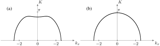
Figure 4: (a) The approximate and (b) the exact first isofrequency curve $K_{1}(k)=\arccos\left[\frac{1}{2}\mathrm{tr}\mathbf{M}(1,0)\right]$ at fixed $\omega\left(=3.4\right)<\omega_{1}\left(\pi,0\right)$ for a periodically piecewise constant profile defined by $\mu_{1}=1,~{}\mu_{2}=0.35,$ $\rho=0.2$ at $y\in[0,1/2)$ and $\mu_{1}=0.95,~{}\mu_{2}=0.4,$ $\rho=0.19$ at $y\in(1/2,1].$ The monodromy matrix (12), which in this case is $\mathbf{M}\left(1,0\right)=\left(\exp\mathbf{Q}_{2}\right)\left(\exp\mathbf{Q}_{1}\right)$ with $\mathbf{Q}_{j}$ defined by (10)₂, is computed via the series of the co-factor exponentials, keeping four terms for each of them in the case (a) and 30 terms in the case (b).

In conclusion, a remark is in order concerning the high-frequency case where the first isofrequency branch $K_{1}(k)$ defined in $k\in\left[-k_{1,0},k_{1,0}\right]$ is accompanied by the higher-order branches $K_{j\geq 2}(k).$ In general, $K_{1}(k)$ should stay convex and $K_{j\geq 2}(k)$ should have not more than a single inflection point. However, it seems possible to construct a theoretical example, though quite peculiar, of a periodic profile, for which the above is not true.

Acknowledgements

The authors thank Prof. E. Korotyaev for helpful discussions. AKK acknowledges support from the University Bordeaux 1 (project AP-2011).

Appendix

A1. Properties of the operators $\mathcal{A}_{K}$ and $\mathcal{B}_{K}$

It is evident that the operator $\mathcal{A}_{K}$ defined in (6) is symmetric for $k^{2},~{}K\in\mathbb{R}$, i.e.

$$\left(\mathcal{A}_{K}u,v\right)_{\rho} =-\int_{0}^{1}\left(\mu_{1}u^{\prime}\right)^{\prime}v^{\ast}\mathrm{d}y+k^{2}\int_{0}^{1}\mu_{2}uv^{\ast}\mathrm{d}y=\int_{0}^{1}\mu_{1}u^{\prime}v^{\prime\ast}\mathrm{d}y+k^{2}\int_{0}^{1}\mu_{2}uv^{\ast}\mathrm{d}y$$

$$=-\int_{0}^{1}\left(\mu_{1}v^{\prime}\right)^{\prime\ast}u\mathrm{d}y+k^{2}\int_{0}^{1}\mu_{2}uv^{\ast}\mathrm{d}y=\left(u,\mathcal{A}_{K}v\right)_{\rho},$$ (75)

using the identities $\mu_{1}u^{\prime}v^{\ast}\mid_{0}^{1}=\mu_{1}v^{\prime}u^{\ast}\mid_{0}^{1}=0$ which follow from the boundary condition (7) on $u,v\in D_{K}$ iff $K$ is real. The proof of the symmetry of $\mathcal{B}_{K}$ for $\omega^{2},~{}K\in\mathbb{R}$ is the same.

We now demonstrate that $\mathcal{A}_{K}$ and $\mathcal{B}_{K}$ are self-adjoint with discrete spectra $\sigma\left(\mathcal{A}_{K}\right)=\left\{\omega_{n}^{2}\right\}_{1}^{\infty}$ and $\sigma\left(\mathcal{B}_{K}\right)=\left\{k_{n}^{2}\right\}_{1}^{\infty}$ corresponding to complete sets of eigenfunctions (as stated in §2). This is achieved by explicit construction of the resolvent of each operator, $\mathcal{R}_{K,\lambda}=\left(\mathcal{A}_{K}-\omega^{2}\right)^{-1}$ or $\mathcal{R}_{K,\lambda}=\left(\mathcal{B}_{K}-k^{2}\right)^{-1}$, where $\lambda$ implies $\omega^{2}$ or $k^{2}.$ In order to do so consider the equivalent equations

$$\begin{array}[]{c}\left(\mathcal{A}_{K}-\omega^{2}\right)u=g,\ \ \omega^{2}\notin\sigma\left(\mathcal{A}_{K}\right)\\ \left(\mathcal{B}_{K}-k^{2}\right)u=g,\ \ k^{2}\notin\sigma\left(\mathcal{B}_{K}\right)\end{array}\ \ \mathrm{with}\ u(y)\in D_{K},\ g(y)\in L_{\rho,\mu_{2}}^{2}\left[0,1\right],$$ (76)

which can be recast as

$$\mathbf{\eta}^{\prime}(y)-\mathbf{Q}(y)\mathbf{\eta}(y)=\mathbf{\gamma}(y)\ \mathrm{with}\ \mathbf{\gamma}(y)=\begin{pmatrix}0\\ if(y)\end{pmatrix},\ \mathbf{\eta}\left(1\right)=\mathrm{e}^{iK}\mathbf{\eta}(0),$$ (77)

where $f=-i\rho g$ for $\mathcal{A}_{K}$, $f=i\mu_{2}g$ for $\mathcal{B}_{K}$, and $\mathbf{\eta}$, $\mathbf{Q}$ are defined in (7), (10), respectively. The solution to (77) is a superposition of its partial solution $\mathbf{\eta}_{p}$ with the solution $\mathbf{\eta}_{0}(y)$ of the corresponding homogeneous equation:

$$\mathbf{\eta}(y)=\mathbf{\eta}_{p}(y)+\mathbf{\eta}_{0}(y),\ \mathbf{\eta}_{p}(y)=\int_{0}^{y}\mathbf{M}\left(y,\varsigma\right)\mathbf{\gamma}\left(\varsigma\right)\mathrm{d}\varsigma,\ \mathbf{\eta}_{0}(y)=\mathbf{M}(y,0)\mathbf{\eta}_{0}(0)\mathbf{.}$$ (78)

The vector $\mathbf{\eta}_{0}(0)$ is found from the quasi-periodic boundary condition that yields $\mathbf{\eta}_{p}\left(1\right)+\mathbf{\eta}_{0}\left(1\right)=\mathrm{e}^{iK}\mathbf{\eta}_{0}(0).$ Thus

$$\mathbf{\eta}(y) =\int_{0}^{1}\mathbf{G}\left(y,\varsigma\right)\mathbf{\gamma}\left(\varsigma\right)\mathrm{d}\varsigma\ \ \mathrm{with}$$ (79)

$$\mathbf{G}\left(y,\varsigma\right) =\mathbf{M}\left(y,\varsigma\right)H\left(y-\varsigma\right)-\mathbf{M}(y,0)\left[\mathbf{M}(1,0)-\mathrm{e}^{iK}\mathbf{I}\right]^{-1}\mathbf{M}\left(1,\varsigma\right),$$

where $H\left(y-\varsigma\right)$ is the Heaviside function and $\mathrm{e}^{iK}$ is not an eigenvalue of $\mathbf{M}(1,0)$ for the given $\omega^{2}\notin\sigma\left(\mathcal{A}_{K}\right)$, $k^{2}\notin\sigma\left(\mathcal{B}_{K}\right)$. It can be checked that the Green-function tensor $\mathbf{G}\left(y,\varsigma\right)$ satisfies the identity $\mathbf{G}\left(y,\varsigma\right)=-\mathbf{TG}^{+}(\varsigma,y)\mathbf{T}$, so that its right off-diagonal component satisfies $G_{12}\left(y,\varsigma\right)=-G_{12}^{\ast}\left(y,\varsigma\right)$. By (79)₁,

$$u=\mathcal{R}_{K,\lambda}g=\int_{0}^{1}G\left(y,\varsigma;\lambda\right)f\left(\varsigma\right)\mathrm{d}\varsigma,\mathrm{\ where}\ G\left(y,\varsigma;\lambda\right)=iG_{12}\left(y,\varsigma\right).$$ (80)

It is seen that the resolvent $\mathcal{R}_{K,\lambda}$ is an integral (bounded) self-adjoint operator generated by a piecewise continuous kernel. The symmetry $\left(\mathcal{R}_{K,\lambda}g,v\right)=\left(g,\mathcal{R}_{K,\lambda}v\right)$ follows for any $v\in D_{K}$ from $G\left(y,\varsigma;\lambda\right)=G^{\ast}\left(\varsigma,y;\lambda\right)$ or else from the symmetry of $\mathcal{A}_{K},\ \mathcal{B}_{K}$. Thus $\mathcal{R}_{K,\lambda}$ satisfies the Hilbert-Schmidt theorem and $\mathcal{A}_{K},$ $\mathcal{B}_{K}$ therefore possess the above-mentioned properties.

A2. Bounds of the function $\Delta(\omega^{2},k^{2})$

The far-reaching properties of the analytic function $\Delta(\omega^{2},k^{2})$ stated in Proposition 7 follow by applying Laguerre’s theorem to $\Delta(\omega^{2})$ at any fixed $k^{2}$ and to $\Delta(k^{2})$ at any fixed $\omega^{2}$. A function satisfying Laguerre’s theorem must be an entire function of order of growth less than 2. Verification of this condition for $\Delta(\omega^{2},k^{2})$ requires its uniform estimation in $\mathbb{C}$. The WKB asymptotic expansion (see §3.2) is not well-suited for the task in hand. Here we derive explicit bounds which show that $\Delta(\omega^{2})$ and $\Delta(k^{2})$ for, respectively, any $k^{2}$ and $\omega^{2}$ are entire functions of order of growth $\frac{1}{2}$. The derivation consists of two Lemmas in which the following auxiliary notation is used: $f_{\max}\equiv\max f(y),~{}f_{\min}\equiv\min f(y)$ for $f(y)=\rho(y),~{}\mu_{1,2}(y)$ and $y\in\left[0,1\right]$.

Lemma 27

For any $\omega,~{}k\in\mathbb{C},$

$$\left|\Delta(\omega^{2},k^{2})\right|\leq\cosh\sqrt{\mu_{1\min}^{-1}\big{(}{\mu_{2\max}\left|k\right|^{2}+\rho_{\max}\left|\omega\right|^{2}}\big{)}}.$$ (81)

Proof. For any 2$\times$2 matrix $\mathbf{A}$ with the entries $\left(a_{1}..a_{4}\right),$ define $\left|\mathbf{A}\right|$ as

$$\left|\mathbf{A}\right|=\begin{pmatrix}\left|a_{1}\right|&\left|a_{2}\right|\\ \left|a_{3}\right|&\left|a_{4}\right|\end{pmatrix}$$ (82)

and note that $\left|\prod\nolimits_{n}\mathbf{A}_{n}\right|\leq\prod\nolimits_{n}\left|\mathbf{A}_{n}\right|$ where the entrywise inequality is understood. Recall that $\widehat{\int}$ appearing in (12) implies a product integral and is an exponential when the integrand matrix is constant. Hence it follows from (10)₂, (12) and (17) that

$$\begin{array}[]{c}\left|\Delta(\omega^{2},k^{2})\right|=\frac{1}{2}\left|\mathrm{tr}\widehat{\int}_{0}^{1}\left[\mathbf{I}+\mathbf{Q}(y)\mathrm{d}y\right]\right|=\frac{1}{2}\left|\mathrm{tr}\widehat{\int}_{0}^{1}\left[\mathbf{I}+i\begin{pmatrix}0&-\mu_{1}^{-1}(y)\\ \mu_{2}(y)k^{2}-\rho(y)\omega^{2}&0\end{pmatrix}\mathrm{d}y\right]\right|\\ \leq\frac{1}{2}\mathrm{tr}\widehat{\int}_{0}^{1}\left[\mathbf{I}+i\begin{pmatrix}0&\mu_{1\min}^{-1}\\ \mu_{2\max}\left|k\right|^{2}+\rho_{\max}\left|\omega\right|^{2}&0\end{pmatrix}\mathrm{d}y\right]=\cosh\sqrt{\frac{\mu_{2\max}\left|k\right|^{2}+\rho_{\max}\left|\omega\right|^{2}}{\mu_{1\min}}}\ \blacksquare.\end{array}$$ (83)

The inequality (83) confirms that $\Delta(\omega^{2})$ and $\Delta(k^{2})$ are entire functions with order of growth not greater than $\frac{1}{2}$ in each argument. Next we demonstrate that $\Delta$ for certain $\omega^{2},~{}k^{2}$ grows no slower than an exponential of power $\frac{1}{2}$ of $\omega^{2}$ and/or $k^{2}$. This will enable us to conclude that the order of growth of $\Delta(\omega^{2})$ and $\Delta(k^{2})$ is precisely $\frac{1}{2}$.

Lemma 28

For $\omega^{2},~{}k^{2}\in\mathbb{R},$

$$\left|\Delta(\omega^{2},k^{2})\right|\geq\cosh\sqrt{\mu_{1\max}^{-1}\big{(}{\mu_{2\min}k^{2}-\rho_{\max}\omega^{2}}\big{)}}\ \mathrm{for}\ k^{2}\geq\mu_{2\min}^{-1}{\rho_{\max}}\omega^{2}.$$ (84)

Proof. First introduce a class $\mathcal{M}$ of 2$\times$2 matrices such that

$$\mathcal{M}=\left\{\begin{pmatrix}a_{1}&-ia_{2}\\ ia_{3}&a_{4}\end{pmatrix}\right\},\ a_{j}\geq 0,\ j=1..4.$$ (85)

For two matrices $\mathbf{A}$ and $\mathbf{B}$ from $\mathcal{M}$, we say that $\mathbf{A\geq}_{\mathcal{M}}~{}\mathbf{B}$ iff $a_{j}\geq b_{j}$ for any $j=1..4$. If $\mathbf{A}\in\mathcal{M}$ and $\mathbf{B}\in\mathcal{M}$ then $\mathbf{AB}\in\mathcal{M}$ also. Therefore, if $\mathbf{A}_{k},\ \mathbf{B}_{k}\in\mathcal{M}$ and $\mathbf{A}_{k}\geq_{\mathcal{M}}~{}\mathbf{B}_{k}$ for any $k=1..n$ then $\mathbf{A}_{1}..\mathbf{A}_{n}\geq_{\mathcal{M}}\mathbf{B}_{1}..\mathbf{B}_{n}$ and $\mathrm{tr}\left(\mathbf{A}_{1}..\mathbf{A}_{n}\right)\geq\mathrm{tr}\left(\mathbf{B}_{1}..\mathbf{B}_{n}\right)$ (which is easy to check for $n=2$ and is therefore valid for any $n$). We note from (10)₂ that $\mu_{2\min}k^{2}\geq\rho_{\max}\omega^{2}$ implies $\mathbf{I}+\mathbf{Q}(y)\mathrm{d}y\in\mathcal{M}$ for any $y\in\left[0,1\right]$ and $\mathrm{d}y>0;$ moreover,

$$\mathbf{I}+\mathbf{Q}(y)\mathrm{d}y\geq_{\mathcal{M}}~{}\mathbf{I}+i\begin{pmatrix}0&-\mu_{1\max}^{-1}\\ \mu_{2\min}k^{2}-\rho_{\max}\omega^{2}&0\end{pmatrix}\mathrm{d}y$$ (86)

and consequently

$$\Delta(\omega^{2},k^{2}) =\frac{1}{2}\mathrm{tr}\widehat{\int}_{0}^{1}\left[\mathbf{I}+\mathbf{Q}(y)\mathrm{d}y\right]\geq\frac{1}{2}\mathrm{tr}\widehat{\int}_{0}^{1}\left[\mathbf{I}+i\begin{pmatrix}0&-\mu_{1\max}^{-1}\\ \mu_{2\min}k^{2}-\rho_{\max}\omega^{2}&0\end{pmatrix}\mathrm{d}y\right]$$

$$=\cosh\sqrt{\frac{\mu_{2\min}k^{2}-\rho_{\max}\omega^{2}}{\mu_{1\max}}}.\ \ \qquad\blacksquare$$ (87)

A3. Bounds of the first eigenvalue $\omega_{1}^{2}(K,k)$

Proposition 29

For $K\in[-\pi,\pi]$ and $k\in\mathbb{R}$, the first eigenvalue $\omega_{1}^{2}(K,k)$ is bounded as follows

$$k^{2}\min_{y\in\left[0,1\right]}\frac{\mu_{2}(y)}{\rho(y)}\leq\omega_{1}^{2}(K,k)\leq\frac{\left\langle\mu_{1}\right\rangle}{\left\langle\rho\right\rangle}K^{2}+\frac{\left\langle\mu_{2}\right\rangle}{\left\langle\rho\right\rangle}k^{2}.$$ (88)

Proof. Let $u_{1}\in D_{K}$ with the unit norm $\left\|u_{1}\right\|_{\rho}=1$ be the eigenfunction vector of $\mathcal{A}_{K}$ corresponding to the eigenvalue $\omega_{1}^{2}$. Then

$$\omega_{1}^{2}=\left(\mathcal{A}_{K}u_{1},u_{1}\right)_{\rho}=\int_{0}^{1}\mu_{1}\left|u_{1}^{\prime}\right|^{2}\mathrm{d}y+k^{2}\int_{0}^{1}\mu_{2}\left|u_{1}\right|^{2}\mathrm{d}y\geq k^{2}\int_{0}^{1}\frac{\mu_{2}}{\rho}\rho\left|u_{1}\right|^{2}\mathrm{d}y\geq k^{2}\min_{y\in\left[0,1\right]}\frac{\mu_{2}}{\rho}.$$ (89)

An equivalent proof of the lower bound (89) follows by noting that the initial equation (2) yields zero as the sum of the positive operator $-\left(\mu_{1}u^{\prime}\right)^{\prime}$ and the operator multiplying $u$ by $\left(k^{2}\mu_{2}-\omega^{2}\rho\right),$ implying that the latter factor must be negative. In order to obtain the upper bound, introduce the function $v(y)=\left\langle\rho\right\rangle\mathrm{e}^{iKy}$ such that $v(y)\in D_{K}$ and $\left\|v\right\|_{\rho}=1$. Hence $\omega_{1}^{2}$ as a minimal eigenvalue of $\mathcal{A}_{K}$ satisfies

$$\omega_{1}^{2}=\inf_{u\in D_{K},\ \left\|u\right\|_{\rho}=1}\left(\mathcal{A}_{K}u_{1},u_{1}\right)_{\rho}\leq\left(\mathcal{A}_{K}v,v\right)_{\rho}=\frac{\left\langle\mu_{1}\right\rangle}{\left\langle\rho\right\rangle}K^{2}+\frac{\left\langle\mu_{2}\right\rangle}{\left\langle\rho\right\rangle}k^{2}.\ \blacksquare$$ (90)

Corollary 30

The bounds of the first cutoff at the centre and the edge of the Brillouin zone are, respectively,

$$k\min_{y\in\left[0,1\right]}\sqrt{\frac{\mu_{2}(y)}{\rho(y)}}\leq\omega_{1}\left(0,k\right)\leq k\sqrt{\frac{\left\langle\mu_{2}\right\rangle}{\left\langle\rho\right\rangle}};\quad\omega_{1}\left(0,k\right)<\omega_{1}\left(\pi,k\right)\leq\sqrt{\frac{\left\langle\mu_{1}\right\rangle}{\left\langle\rho\right\rangle}\pi^{2}+\frac{\left\langle\mu_{2}\right\rangle}{\left\langle\rho\right\rangle}k^{2}}.$$ (91)

As stated in Proposition 21, the lower bound (88) of $\omega_{1}(K,k)$ and hence of all curves $\omega_{n}\left(K,k\right)$ for $K\in\mathbb{R}$ is also their limit at $k\rightarrow\infty$. Note that $\omega_{1}\left(0,k\right)\geq\omega_{\mathrm{N},1}(k)$ by (24), where $\omega_{\mathrm{N},1}(k)$ is the lowest branch of solutions of the Neumann problem for $y\in\left[0,1\right]$. It has the same bounds and the same limit at $k\rightarrow\infty$ as $\omega_{1}\left(0,k\right)$. In this regard, recall the model example $\mu_{2}(y)/\rho(y)=const\equiv c^{2}$ (see §3.2), where $\omega_{1}\left(0,k\right)=\omega_{\mathrm{N},1}(k)=ck$ merge together with their upper and lower bounds. By (91)₁, unless $\omega_{1}\left(0,k\right)$ is a straight line, it has an inflection point (and so does $\omega_{\mathrm{N},1}(k)$). Furthermore, the case of constant $\rho,~{}\mu_{1,2}$ is an elementary example of the equality of the upper bound in (88) and (91)₂.

References

- [1] Allaire, G., and Orive, R. On the band gap structure of Hill’s equation. J. Math. Anal. Appl. 306 (2005), 462–480.
- [2] Al’shits, V. I., Deschamps, M., and Lyubimov, V. N. Dispersion anomalies of shear horizontal guided waves in two- and three-layered plates. J. Acoust. Soc. Am. 118 (2005), 2850–2859.
- [3] Auld, B. A. Acoustic Fields and Waves in Solids, Vol. I. Wiley Interscience, New York, 1973.
- [4] Binding, P., and Volkmer, H. Eigencurves for two-parameter Sturm-Liouville equations. SIAM Rev. 38 (1996), 27–48.
- [5] Borg, G. Uniqueness theorems in the spectral theory of . In Proc. 11th Scandinavian Congress of Mathematicians (1952), Johan Grundt Tanums Forlag, Oslo, pp. 276–287.
- [6] Brillouin, L. Wave Propagation in Periodic Structures. Dover, New York, 1953.
- [7] Craster, R. V., Kaplunov, J., and Pichugin, A. V. High-frequency homogenization for periodic media. Proc. R. Soc. A 466 (2010), 2341–2362.
- [8] Gatignol, P., Potel, C., and de Belleval, J.-F. Two families of modal waves for periodic structures with two field functions: a Cayleigh-Hamilton approach. Acta Acust. Acust 93 (2007), 959–975.
- [9] Glazman, I. Direct Methods of Qualitative Spectral Analysis of Singular Differential Operators. Fizmatgiz, Moscow (in Russian), 1963.
- [10] Heading, J. An Introduction to Phase Integral Methods. Wiley-Methuen, New York, 1962.
- [11] Kargaev, P., and Korotyaev, E. Effective masses and conformal mappings. Comm. Math. Phys. 169 (1995), 597–625.
- [12] Kato, T. Perturbation Theory For Linear Operators. Springer Verlag, Berlin, 1995.
- [13] Korotyaev, E. Inverse problem and the trace formula for the Hill operator, II. Math. Z. 231 (1999), 345–368.
- [14] Korotyaev, E., and Kutsenko, A. A. Inverse problem for the discrete 1D Schrödinger operator with small periodic potentials. Comm. Math. Phys. 261 (2006), 673–692. Inverse problem for the discrete 1D Schrödinger operator with large periodic potentials, in press.
- [15] Krein, M. The fundamental propositions of the theory of -zones of stability of a canonical system of linear differential equations with periodic coefficients. In In Memory of A. A. Andronov (Moscow, 1955), Izd. Akad. Nauk SSSR, pp. 413–498.
- [16] Kuchment, P. Floquet Theory for Partial Differential Equations. Birkhäuser Verlag, Basel, 1993.
- [17] Magnus, W., and Winkler, S. Hill’s Equation. Interscience, New York, 1966.
- [18] Marchenko, V. A. Sturm-Liouville Operators and their Applications. Birkhauser, Basel, 1986.
- [19] Marchenko, V. A., and Ostrovskii, I. V. Approximation of periodic potentials by finite-zone potentials. Selecta Math. Sovietica 6 (1987), 101–136.
- [20] Norris, A. N., and Santosa, F. Shear wave propagation in a periodically layered medium - an asymptotic theory. Wave Motion 16 (1992), 35–55.
- [21] Pease, M. C. Methods of Matrix Algebra. Academic Press, New York, 1965.
- [22] Reed, M., and Simon, B. Methods of Modern Mathematical Physics. IV. Analysis of Operators. Academic Press, New York, 1978.
- [23] Shuvalov, A., Poncelet, O., and Golkin, S. V. Existence and spectral properties of shear horizontal surface acoustic waves in vertically periodic half-spaces. Proc. R. Soc. A 465 (2009), 1489–1511.
- [24] Shuvalov, A., Poncelet, O., and Kiselev, A. Shear horizontal waves in transversely inhomogeneous plates. Wave Motion 45 (2008), 605–615. Note the misprints: replace by in two lines above (2), interchange and in the 2nd line of (18) and invert the units of in the plots.
- [25] Shuvalov, A. L., Kutsenko, A. A., and Norris, A. N. Divergence of the logarithm of a unimodular monodromy matrix near the edges of the Brillouin zone. Wave Motion 47 (2010), 370–382.
- [26] Shuvalov, A. L., Kutsenko, A. A., Norris, A. N., and Poncelet, O. Effective Willis constitutive equations for periodically stratified anisotropic elastic media. Proc. R. Soc. A 467 (2011), 1749–1769.
- [27] Titchmarsh, E. The Theory of Functions. Oxford University Press, 1976.