On the effective shear speed in 2D phononic crystals

Abstract

The quasistatic limit of the antiplane shear-wave speed (’effective speed’) $c$ in 2D periodic lattices is studied. Two new closed-form estimates of $c$ are derived by employing two different analytical approaches. The first proceeds from a standard background of the plane wave expansion (PWE). The second is a new approach, which resides in $\mathbf{x}$-space and centers on the monodromy matrix (MM) introduced in the 2D case as the multiplicative integral, taken in one coordinate, of a matrix with components being the operators with respect to the other coordinate. On the numerical side, an efficient PWE-based scheme for computing $c$ is proposed and implemented. The analytical and numerical findings are applied to several examples of 2D square lattices with two and three high-contrast components, for which the new PWE and MM estimates are compared with the numerical data and with some known approximations. It is demonstrated that the PWE estimate is most efficient in the case of densely packed stiff inclusions, especially when they form a symmetric lattice, while in general it is the MM estimate that provides the best overall fitting accuracy.

I Introduction

Effective material properties of composites have been and remain a topic of much interest in micromechanics, see the reviews BM ; MMP ; PA . The recent surge of research into the properties of metamaterials and phononic crystals has heightened attention, particularly for periodic systems. In this context, considerable work has been done on the low-frequency, or quasistatic, limit of the antiplane shear-wave speed in 2D periodic structures (referred to as the ’effective speed’ $c$ in the following; note that this value also yields the limit of the fundamental velocity branch of shear plate waves). A natural tool for tackling the problems with periodicity is the plane-wave expansion (PWE). An explicit PWE-expression of the effective speed $c$ via an infinite sum of Fourier coefficients has been obtained in KAG and was broadly used afterwards for computing $c$ in various periodic materials. Note some other semi-analytical techniques that were used for numerical evaluation of $c,$ such as scaling ABDW and mixed-variational NWSA methods. In turn, the multiple-scattering theory (MST), which deals directly with the inclusion/matrix boundary problem, has proved to be expedient for deriving the effective speed in an approximate but closed form. By means of MST, such simple (in appearance) estimate of $c$, which had been known for certain statistically uniform models in micromechanics, was recently extended to phononic crystals with a periodic microstructure of inclusions MLWS ; TS ; SMLW ; TS1 .

The main results of the present paper are concerned with both analytical and numerical aspects of the problem of evaluating $c$. The analytical development aims at finding approximations of $c$ by means independent of the MST. The starting point is the general expression for $c$ in the operator form that may be further specialized to either Fourier space or $\mathbf{x}$-space. On this basis, we provide two new closed-form estimates of $c$ derived by employing two different analytical frameworks. The first is the PWE approach, which commences from the formula of KAG . The second is a completely new approach based on the monodromy matrix (MM), which is a fundamental object for the 1D periodic problems (cf. the state-vector formalism) but it has not seen much, if any, far-reaching application in 2D. Here the MM is introduced as a multiplicative integral, taken with respect to one coordinate, of the matrix with components defined as operators acting on the functions of the other coordinate. On the numerical side, we develop an efficient PWE-based scheme for computing $c$, in which the matrix inversion is replaced by the power series that is judiciously gauged for its faster convergence. The results are applied to several examples of 2D square lattices consisting of two and three high-contrast components with filling fractions $f$, for which the new PWE and MM estimates of $c\left(f\right)$ and its known MST estimate are compared against the benchmark of the numerically computed $c\left(f\right).$ In brief, it is demonstrated that the PWE estimate is efficient in the case of densely packed stiff inclusions (where the MST estimate fails) and is particularly useful for the symmetric binary lattices invariant to interchanging their components (in which case the MST formula is ambiguous); but it is the MM estimate that provides the best overall fit over various lattice configurations considered.

The paper is organized as follows. The background expression for $c$ is presented in §II. The PWE and MM closed-form estimates of $c$ are derived in §III. The numerical scheme used for computing $c$ is described in §IV. Application of analytical and numerical results to 2D square lattices is discussed in §V. Concluding remarks are presented in §VI. Appendix expands on the convergence of the implemented numerical scheme.

II Background: exact expression for effective speed

Consider a 2D periodic locally isotropic medium with the density $\rho\left(\mathbf{x}\right)$ and the shear coefficient $\mu(\mathbf{x}),$ which are real positive piecewise continuous functions satisfying

$$\rho\big{(}\mathbf{x+}\sum\nolimits_{j=1}^{2}n_{j}\mathbf{a}_{j}\big{)} = \rho(\mathbf{x}),$$

$$\mu\big{(}\mathbf{x+}\sum\nolimits_{j=1}^{2}n_{j}\mathbf{a}_{j}\big{)} = \mu(\mathbf{x})$$ (1)

for any $\mathbf{x}\in\mathbb{R}^{2},$ $n_{j}\in\mathbb{Z}$ and some linear independent translation vectors $\mathbf{a}_{j}\in\mathbb{R}^{2}$ that form the irreducible unit cell $\mathbf{T}=\sum\nolimits_{j=1}^{2}t_{j}\mathbf{a}_{j}$ ($t_{j}\in\left[0,1\right]$) of the 2D periodic lattice. Let $\mathbf{e}_{1},\mathbf{e}_{2}\equiv\left\{\mathbf{e}_{j}\right\}$ be an orthonormal base in $\mathbb{R}^{2},$ and $\mathbf{x\cdot y}=\sum_{i=1}^{2}x_{i}y_{i}$ be the scalar product in $\mathbb{R}^{2},$ where $x_{i}$ are the coordinates of an arbitrary vector $\mathbf{x}$ with respect to $\left\{\mathbf{e}_{j}\right\}$. Denote

$$\mathbf{a}_{j}=\mathbf{Ae}_{j},\ \mathbf{b}_{j}=\left(\mathbf{A}^{-1}\right)^{\mathrm{T}}\mathbf{e}_{j},\ \mathbf{g}=\sum\nolimits_{j=1}^{2}2\pi n_{j}\mathbf{b}_{j},$$ (2)

where $\mathbf{a}_{j}\cdot\mathbf{b}_{k}=\delta_{jk}$ $\left(j,k=1,2\right),\$ ^T means transpose, and $\mathbf{g}=\sum\nolimits_{j=1}^{2}g_{j}\mathbf{e}_{j}$ is the reciprocal lattice vector whose components $\left(g_{1},g_{2}\right)$ in $\left\{\mathbf{e}_{j}\right\}$ take all values from the set $\Gamma=2\pi\left(\mathbf{A}^{-1}\right)^{\mathrm{T}}\mathbb{Z}^{2}$. In the following, the Fourier coefficients of a periodic function $f(\mathbf{x})$ are indicated by a hat:

$$f(\mathbf{x})=\sum\nolimits_{\mathbf{g}}\widehat{f}(\mathbf{g})e^{i\mathbf{g\cdot x}}\ \Leftrightarrow$$

$$\ \widehat{f}\left(\mathbf{g}\right)=\frac{1}{\left|\mathbf{T}\right|}\int_{\mathbf{T}}f\left(\mathbf{x}\right)e^{-i\mathbf{g\cdot x}}\mathrm{d}\mathbf{x}\equiv\left\langle f(\mathbf{x})e^{-i\mathbf{g\cdot x}}\right\rangle;$$ (3)

and the same notation $\left(\cdot,\cdot\right)$ is used for the scalar products in $\mathbf{g}$-space and in $L^{2}\left(\mathbf{T}\right)$:

$$\left(f,h\right)=\sum\nolimits_{\mathbf{g}}\widehat{f}(\mathbf{g})\widehat{h}(-\mathbf{g})\\ =\frac{1}{\left|\mathbf{T}\right|}\int_{\mathbf{T}}f\left(\mathbf{x}\right)h^{\ast}\left(\mathbf{x}\right)\mathrm{d}\mathbf{x}\equiv\langle fh^{\ast}\rangle.$$ (4)

The antiplane time-harmonic displacement $v\left(\mathbf{x},t\right)=v\left(\mathbf{x}\right)e^{\mathbf{-}i\omega t}$ is determined by the wave equation

$$\mathbf{\nabla}\cdot\left(\mu(\mathbf{x})\mathbf{\nabla}v(\mathbf{x})\right)=-\rho(\mathbf{x})\omega^{2}v(\mathbf{x})$$ (5)

with periodic $\rho\left(\mathbf{x}\right)$ and $\mu(\mathbf{x})$. By this periodicity, $v(\mathbf{x})=u(\mathbf{x})e^{i\mathbf{k\cdot x}}$ where $u\left(\mathbf{x}\right)$ is periodic and $\mathbf{k}=k\mathbf{\kappa}$ ($\left|\mathbf{\kappa}\right|=1$) is the Floquet vector, and so Eq. (5) can be cast as

$$({\mathcal{C}}_{0}+{\mathcal{C}}_{1}+{\mathcal{C}}_{2})u=\rho\omega^{2}u\ \ \ \mathrm{with\ \ }{\mathcal{C}}_{0}u=-\mathbf{\nabla}(\mu\mathbf{\nabla}u),$$

$$\ \ {\mathcal{C}}_{1}u=-i\mathbf{k}\cdot(\mu\mathbf{\nabla}u+\mathbf{\nabla}(\mu u)),\ \ {\mathcal{C}}_{2}u=k^{2}\mu u.$$ (6)

To find the effective speed $c(\mathbf{\kappa})=\lim_{\omega,k\rightarrow 0}\omega\left(\mathbf{k}\right)/k,$ consider the asymptotics $\omega^{2}=\omega_{0}^{2}+\omega_{1}^{2}+\omega_{2}^{2}+O(k^{3}).$ It is evident that $\omega_{0}^{2}=0$ is an eigenvalue of (6) with the eigenvector $u_{0}=1.$ Therefore perturbation theory yields

$$\omega_{1}^{2}=\frac{\left({\mathcal{C}}_{1}u_{0},u_{0}\right)}{\left(\rho u_{0},u_{0}\right)},\ \omega_{2}^{2}=\frac{\left({\mathcal{C}}_{2}u_{0},u_{0}\right)-\left({\mathcal{C}}_{0}^{-1}{\mathcal{C}}_{1}u_{0},{\mathcal{C}}_{1}u_{0}\right)}{\left(\rho u_{0},u_{0}\right)},$$ (7)

where $\left(\rho u_{0},u_{0}\right)=\langle\rho\rangle$ and$\ \left({\mathcal{C}}_{2}u_{0},u_{0}\right)=k^{2}\langle\mu\rangle.$ Note that $\left({\mathcal{C}}_{1}u_{0},u_{0}\right)=0$ by periodicity of $\mu$, hence $\omega_{1}^{2}=0$ and the operator ${\mathcal{C}}_{0}^{-1}$ is defined in the subspace $L_{0}^{2}$ of all functions $f$ orthogonal to 1, i.e., such that $\left\langle f\right\rangle=0.$ Thus $c^{2}(\mathbf{\kappa})$ is expressed via the averaged density $\langle\rho\rangle~{}\left(=\widehat{\rho}\left(0\right)\right)$ and the effective shear coefficient $\mu_{\mathrm{eff}}(\mathbf{\kappa})$ as follows:

$$c^{2}(\mathbf{\kappa})=\frac{\mu_{\mathrm{eff}}\left(\mathbf{\kappa}\right)}{\langle\rho\rangle},\ \mu_{\mathrm{eff}}(\mathbf{\kappa})=\left\langle\mu\right\rangle-M(\mathbf{\kappa})$$

$$\mathrm{with\ }M\left(\mathbf{\kappa}\right)=\sum\nolimits_{i,j=1}^{2}\left({\mathcal{C}}_{0}^{-1}\frac{\partial\mu}{\partial x_{i}},\frac{\partial\mu}{\partial x_{j}}\right)\kappa_{i}\kappa_{j}.$$ (8)

The operator ${\mathcal{C}}_{0}^{-1}$ is compact and also self-adjoint and positive, whence

$$c^{2}(\mathbf{\kappa})\leq\left\langle\mu\right\rangle/\left\langle\rho\right\rangle.$$ (9)

It is worth emphasizing that the perturbation theory enables an efficient shortcut to an explicit expression of the effective speed $c$, in which the quadratic form $M\left(\mathbf{\kappa}\right)$ may be specialized to either $\mathbf{g}$- or $\mathbf{x}$-space. Taking a double Fourier expansion of (8₂),

$$M(\mathbf{\kappa}) = \sum\nolimits_{\mathbf{g,g}^{\prime}\in\Gamma\backslash\left\{\mathbf{0}\right\}}\widehat{\mu}\left(\mathbf{g}\right)\widehat{\mu}\left(-\mathbf{g}^{\prime}\right)\left(\mathbf{g}\cdot\mathbf{\kappa}\right)\left(\mathbf{g}^{\prime}\cdot\mathbf{\kappa}\right)$$ (10)

$$\times\left(\widehat{\mu}\left(\mathbf{g-g}^{\prime}\right)\mathbf{g\cdot\mathbf{g}^{\prime}}\right)^{-1}$$

provides the PWE-representation of $c^{2}(\mathbf{\kappa})$ obtained in KAG . Viewing Eq. (8) along with the equation ${\mathcal{C}}_{0}h=\partial\mu/\partial x_{i}$ in $\mathbf{x}$-space is precisely equivalent to the formulation of quasistatic limit by the scaling approach, see BP . The above derivation, taking a few lines, does not need the scaling ansatz. Moreover, while the central point of the scaling approach is the use of the Fredholm alternative (Lemma 1 in Ch. 4 of BP ), the same is inherent to the perturbation theory ’by construction’ whereby the eigenfunction perturbations are confined via the operator $C_{0}^{-1}$ to the subspace $L_{0}^{2}$ orthogonal to the unperturbed eigenfunction (in $\mathbf{g}$-space, this is implied by the summation over $\mathbf{g}\in\Gamma\backslash\left\{\mathbf{0}\right\}$ in Eq. (10)). Finally, note that Eq. (8) can be further developed by using the monodromy-matrix approach, see §III.2.

III Estimates of the effective speed

III.1 PWE estimate

Eq. (10) of KAG defines $M\left(\mathbf{\kappa}\right)$ as a scalar product in the Fourier space $l^{2}\left(\Gamma\backslash\left\{\mathbf{0}\right\}\right)$,

$$M(\mathbf{\kappa})=\left(\mathbf{B}^{-1}\mathbf{d,d}\right),$$ (11)

where $\mathbf{B}$ is an infinite matrix and $\mathbf{d}$ an infinite vector with components

$$\mathbf{B}\equiv\left(B\left[\mathbf{g,g}^{\prime}\right]\right)_{\mathbf{g,g}^{\prime}\in\Gamma\backslash\left\{\mathbf{0}\right\}}:\ B\left[\mathbf{g,g}^{\prime}\right]=\widehat{\mu}\left(\mathbf{g-g}^{\prime}\right)\mathbf{g\cdot g}^{\prime};$$

$$\mathbf{d}\equiv\left(d\left(\mathbf{g}\right)\right):\ d\left(\mathbf{g}\right)=\widehat{\mu}\left(\mathbf{g}\right)\mathbf{g}\cdot\mathbf{\kappa.}$$ (12)

By definition (12₁), $\mathbf{B}^{-1}$ is a compact operator in $l^{2}\left(\Gamma\backslash\left\{\mathbf{0}\right\}\right).$ Let us further cast $\mu(\mathbf{x})$ in the form

$$\mu(\mathbf{x})=\mu_{0}+\mu_{\Delta}(\mathbf{x}),$$ (13)

where $\mu_{0}$ is some positive constant and hence $\widehat{\mu}\left(\mathbf{g-g}^{\prime}\right)=\mu_{0}\delta_{\mathbf{gg}^{\prime}}+\widehat{\mu}_{\Delta}\left(\mathbf{g-g}^{\prime}\right)$. Denote

$$\mathbf{C}(\mu_{0})\equiv\left(C\left[\mathbf{g,g}^{\prime}\right]\right)_{\mathbf{g,g}^{\prime}\in\Gamma\backslash\left\{\mathbf{0}\right\}}\mathrm{:}\ ~{}$$

$$C\left[\mathbf{g,g}^{\prime}\right]=\frac{\widehat{\mu}_{\Delta}}{\mu_{0}}\left(\mathbf{g-g}^{\prime}\right)\frac{\mathbf{g}}{\left|\mathbf{g}\right|}\cdot\frac{\mathbf{g}^{\prime}}{\left|\mathbf{g}^{\prime}\right|};$$

$$\mathbf{D}\equiv\mathrm{diag}\left(\left|\mathbf{g}\right|\right)_{\mathbf{g}\in\Gamma\backslash\left\{\mathbf{0}\right\}};$$

$$\mathbf{f=D}^{-1}\mathbf{d}\equiv\left(\widehat{f}\left(\mathbf{g}\right)\right)_{\mathbf{g}\in\Gamma\backslash\left\{\mathbf{0}\right\}}\mathrm{:~{}}\ \$$

$$\widehat{f}\left(\mathbf{g}\right)=\widehat{\mu}\left(\mathbf{g}\right)\frac{\mathbf{g}}{\left|\mathbf{g}\right|}\cdot\mathbf{\kappa}=\widehat{\mu}_{\Delta}\left(\mathbf{g}\right)\frac{\mathbf{g}}{\left|\mathbf{g}\right|}\cdot\mathbf{\kappa;}$$

$$\left(\mathbf{f,f}\right)=\sum\nolimits_{\mathbf{g}\neq\mathbf{0}}\left|\widehat{\mu}\left(\mathbf{g}\right)\right|^{2}\frac{\left(\mathbf{g}\cdot\mathbf{\kappa}\right)^{2}}{\left|\mathbf{g}\right|^{2}}\equiv F(\mathbf{\kappa})$$

$$=\sum\nolimits_{i,j=1}^{2}F_{ij}\kappa_{i}\kappa_{j}\ \ \left(F_{ij}=F_{ji}\right)$$ (14)

It follows from (11), (12) and (13), (14) that

$$\mathbf{B}=\mu_{0}\mathbf{D}\left(\mathbf{I+C}\right)\mathbf{D},\mathbf{\ \ }M(\mathbf{\kappa})=\mu_{0}^{-1}\left(\left(\mathbf{I}+\mathbf{C}\right)^{-1}\mathbf{f,f}\right),$$ (15)

where $\mathbf{I}$ is an infinite identity matrix. Note that $\mathbf{I+C}$ is positive and that it satisfies the identities

$$\left(\mathbf{I}+\mathbf{C}\right)^{-1}=\sum\nolimits_{n=0}^{m}\left(-\mathbf{C}\right)^{n}+\left(-\mathbf{C}\right)^{m+1}\left(\mathbf{I}+\mathbf{C}\right)^{-1},\\ M(\mathbf{\kappa})=\mu_{0}^{-1}\sum\nolimits_{n=0}^{m}\left(\left(-\mathbf{C}\right)^{n}\mathbf{f,f}\right)\\ +\mu_{0}^{-1}\left(\left(-\mathbf{C}\right)^{m+1}\left(\mathbf{I}+\mathbf{C}\right)^{-1}\mathbf{f,f}\right).$$ (16)

Taking (16₂) with $m=0$ yields

$$M(\mathbf{\kappa})=\mu_{0}^{-1}F(\mathbf{\kappa})-\mu_{0}^{-1}\left(\mathbf{C}\left(\mathbf{I}+\mathbf{C}\right)^{-1}\mathbf{f,f}\right).$$ (17)

Consider (17) for two different choices of $\mu_{0}>0$. If $\mu_{0}=\max\mu(\mathbf{x})\equiv\mu_{\max}$ then $\mu_{\Delta}\left(\mathbf{x}\right)=\mu(\mathbf{x})-\mu_{0}$ is negative, hence so is $\mathbf{C}$ and therefore the second term on the r.h.s. of (17) is positive. If $\mu_{0}=\min\mu\left(\mathbf{x}\right)\equiv\mu_{\min}$ then the above signs are inverted. Thus $\mu_{\max}^{-1}F(\mathbf{\kappa})\leq M(\mathbf{\kappa})\leq\mu_{\min}^{-1}F(\mathbf{\kappa})$. Combining this with (8₂) gives the bounds

$$\left\langle\mu\right\rangle-\frac{F(\mathbf{\kappa})}{\mu_{\min}}\leq\mu_{\mathrm{eff}}(\mathbf{\kappa})\leq\left\langle\mu\right\rangle-\frac{F(\mathbf{\kappa})}{\mu_{\max}}\ \mathrm{for\ any}\ \mu(\mathbf{x}).$$ (18)

The lower bound is not very interesting since it may become negative if $\mu_{\min}$ is small. The upper bound reinforces the inequality (9) as

$$c^{2}(\mathbf{\kappa})\leq\frac{1}{\left\langle\rho\right\rangle}\left(\left\langle\mu\right\rangle-\frac{F(\mathbf{\kappa})}{\mu_{\max}}\right).$$ (19)

It is natural to inquire as to what choice of $\mu_{0}$ provides the best estimate of $\mu_{\mathrm{eff}}(\mathbf{\kappa})$ within the bounds (18). To answer this question, let us formally consider Eqs. (16) truncated as follows:

$$\left(\mathbf{I}+\mathbf{C}\right)^{-1}\approx\sum\nolimits_{n=0}^{m}\left(-\mathbf{C}\right)^{n},$$

$$M(\mathbf{\kappa})\approx\mu_{0}^{-1}\sum\nolimits_{n=0}^{m}\left(\left(-\mathbf{C}\right)^{n}\mathbf{f,f}\right).$$ (20)

The sufficient condition for convergence of both series as $m\rightarrow\infty$ is $\left\|\mathbf{C}\right\|<1,$ where $\left\|\cdot\right\|$ is an operator norm. Hence we need to take $\mu_{0}$ which minimizes $\left\|\mathbf{C}(\mu_{0})\right\|$. Note from (14) that $\mathbf{C}$ is close to the operator of multiplication by $\mu_{\Delta}(\mathbf{x})/\mu_{0},$ so $\left\|\mathbf{C}\right\|$ may be gauged by the value $\max_{\mathbf{x}}\left|\mu_{\Delta}\left(\mathbf{x}\right)/\mu_{0}\right|$. Its minimum over all choices of $\mu_{0}$ is reached when $\mu_{0}=\frac{1}{2}\left(\mu_{\max}+\mu_{\min}\right)$. Thus a simple estimate, given by a single first term $M(\mathbf{\kappa})\approx F(\mathbf{\kappa})/\mu_{0}$ of (20₂), can be taken as

$$c^{2}(\mathbf{\kappa})=\frac{\mu_{\mathrm{eff}}\left(\mathbf{\kappa}\right)}{\left\langle\rho\right\rangle}\approx\frac{1}{\left\langle\rho\right\rangle}\left(\left\langle\mu\right\rangle-\frac{F(\mathbf{\kappa})}{\mu_{0}}\right)$$

$$\mathrm{with}\ \mu_{0}=\frac{\mu_{\max}+\mu_{\min}}{2}\equiv\overline{\mu}.$$ (21)

Note that the obtained estimation is a general result in the sense of having the same form for an arbitrary periodic dependence $\mu\left(\mathbf{x}\right),$ but it certainly provides a different accuracy for different types of $\mu(\mathbf{x})$. For instance, consider two extreme examples: a stiff composite with small admixture of a highly contrasting soft ingredient and the inverse case where these two components form a soft material with a stiff reinforcement. The common ratio of geometrical progression (20₂) with $\mu_{0}=\overline{\mu}$ has a similar absolute value (gauged by $\max_{\mathbf{x}}\left|\mu_{\Delta}\left(\mathbf{x}\right)/\overline{\mu}\right|$) for both cases but is likely to differ in sign, since $\mathbf{C}$ is close to multiplying by $\mu_{\Delta}\left(\mathbf{x}\right)=\mu\left(\mathbf{x}\right)-\overline{\mu}$ and hence should be positive (negative) definite when the stiff (respectively, soft) component is volume dominant. Obviously a sign-alternating progression converges faster. Thus the PWE estimate, which is the leading-order term of (20₂), is expected to be more accurate in the former case of a predominantly stiff composite with a small volume fraction of a soft material and less accurate in the latter, inverse, case. This observation is illuminated by the examples in §V.1.2.

It remains to supply the closed-form relations for $F\left(\mathbf{\kappa}\right)$. From its definition in (14),

$$\mathrm{trace}\left(F_{ij}\right)=\sum\nolimits_{\mathbf{g}\in\Gamma\backslash\left\{\mathbf{0}\right\}}\left|\widehat{\mu}\left(\mathbf{g}\right)\right|^{2}\\ =\left\langle\left(\mu-\left\langle\mu\right\rangle\right)^{2}\right\rangle=\left\langle\mu^{2}\right\rangle-\left\langle\mu\right\rangle^{2}.$$ (22)

Hence by (19) and (21) the sum of squared effective speeds along any pair of unit orthogonal vectors $\mathbf{\kappa}_{l}$ in $\mathbb{R}^{2}$ satisfies

$$\sum\limits_{l=1}^{2}c^{2}\left(\mathbf{\kappa}_{l}\right) \leq \frac{1}{\left\langle\rho\right\rangle}\left(2\left\langle\mu\right\rangle-\frac{\left\langle\mu^{2}\right\rangle-\left\langle\mu\right\rangle^{2}}{\mu_{\max}}\right),$$

$$\sum\limits_{l=1}^{2}c^{2}\left(\mathbf{\kappa}_{l}\right) \approx \frac{1}{\left\langle\rho\right\rangle}\left(2\left\langle\mu\right\rangle-2\frac{\left\langle\mu^{2}\right\rangle-\left\langle\mu\right\rangle^{2}}{\mu_{\max}+\mu_{\min}}\right).$$ (23)

The quadratic form $c^{2}(\mathbf{\kappa})$ is known to be independent of the orientation of $\mathbf{\kappa}$ in $\mathbb{R}^{2}$ if $\mu(\mathbf{x})$ (thus also $\widehat{\mu}\left(\mathbf{g}\right)$ and $c^{2}(\mathbf{\kappa})$) is invariant under three- or fourfold rotations about the axis normal to the $\mathbf{x}$-plane. In this case, $c^{2}(\mathbf{\kappa})=\frac{1}{2}\sum\nolimits_{l=1}^{2}c^{2}\left(\mathbf{\kappa}_{l}\right)$ for any $\mathbf{\kappa}$ and thus (23) gives

$$c^{2} \leq \frac{1}{\left\langle\rho\right\rangle}\left(\left\langle\mu\right\rangle-\frac{\left\langle\mu^{2}\right\rangle-\left\langle\mu\right\rangle^{2}}{2\mu_{\max}}\right),$$

$$\ c^{2} \approx \frac{1}{\left\langle\rho\right\rangle}\left(\left\langle\mu\right\rangle-\frac{\left\langle\mu^{2}\right\rangle-\left\langle\mu\right\rangle^{2}}{\mu_{\max}+\mu_{\min}}\right)\equiv c_{\mathrm{PWE}}^{2},$$ (24)

where the notation $c_{\mathrm{PWE}}^{2}$ is introduced for future use to distinguish this estimate from those obtained by other methods. For a piecewise homogeneous periodic material consisting of $J=1,2,..$. components with constant $\mu_{J}$, $\rho_{J}$ and with filling fractions $f_{J}$ ($\sum f_{J}=1$), Eq. (24) obviously specializes by setting $\left\langle\cdot\right\rangle=\sum_{J}\left(\cdot\right)_{J}f_{J}$ and $\mu_{\max/\min}=\left(\max/\min\right)_{J}\mu_{J}$.

The above results are formulated for the 2D periodic media; however, they can be readily adapted for equations similar to (5) with $\mathbf{x}\in\mathbb{R}^{d}$ of any dimension $d>2$, e.g., for 3D equations of heat conduction or fluid acoustics. Indeed, replacing $\sum\nolimits_{l=1}^{2}$ by $\sum\nolimits_{l=1}^{d}$ keeps (22) intact and replaces the factor 2 by $d$ before $\left\langle\mu\right\rangle$ in (23), which leads to $c^{2}(\mathbf{\kappa})=\frac{1}{d}\sum\nolimits_{l=1}^{d}c^{2}\left(\mathbf{\kappa}_{l}\right)$ if $c^{2}\left(\mathbf{\kappa}\right)$ is independent of $\mathbf{\kappa}\in\mathbb{R}^{d}$. This is the case for $d=3$ under cubic symmetry. For example, consider a 3D-periodic fluid-like cubic structure with bulk modulus $K(\mathbf{x})$ and density $\rho(\mathbf{x})$. Based on the standard equivalence between SH $\rightarrow$ acoustics under the interchange $\rho\rightarrow K^{-1},$ $\mu\rightarrow\rho^{-1},$ the PWE bound and estimate of the effective acoustic speed follow in the form

$$c^{2} \leq \frac{1}{\left\langle K^{-1}\right\rangle}\left(\left\langle\rho^{-1}\right\rangle-\frac{\left\langle\rho^{-2}\right\rangle-\left\langle\rho^{-1}\right\rangle^{2}}{3\left(\rho^{-1}\right)_{\max}}\right),$$

$$c^{2} \approx \frac{1}{\left\langle K^{-1}\right\rangle}\left(\left\langle\rho^{-1}\right\rangle-\frac{2}{3}\frac{\left\langle\rho^{-2}\right\rangle-\left\langle\rho^{-1}\right\rangle^{2}}{\rho_{\max}^{-1}+\rho_{\min}^{-1}}\right).$$ (25)

III.2 MM approach and the estimate

In this subsection we develop the $\mathbf{x}$-space approach basing on the monodromy matrix (MM). The idea implies casting the wave equation in matrix form containing an ordinary differential operator with quasi–periodic boundary condition in one coordinate, integrating this system using the multiplicative integral in the other coordinate, and applying perturbation theory to express the result via the scalar product in $L^{2}\left(\mathbf{T}\right)$ that enable eliminating the operators and yields the closed-form approximate solution in the form of double integrals of $\mu(\mathbf{x})$ and $\rho(\mathbf{x})$. Thus the MM approach is performed in $\mathbf{x}$-space.

It is convenient to assume for the moment that the functions $\mu(\mathbf{x})$ and $\rho(\mathbf{x})$ in the wave equation (5) are smooth functions, which are periodic on the 2D rectangular lattice with the unit cell $\mathbf{T\ni x}=\left(x_{1},x_{2}\right)$ formed by the translations $\mathbf{a}_{1,2}\parallel\mathbf{e}_{1,2}$ (see §II). Alongside the notation $\left\langle\cdot\right\rangle\equiv\frac{1}{\left|\mathbf{T}\right|}\int_{\mathbf{T}}\cdot~{}\mathrm{d}\mathbf{x}$ introduced in (3), denote

$$\left\langle\cdot\right\rangle_{x_{i}}\equiv\frac{1}{\left|\mathbf{a}_{i}\right|}\int_{0}^{\left|\mathbf{a}_{i}\right|}\cdot~{}\mathrm{d}x_{i}\ \ \ \left(\Rightarrow\left\langle\left\langle\cdot\right\rangle_{x_{1}}\right\rangle_{x_{2}}=\left\langle\cdot\right\rangle\right)$$ (26)

and let, for brevity, $\mathbf{a}_{1,2}$ be of unit length so that $\mathbf{T}=\left[0,1\right]^{2}$. Imposing the Floquet quasi-periodic condition along one of the coordinates, say $x_{1}$, leads to $v\left(\mathbf{x}\right)=w\left(\cdot,x_{2}\right)e^{ik_{1}x_{1}}$ where $w\left(\cdot,x_{2}\right)\equiv w\left(x_{1}\right)$ for any fixed $x_{2}$ and $w\left(x_{1}\right)$ is an absolutely continuous periodic function:

$$w\left(x_{1}\right) \in W\equiv\left\{w\left(x_{1}\right)\in AC\left[0,1\right]:\right.\$$ (27)

$$\ \left.w\left(0\right)=w\left(1\right),\ w^{\prime}\left(0\right)=w^{\prime}\left(1\right)\right\}$$

with ^′ meaning $\mathrm{d}/\mathrm{d}x_{1}$. On these grounds, Eq. (5) can be rewritten in the form

$$\mathcal{Q}\mathbf{\eta}=\frac{\partial}{\partial x_{2}}\mathbf{\eta},\ \mathcal{Q}=\left(\begin{array}[]{cc}0&\mu^{-1}(\mathbf{x})\\ \mathcal{A}-\omega^{2}\rho(\mathbf{x})&0\end{array}\right),$$ (30)

$$\mathbf{\eta}(\mathbf{x})=\left(\begin{array}[]{c}w\left(\cdot,x_{2}\right)\\ \mu(\mathbf{x})\partial w\left(\cdot,x_{2}\right)/\partial x_{2}\end{array}\right),$$ (33)

where the operator $\mathcal{A=A}\left(k_{1},x_{2}\right)$ acting on the components of $\mathbf{\eta}$ as on functions of $x_{1}$ is defined in the space $W$ by the definition

$$\mathcal{A}\left(k_{1},x_{2}\right)w\left(x_{1}\right)\\ =-e^{-ik_{1}x_{1}}\left(\mu\left(x_{1},\cdot\right)\left(e^{ik_{1}x_{1}}w\left(x_{1}\right)\right)^{\prime}\right)^{\prime}\\ =-\left(\mu w^{\prime}\right)^{\prime}-ik_{1}\left(\mu w^{\prime}+\left(\mu w\right)^{\prime}\right)+k_{1}^{2}\mu w.$$ (34)

The solution $\mathbf{\eta}\left(\mathbf{x}\right)$ of Eq. (33) with the initial condition $\mathbf{\eta}\left(x_{1},0\right)=\mathbf{\eta}_{0}\left(x_{1}\right)$ at $x_{2}=0$ can be represented in the form

$$\mathbf{\eta}\left(\mathbf{x}\right)=\mathcal{M}\left[x_{2},0\right]\mathbf{\eta}_{0}\left(x_{1}\right)\ \mathrm{with}$$

$$\mathcal{M}\left[x_{2},0\right]=\widehat{\int}_{0}^{x_{2}}\left(\mathcal{I}+\mathcal{Q}\mathrm{d}x_{2}\right)=\mathcal{I}+\int_{0}^{x_{2}}\mathcal{Q}\left(k_{1},\varsigma\right)\mathrm{d}\varsigma$$

$$+\int_{0}^{x_{2}}\mathcal{Q}\left(k_{1},\varsigma\right)\mathrm{d}\varsigma\int_{0}^{\varsigma}\mathcal{Q}\left(k_{1},\varsigma_{1}\right)\mathrm{d}\varsigma_{1}+...,$$ (35)

where $\mathcal{I}$ is the identity operator, and the operator $\mathcal{M}\left[x_{2},0\right]$ is formally a matricant of (33) defined in a standard fashion through a multiplicative integral $\widehat{\int}$ expanding in the Peano series P . In the same spirit, the operator $\mathcal{M}\left[1,0\right]$ given by (35) with $x_{2}=1,$ i.e. taken over a period 1 in $x_{2}$, may be called a monodromy matrix. It has the important property that if $e^{ik_{2}\left(\omega,k_{1}\right)}$ with $k_{2}\in\mathbb{R}$ is an eigenvalue of $\mathcal{M}\left[1,0\right]$, then $\omega$ and $\mathbf{k}=\left(k_{1},k_{2}\right)$ satisfy Eq. (5), i.e. $\omega^{2}$ is an eigenvalue of (5) with the Floquet quasi-periodic conditions along both coordinates $x_{1}$ and $x_{2}$. This is similar to the case of scalar waves in 2D media with 1D periodicity (see KSNP ); however, the presence of terms of the order $O\left(k_{1}^{0}\right),$ $O\left(k_{1}\right)\ni\mathcal{A}$ in (34) underlies an essential difference in the 2D periodicity case. Note that $\mathcal{M}\left[a,b\right]$ at $\omega=0,~{}k_{1}=0$ has the eigenvalue $e^{ik_{2}\left(0,0\right)}=1$ corresponding to the eigenvector $\left(1,0\right)^{\mathrm{T}},$ i.e., to $w\left(x_{1}\right)=const$.

The MM approach enables deriving a new form of the exact solution for the effective speed. Referring for brevity to the isotropic case, it is as follows:

$$c^{2}=\frac{1}{\langle\rho\rangle}\left\langle\left(0,1\right)\left(\mathcal{M}_{1}\left[1,0\right]-\mathcal{I}\right)^{-1}\left(1,0\right)^{\mathrm{T}}\right\rangle_{x_{1}},$$ (36)

where $\mathcal{M}_{1}\left[1,0\right]$ is $\mathcal{M}\left[1,0\right]$ with $\omega,~{}k_{1}=0$ and $\left(\mathcal{M}_{1}\left[1,0\right]-\mathcal{I}\right)^{-1}\left(1,0\right)^{\mathrm{T}}$ is any vector from the preimage of the vector $\left(1,0\right)^{\mathrm{T}}$ with respect to $\mathcal{M}_{1}\left[1,0\right]-\mathcal{I}$. We will not, however, discuss Eq. (36) in detail because, as any exact solution for $c$, it defies a closed form and hence exceeds the scope of the present study.

Seeking specifically a closed-form estimate of $c$ necessitates some additional simplifications. On this ground, let us further consider the matrix operator $\mathcal{M}_{0}$ which consists of the first two terms of the Peano series of $\mathcal{M}\left[1,0\right]$ (see (35) with $x_{2}=1$):

$$\mathcal{M}\left[1,0\right]=\mathcal{M}_{0}+\ldots\quad\mathrm{with}\ \mathcal{M}_{0}\left(\omega,k_{1}\right)=\mathcal{I}+\left\langle\mathcal{Q}\right\rangle_{x_{2}}.$$ (37)

Denote by $e^{i\widetilde{k}_{2}}$ and $\mathbf{e}$ the eigenvalue and eigenvector of $\mathcal{M}_{0}$ which at $\omega=0,~{}k_{1}=0$ coincide with those of $\mathcal{M}\left[1,0\right],$ so that

$$\mathcal{M}_{0}\mathbf{e}\left(\omega,k_{1};x_{1}\right)=e^{i\widetilde{k}_{2}\left(\omega,k_{1}\right)}\mathbf{e}\left(\omega,k_{1};x_{1}\right),$$

$$\mathrm{where}\ \widetilde{k}_{2}\left(0,0\right)=0,\ \mathbf{e}\left(0,0;x_{1}\right)=\left(1,0\right)^{\mathrm{T}}.$$ (38)

The motivation for introducing $\mathcal{M}_{0}$ is that $\widetilde{k}_{2}\left(\omega,k_{1}\right)$ has an exact closed-form asymptotic form that can be used for constructing an estimate of $c$. It is emphasized that the difference between $\mathcal{M}\left[1,0\right]$ and $\mathcal{M}_{0}$, which is given by the members of the Peano series (35) of the order $n>2$, contains the terms of the same order $O\left(k_{1}^{0}\right),$ $O\left(k_{1}\right)$ ($\ni\mathcal{A}$) and $O\left(\omega^{2}\right)$ as in $\mathcal{M}_{0}$ but with numerical factors decreasing somewhat like $1/n!$. For the latter reason, the asymptotics of $\widetilde{k}_{2}\left(\omega,k_{1}\right)$ and $k_{2}\left(\omega,k_{1}\right)$ should be close.

To obtain the asymptotics of $\widetilde{k}_{2}\left(\omega,k_{1}\right)$ in small $\omega,$ $k_{1},$ it is convenient to pass from the matrix form of (35) to the scalar equation as follows:

$$\left\langle\mathcal{Q}\right\rangle_{x_{2}}\mathbf{e}=\lambda\mathbf{e}\mathrm{\ }\left(\lambda\equiv e^{i\widetilde{k}_{2}}-1\right)\Rightarrow$$

$$\left\langle\mu^{-1}\right\rangle_{x_{2}}\left(\left\langle\mathcal{A}\right\rangle_{x_{2}}-\omega^{2}\left\langle\rho\right\rangle_{x_{2}}\right)e_{1}=\lambda^{2}e_{1},$$ (39)

where $\lambda=0$ and $e_{1}\left(x_{1}\right)=1$ at $\omega=0,~{}k_{1}=0$ by (38). Denote $k_{1}=\alpha\varepsilon~{}$and $\omega=\beta\varepsilon$ where $\varepsilon$ is a small perturbation parameter. Inserting in (39)₃ and invoking (34) yields

$$\left(\mathcal{R}_{0}+\varepsilon\mathcal{R}_{1}+\varepsilon^{2}\mathcal{R}_{2}\right)e_{1}\left(\varepsilon,x_{1}\right)=\lambda^{2}\left(\varepsilon\right)\mathcal{D}e_{1}\left(\varepsilon,x_{1}\right)\ \$$

$$\mathrm{with}\ \ \mathcal{D}w=\left\langle\mu^{-1}\right\rangle_{x_{2}}^{-1}w,\ \mathcal{R}_{0}w\equiv-\left(\left\langle\mu\right\rangle_{x_{2}}w^{\prime}\right)^{\prime},$$

$$\ \mathcal{R}_{1}w\equiv-i\alpha\left(\left\langle\mu\right\rangle_{x_{2}}w^{\prime}+\left(\left\langle\mu\right\rangle_{x_{2}}w\right)^{\prime}\right),$$

$$\mathcal{R}_{2}w\equiv\left(\alpha^{2}\left\langle\mu\right\rangle_{x_{2}}-\beta^{2}\left\langle\rho\right\rangle_{x_{2}}\right)w.$$ (40)

Note that the operators $\mathcal{R}_{i}$ and $\mathcal{D}$ acting on $w\left(x_{1}\right)\in W$ are self-adjoint with respect to the inner product $\left(f,h\right)\equiv\int_{0}^{1}fh^{\ast}\mathrm{d}x_{1}\equiv\left\langle fh^{\ast}\right\rangle_{x_{1}}$ where ^∗ means complex conjugate. Applying the standard technique of perturbation theory then leads to

$$\lambda^{2}(\varepsilon) = (\lambda^{2})_{1}\varepsilon+(\lambda^{2})_{2}\varepsilon^{2}+O(\varepsilon^{3})\text{ }\mathrm{with}$$

$$\left(\lambda^{2}\right)_{1} = \frac{\left(\mathcal{R}_{1}e_{01},e_{01}\right)}{\left(\mathcal{D}e_{01},e_{01}\right)},$$

$$\left(\lambda^{2}\right)_{2} = \frac{\left(\mathcal{R}_{2}e_{01},e_{01}\right)-\left(\mathcal{R}_{0}^{-1}\mathcal{R}_{1}e_{01},\mathcal{R}_{1}e_{01}\right)}{\left(\mathcal{D}e_{01},e_{01}\right)},$$ (41)

where $e_{01}\equiv e_{1}(0,x_{1})=1$. First note that $\left(\mathcal{R}_{1}e_{01},e_{01}\right)=-i\alpha\int\nolimits_{0}^{1}\left(\left\langle\mu\right\rangle_{x_{2}}\right)^{\prime}\mathrm{d}x_{1}=0$ since $\left\langle\mu\right\rangle_{x_{2}}$ is a periodic function of $x_{1}$, and hence $\left(\lambda^{2}\right)_{1}=0$. To find $\mathcal{R}_{0}^{-1}\mathcal{R}_{1}e_{01}\equiv\phi\left(x_{1}\right)$, we need to solve the equation $\mathcal{R}_{0}\phi\left(x_{1}\right)=\mathcal{R}_{1}e_{01},$ that is,

$$-\left(\left\langle\mu\right\rangle_{x_{2}}\phi^{\prime}\right)^{\prime}=-i\alpha\left(\left\langle\mu\right\rangle_{x_{2}}\right)^{\prime}\ \ \ \Rightarrow$$

$$\ \phi\left(x_{1}\right)=K+i\alpha x_{1}+K_{1}\int_{0}^{x_{1}}\left\langle\mu\right\rangle_{x_{2}}^{-1}\mathrm{d}x_{1},$$ (42)

where $K$ and $K_{1}$ are constants. Using the boundary condition $\phi(0)=\phi(1)$ for $\phi(x_{1})\in W$ (see (27)) determines $K_{1},$ whence

$$\mathcal{R}_{0}^{-1}\mathcal{R}_{1}e_{01} \equiv \phi\left(x_{1}\right)=K+i\alpha x_{1}$$ (43)

$$-i\alpha\left\langle\left\langle\mu\right\rangle_{x_{2}}^{-1}\right\rangle_{x_{1}}^{-1}\int_{0}^{x_{1}}\left\langle\mu\right\rangle_{x_{2}}^{-1}\mathrm{d}x_{1}.$$

Thus, calculating

$$\left(\mathcal{R}_{0}^{-1}\mathcal{R}_{1}e_{01},\mathcal{R}_{1}e_{01}\right) = \alpha^{2}\left[\left\langle\left\langle\mu\right\rangle_{x_{2}}\right\rangle_{x_{1}}-\left\langle\left\langle\mu\right\rangle_{x_{2}}^{-1}\right\rangle_{x_{1}}^{-1}\right],$$

$$\ \left(\mathcal{R}_{2}e_{01},e_{01}\right) = \alpha^{2}\left\langle\left\langle\mu\right\rangle_{x_{2}}\right\rangle_{x_{1}}-\beta^{2}\left\langle\rho\right\rangle,$$

$$\ \left(\mathcal{D}e_{01},e_{01}\right) = \left\langle\left\langle\mu^{-1}\right\rangle_{x_{2}}^{-1}\right\rangle_{x_{1}},$$ (44)

and inserting in (41) yields the explicit form of $\lambda^{2}(\varepsilon)\equiv\big{(}e^{i\widetilde{k}_{2}}-1\big{)}^{2}\approx\left(\lambda^{2}\right)_{2}\varepsilon^{2}$ which, on reverting to the original parameters $k_{1}=\alpha\varepsilon$ and $\omega=\beta\varepsilon\mathbf{,}$ yields

$$-\widetilde{k}_{2}^{2}=\frac{k_{1}^{2}\left\langle\left\langle\mu\right\rangle_{x_{2}}^{-1}\right\rangle_{x_{1}}^{-1}-\omega^{2}\left\langle\rho\right\rangle}{\left\langle\left\langle\mu^{-1}\right\rangle_{x_{2}}^{-1}\right\rangle_{x_{1}}}+O\left(k_{1}^{3},\omega^{3}\right).$$ (45)

As argued above, $\widetilde{k}_{2}\left(\omega,k_{1}\right)$ at small $\omega$ and $k_{1}$ is supposed to be close to $k_{2}\left(\omega,k_{1}\right)$; therefore replacing $\widetilde{k}_{2}$ in (45) by $k_{2}$ leads to the approximation for the effective speed $c\left(\mathbf{\kappa}\right)=\lim_{\omega,k\rightarrow 0}\omega\left(\mathbf{k}\right)/k$ ($\mathbf{k}=k\mathbf{\kappa}$) as

$$c^{2}(\mathbf{\kappa})\approx\frac{1}{\left\langle\rho\right\rangle}\left(\kappa_{1}^{2}\left\langle\left\langle\mu\right\rangle_{x_{2}}^{-1}\right\rangle_{x_{1}}^{-1}+\kappa_{2}^{2}\left\langle\left\langle\mu^{-1}\right\rangle_{x_{2}}^{-1}\right\rangle_{x_{1}}\right).$$ (46)

Note that applying the same scheme with respect to the reverse order of coordinates, i.e. imposing the Floquet condition along $x_{2}$ and using the monodromy matrix along $x_{1}$, yields the formula which follows from (46) by interchanging $x_{1}\rightleftarrows x_{2}\$and $\kappa_{1}\rightleftarrows\kappa_{2}$. Neither of the two approximations is generally preferable, so it is natural to use their average, say, the half-sum $\frac{1}{2}\left[(\ref{M16})+(\ref{M16})_{1\rightleftarrows 2}\right]$. Thereby we arrive at the estimate for the effective speed in the following form:

$$c^{2}(\mathbf{\kappa}) \approx \frac{1}{2\left\langle\rho\right\rangle}\left[\left(\left\langle\left\langle\mu^{-1}\right\rangle_{x_{1}}^{-1}\right\rangle_{x_{2}}+\left\langle\left\langle\mu\right\rangle_{x_{2}}^{-1}\right\rangle_{x_{1}}^{-1}\right)\kappa_{1}^{2}\right.$$ (47)

$$\left.+\left(\left\langle\left\langle\mu\right\rangle_{x_{1}}^{-1}\right\rangle_{x_{2}}^{-1}+\left\langle\left\langle\mu^{-1}\right\rangle_{x_{2}}^{-1}\right\rangle_{x_{1}}\right)\kappa_{2}^{2}\right],$$

where $\left\langle\cdot\right\rangle_{x_{i}}$ is defined by (26) (obviously the assumption of unit and equal periods $\left|\mathbf{a}_{i}\right|$ is no longer needed).

The wave speed estimate (47) describes an ellipse of effective slowness $\mathbf{s}(\mathbf{\kappa})=c^{-1}\left(\mathbf{\kappa}\right)\mathbf{\kappa}$ with the principal axes along the translations $\mathbf{a}_{1}\perp\mathbf{a}_{2}$ of an orthotropic lattice. For an isotropic lattice, where each of $\left\langle\left\langle\mu\right\rangle_{x_{1}}^{-1}\right\rangle_{x_{2}}^{-1}\neq\left\langle\left\langle\mu^{-1}\right\rangle_{x_{1}}^{-1}\right\rangle_{x_{2}}$ is invariant to $x_{1}\rightleftarrows x_{2},$ Eq. (47) (in contrast to (46)) becomes isotropic, i.e., yields the same value

$$c_{\mathrm{MM}}^{2}=\frac{1}{2\left\langle\rho\right\rangle}\left(\left\langle\left\langle\mu^{-1}\right\rangle_{x_{1}}^{-1}\right\rangle_{x_{2}}+\left\langle\left\langle\mu\right\rangle_{x_{2}}^{-1}\right\rangle_{x_{1}}^{-1}\right)$$ (48)

for any $\mathbf{\kappa.}$ It is instructive to apply the explicit formula (48) to a square lattice composed of $J=1,2,..$. homogeneous materials, which is the case exemplified in detail in §V. Inserting $\mu\left(\mathbf{x}\right)=\sum_{J}\mu_{J}\chi_{J}\left(\mathbf{x}\right)$ for $\mathbf{x\in T,}$ where $\chi_{J}\left(\mathbf{x}\right)$ ($\left\langle\chi_{J}\right\rangle=f_{J}$) is an indicator function equal to 1 on the domain occupied by the $J^{\text{th}}$ material and to 0 elsewhere, reduces Eq. (48) to

$$c_{\mathrm{MM}}^{2} = \frac{1}{2\left\langle\rho\right\rangle}\left[\int_{0}^{1}\frac{\mathrm{d}\varsigma_{2}}{\sum_{J}\mu_{J}^{-1}\chi_{J}\left(\varsigma_{2}\right)}\right.$$ (49)

$$\left.+\left(\int_{0}^{1}\frac{\mathrm{d}\varsigma_{2}}{\sum_{J}\mu_{J}\chi_{J}\left(\varsigma_{2}\right)}\right)^{-1}\right]$$

with $\chi_{J}\left(\varsigma_{2}\right)=\int_{0}^{1}\chi_{J}\left(\varsigma_{1},\varsigma_{2}\right)\mathrm{d}\varsigma_{1}$ and $\varsigma_{i}=x_{i}/\left|\mathbf{a}_{i}\right|$. Now suppose that one of the constituent materials has $\mu_{J}\rightarrow 0$ and it is distributed with a small (but finite) concentration $f_{J}$ along the unit-cell boundary. Then both integrals on the r.h.s. of (49) tend to zero, and so $c_{\mathrm{MM}}^{2}\rightarrow 0.$ Thus the essential attribute of the MM estimate (49) is that it is capable of capturing the ’insulating’ effect of even a small concentration of soft material when this forms a ’network’ breaking the connectivity of stiff components in the lattice. One more revealing example is the limiting case where $\mu(\mathbf{x})$ is constant along some fixed direction in $\mathbb{R}^{2}$ (while $\rho(\mathbf{x})$ may remain 2D-periodic). Taking this direction as the base vector $\mathbf{e}_{1}$ implies $\left\langle\mu\right\rangle_{x_{1}}=\mu\left(x_{2}\right)$ and thus reduces (47) to the well-known exact formula

$$c^{2}(\mathbf{\kappa})=\left\langle\rho\right\rangle^{-1}\left(\left\langle\mu\right\rangle_{x_{2}}\kappa_{1}^{2}+\left\langle\mu^{-1}\right\rangle_{x_{2}}^{-1}\kappa_{2}^{2}\right).$$ (50)

In fact, the original non-symmetric estimate (46) reduces to the exact form (50) when $\mu(\mathbf{x})$ is constant along the direction $\mathbf{e}_{i}$, $i=1$ or $2$.

In conclusion, a few remarks are in order concerning the approximate nature of the MM-approach implementation and result. First, the assumption that $\mu(\mathbf{x})$ and $\rho(\mathbf{x})$ are smooth can actually be relaxed to include piecewise continuous functions and hence to apply the approximation (47) to composites with inclusions, see §V. This is similar to the effect of truncating PWE series of piecewise continuous $\mu(\mathbf{x})$ and $\rho\left(\mathbf{x}\right)$, which allows one to think of them as smooth functions (§IV). A second remark is that the MM estimate (47) is not restricted to the isotropic case like the PWE estimate (24₂) is. On the other hand, due to the simplification adopted on deriving Eq. (47), it does not contain a cross term proportional to $\kappa_{1}\kappa_{2}$ and hence is unable to pinpoint the effect of asymmetric form and/or distribution of inclusions in a rectangular lattice that could tilt the principal axes of the exact effective-speed curve away from the translation vectors $\mathbf{a}_{1},~{}\mathbf{a}_{2}$. For the same reason, Eq. (47) may not be invariant with respect to different choices of a unit cell in a given lattice. Such deficiency could be rectified by taking into account the terms of order $O\left(\omega^{2}\right)$ from the next ($n>2$) Peano-series members, which are discarded in $\mathcal{M}_{0}$ (cf. (35) and (37)); however, this is hardly an expedient course of action since adding even one more term on top of $\mathcal{M}_{0}$ leads to quite a cumbersome expression for $c$. Finally, we note that instead of taking the arithmetic mean leading to (47), one could have invoked another average, e.g., the geometric mean. Its direct use as $\left[(\ref{M16})\times(\ref{M16})_{1\rightleftarrows 2}\right]^{1/2}$ is unreasonable since the resulting estimate of squared speed $c^{2}(\mathbf{\kappa})$ would no longer be a quadratic form in $\mathbf{\kappa;}$ however, the geometric mean could be applied separately to the coefficients of $\kappa_{j}$ thus yielding

$$c^{2}(\mathbf{\kappa})\approx\frac{1}{\left\langle\rho\right\rangle}\left[\left(\left\langle\left\langle\mu^{-1}\right\rangle_{x_{1}}^{-1}\right\rangle_{x_{2}}\left\langle\left\langle\mu\right\rangle_{x_{2}}^{-1}\right\rangle_{x_{1}}^{-1}\right)^{1/2}\kappa_{1}^{2}\right.$$

$$\ \ \ \ \ \ \ \left.+\left(\left\langle\left\langle\mu^{-1}\right\rangle_{x_{2}}^{-1}\right\rangle_{x_{1}}\left\langle\left\langle\mu\right\rangle_{x_{1}}^{-1}\right\rangle_{x_{2}}^{-1}\right)^{1/2}\kappa_{2}^{2}\right]\equiv c_{\widetilde{\mathrm{MM}}}^{2}.$$ (51)

Comparison of the two MM estimates $c_{\widetilde{\mathrm{MM}}}$ and $c_{\mathrm{MM}}$ is considered in §V.1.1.

IV PWE numerical implementation

PWE numerical implementation rests on calculation of the quantity $M(\mathbf{\kappa})=\left(\mathbf{B}^{-1}\mathbf{d,d}\right),$ Eq. (11), which involves the inverse of the formally infinite matrix $\mathbf{B}$ truncated in the 2D calculations to a finite $N^{2}\times N^{2}$ size ($N$ is the number of Fourier terms in one coordinate). Its inversion takes $O\left(N^{8}\right)$ steps. Calculating $\mathbf{B}^{-1}\mathbf{d,}$ i.e. solving a linear system $\mathbf{Bh=d}$ for unknown $\mathbf{h}$ by Gauss or similar methods, takes $O\left(N^{6}\right)$ steps (and needs $O\left(N^{4}\right)$ memory cells for storing intermediate results). This may also be onerous for large enough $N$. Note also that the case of high-contrast lattices with very soft or void components needs special care (see e.g. V-H ). The difficulty arises due to the fact that $\mathbf{B}$ is not invertible if $\mu\left(\mathbf{\Omega}\right)=0$ for some domain $\mathbf{\Omega}$ of $\mathbf{x}$ within the unit cell $\mathbf{T}$. This does not preclude numerical inversion of truncated $\mathbf{B}$ (since a finite-size $\mathbf{B}$ can no longer possess eigenfunctions with a support in $\mathbf{\Omega}$ $\subsetneqq$ $\mathbf{T}$); however, both inversion of $\mathbf{B}$ and solving $\mathbf{Bh=d}$ with zero or small $\mu\left(\mathbf{\Omega}\right)$ may become tricky because taking more elements of $\mathbf{B}$ implies a greater impact of its small eigenvalues and thus may actually deteriorate numerical accuracy.

In this light, we advocate the method of direct computation of $M\left(\mathbf{\kappa}\right)$ via the series expansion (20₂) with $\mu_{0}=\frac{1}{2}\left(\mu_{\max}+\mu_{\min}\right)\equiv\overline{\mu}.$ On fixing the meaning of truncated quantities as defined on a $N^{2}$-dimension subspace $l_{N^{2}}^{2}\subset l^{2}\left(\Gamma\backslash\left\{\mathbf{0}\right\}\right)$ spanned by $N^{2}=\left(2j+1\right)^{2}$ vectors $\mathbf{e}_{\mathbf{g}}=\left(\delta_{\mathbf{gg}^{\prime}}\right)_{\mathbf{g}^{\prime}\neq\mathbf{0}}$ with $0<\left|g_{i}\right|\leq 2\pi j$ ($i=1,2$), the explicit expression for computing $M\left(\mathbf{\kappa}\right)$ is

$$M(\mathbf{\kappa})\approx\overline{\mu}^{-1}\sum\nolimits_{n=0}^{m}\left(\left(-\mathbf{C}_{N^{2}\times N^{2}}\right)^{n}\mathbf{f}_{N^{2}}\mathbf{,f}_{N^{2}}\right),$$ (52)

where $\mathbf{C}_{N^{2}\times N^{2}}(\overline{\mu})\equiv\mathbf{\mathbf{\mathbf{C}}}$ and $\mathbf{f}_{N^{2}}\equiv\mathbf{f}$ have components $\left(\mathbf{Ce}_{\mathbf{g}},\mathbf{e}_{\mathbf{g}^{\prime}}\right)$ and $\left(\mathbf{f},\mathbf{e}_{\mathbf{g}}\right)$ in $l_{N^{2}}^{2}$. ’Termwise’ (by way of storing $\mathbf{\mathbf{\mathbf{C}}}^{n}\mathbf{f}$ and calling on it for $\mathbf{C}^{n+1}\mathbf{f=\mathbf{C}}\left(\mathbf{\mathbf{\mathbf{C}}}^{n}\mathbf{f}\right)$) calculation of (52) takes $O\left(mN^{4}\right)$ steps, which is notably less than $O\left(N^{6}\right)$ when $N\gg m,1$. The validity of approximation (52) can be justified on the basis of the sufficient condition $\left\|\mathbf{C}\right\|<1$ for convergence of (20₁) and on the fact that $\mathbf{C}$ is close to the operator of multiplication by $(\mu(\mathbf{x})-\mu_{0})/\mu_{0}$ whence $\left\|\mathbf{C}(\overline{\mu})\right\|\sim\left|\mu(\mathbf{x})/\overline{\mu}-1\right|$ (see the discussion of Eqs. (20), (21) in §III). Thus $\left\|\mathbf{C}(\overline{\mu})\right\|$ is expected to be less than 1, being close to 1 in the special case where $\mu$ is very small in some $\mathbf{\Omega}\in\mathbf{T.}$ In the former case, fast convergence of (20₂) is facilitated by the diagonal predominant structure of $\mathbf{I+C}$ (see Appendix). In the latter case (small $\mu\left(\mathbf{\Omega}\right)$), the fact that $\left|\mathbf{f}\right|$ decreases as $\mathbf{g}$ grows large may come into play. However, in contrast to the MM approach (see §III.2), the PWE considerations seem unable to explain the very different effect of this small $\mu$ when it occurs either strictly inside the unit cell (soft inclusion) or along its boundaries (soft matrix). Numerical examples provided in §V show that Eq. (52) is not sensitive to $\mu$ of an inclusion tending to zero, and hence it can be directly applied to computing the effective shear speed in solid/air and solid/fluid composites (see e.g. GV ; S-D ), where the solid phase remains connected. The alternative case, in which a very soft matrix material forms an ’insulating network’, is known to be particularly subtle for any PWE-based numerical scheme. No wonder that application of Eq. (52) to this case requires more numerical effort as detailed in §V.

Note that taking (20₂) with $\mu_{0}=\overline{\mu},$ which leads to the same form (52) for any $\mu(\mathbf{x})$, does not at all guarantee the fastest convergence for all $\mu(\mathbf{x})$. This is elucidated in Appendix which contains an example of strict and quantitative convergence analysis of the series (20₂) for a particular family of periodic $\mu(\mathbf{x})$.

V Discussion and examples

V.1 Two-phase lattices

V.1.1 Estimates

Consider a 2D square lattice which is isotropically composed of two homogeneous materials $J=1,2$ with constant $\rho_{J},$ $\mu_{J}$ and with filling fractions $f_{J}$ ($f_{1}+f_{2}=1$). It will also prove useful to introduce the conjugate lattice by the following definition: two conjugated binary lattices are related to one another through the replacement $J=1,2\rightleftarrows 2,1$ (that is, $\mu_{1},~{}f_{1}\rightleftarrows\mu_{2},~{}f_{2}$) interchanging the materials along with their filling fractions. The conjugated lattices are referred to below as 1/2 and 2/1 lattices, with the matrix material put first. Note that the exact effective speeds in conjugated lattices are in general certainly different, $c_{\left(1/2\right)}\neq c_{\left(2/1\right)}$, except for particular symmetric lattice configurations, see §V.1.2.

The PWE estimate (24₂) of the effective speed $c$ reduces to the form

$$c_{\mathrm{PWE}}^{2}=\frac{1}{\left\langle\rho\right\rangle}\left(\mu_{1}f_{1}+\mu_{2}f_{2}-\frac{f_{1}f_{2}\left(\mu_{1}-\mu_{2}\right)^{2}}{\mu_{1}+\mu_{2}}\right),$$ (53)

which, by definition, depends only on the filling fractions $f_{J}$ and is not sensitive to the inclusion shape. It is also evident that (53) is invariant under the interchange $J=1,2\rightleftarrows 2,1$, i.e., $c_{\mathrm{PWE}}$ is the same for the two conjugated binary lattices.

The MM estimate $c_{\mathrm{MM}}^{2}$ for the two-phase square lattice is given by (49) with $J=1,2$. It is not invariant to interchanging $J=1,2\rightleftarrows 2,1,$ i.e. the effective speed for each of the conjugated lattices has its own MM estimate $c_{\left(1/2\right)}\approx c_{\mathrm{MM}}^{\left(1/2\right)}$ and $c_{\left(2/1\right)}\approx c_{\mathrm{MM}}^{\left(2/1\right)}$ (where $c_{\mathrm{MM}}^{\left(1/2\right)}=c_{\mathrm{MM}}^{\left(2/1\right)}$ for the symmetric configurations).

The estimate obtained by means of the multiple-scattering theory (MST) MLWS ; TS ; SMLW ; TS1 is, for the 1/2 lattice,

$$c_{\left(1/2\right)}^{2}\approx\left[c_{\mathrm{MST}}^{\left(1/2\right)}\right]^{2}=\frac{\mu_{1}}{\left\langle\rho\right\rangle}\left(\frac{\mu_{1}+\mu_{2}-\left(\mu_{1}-\mu_{2}\right)f_{2}}{\mu_{1}+\mu_{2}+\left(\mu_{1}-\mu_{2}\right)f_{2}}\right),$$

$$J=1\ \mathrm{is}\ \mathrm{matrix,\ }J=2\ \mathrm{is}\ \mathrm{inclusion.}$$ (54)

Interchanging the indices $J=1,2\rightleftarrows 2,1$ in (54) provides the MST estimate for the conjugated 2/1 lattice as

$$c_{\left(2/1\right)}^{2} \approx \left[c_{\mathrm{MST}}^{\left(2/1\right)}\right]^{2}=\frac{\mu_{2}}{\left\langle\rho\right\rangle}\left(\frac{2\mu_{1}-\left(\mu_{1}-\mu_{2}\right)f_{2}}{2\mu_{2}+\left(\mu_{1}-\mu_{2}\right)f_{2}}\right),$$

$$J = 2\ \mathrm{is}\ \mathrm{matrix,\ }J=1\ \mathrm{is}\ \mathrm{inclusion.}$$ (55)

The MST estimate defines distinct values of $c_{\mathrm{MST}}$ for the two conjugated lattices. The choice as to which of the MST formulas (54), (55) to apply to a given binary lattice depends crucially on the designation of the two constituent materials as ’matrix’ and ’inclusion’. There is no ambiguity for simple configurations where one of the materials (’matrix’) circumvents the unit-cell boundary and the other is enclosed within (’inclusion’). However, in the case of a symmetric lattice configuration, for which two conjugated lattices are equivalent, Eqs. (54) and (55) provide two starkly different MST approximations of a single exact value $c_{\left(1/2\right)}=c_{\left(2/1\right)},$ see further §V.1.2.

Note that the explicit expressions (54), (55) actually have a long record in micromechanics, see BM ; MMP ; PA . In particular, they are the Hashin-Shtrikman bounds (respectively, upper and lower at $\mu_{1}>\mu_{2}$ or vice versa at $\mu_{1}<\mu_{2}$) obtained by the variational approach for a binary composite of a matrix material $J=1$ or $2$ with statistically homogeneous inclusions of material $J=2$ or $1$, see H . The relation of these bounds to periodic structures may not be generally obvious. At the same time, for the two-phase lattices, it is easy to verify explicitly that the PWE estimate (53) is always enclosed between (54) and (55), and that the upper Hashin-Shtrikman bound is never greater than the PWE bound (24₁) for the two-phase case; however, the same is not always true for the MM estimate (49) with $J=1,2$. One more general result from the theory of 2D two-phase composites is noteworthy, which is Keller’s duality relation KF ; M for the effective shear coefficients $\mu_{\mathrm{eff}}$ of two reciprocal lattices $\left(\mu_{1},\mu_{2}\right)$ and $\left(\mu_{2},\mu_{1}\right)$ obtained from one another by interchanging $\mu_{1}\rightleftarrows\mu_{2}$ while keeping the concentrations $f_{1,2}$ intact (cf. the definition of conjugated lattices). For the isotropic case in hand, this relation yields the identity

$$\left\langle\rho\right\rangle^{2}c_{\left(\mu_{1},\mu_{2}\right)}c_{\left(\mu_{2},\mu_{1}\right)}=\mu_{1}\mu_{2}.$$ (56)

Among the above-mentioned estimates of $c$, the MST formulas (54), (55) satisfy (56), while the PWE and MM approximations (53) and (49) do not. Note that the $\widetilde{\mathrm{MM}}$ estimate (51) does satisfy (56); however, the numerical tests (omitted from the graphical data below to avoid its overloading) show that fitting of $c$ by the MM estimate $c_{\mathrm{MM}}$ given by (49) is always better than by $c_{\widetilde{\mathrm{MM}}}\left(\leq c_{\mathrm{MM}}\right)$ given by (51). The degree to which it is better is often quantitative small, but then the departure of $c_{\mathrm{MM}}$ from the duality identity (56) is equally small. A greater accuracy of (49) than of (51) extends to the case of $J>2,$ where (51) has no methodological advantage of satisfying (56) since the latter is no longer relevant. Thus, all in all the MM estimate in the form (49) appears to be preferable to (51).

V.1.2 Examples

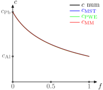
Figure 1: Effective speed $c$ versus concentration $f_{\mathrm{Al}}$ for conjugated Al/Pb and Pb/Al lattices of 0^∘-oriented rods. The numerical curves for both lattices (computed via (52) with $N=25$ and $m=10$), the PWE estimate (53), the MM estimate (49) and the MST approximations (54), (55) all merge at the scale of the plot.

In this subsection, a comparison between the numerical evaluation of the effective speed $c$ and its different estimates is demonstrated for several examples of a square lattice of parallel square rods embedded in a matrix and oriented at an angle of 0^∘ or 45^∘ to the translation vectors. Such configurations of phononic crystals have been studied, e.g., in GV ; WLL ; F-M ; F-MM ; M-B . It is clear that the MST estimate of MLWS ; TS ; SMLW ; TS1 , though derived for cylindrical inclusions, should be equally viable for square ones since it describes the quasistatic limit. If the contrast of matrix and inclusion shear coefficients is relatively low, then so is the difference between the two values of the effective speed $c$ for the two conjugated lattices. In this case, the PWE, MM and MST estimates (53), (49) and (54)-(55) all yield close values that provide a good approximation of $c$ in either of the conjugated configurations. This is exemplified in Fig. 1 for Al and Pb phases with the material constants $\rho_{\mathrm{Al}}=2.7$, $\rho_{\mathrm{Pb}}=11.6~{}$g/cm³ and$\ \mu_{\mathrm{Al}}=26$, $\mu_{\mathrm{Pb}}=14.9$ GPa. Note that the series (52) needs only about $j\sim 7$ modes ($N\sim 15$) and $m\sim 5$ terms for accurate calculation of the numerical curve $c\left(f_{\mathrm{Al}}\right)$ (the larger values of $N$ and $m$ indicated in the caption were taken for better precision).

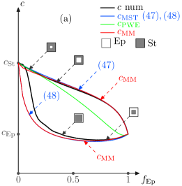
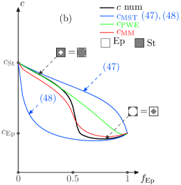
Figure 2: Effective speed (a) for the conjugated St/Ep and Ep/St lattices of 0^∘-oriented rods and (b) for the symmetric St/Ep lattice of 45^∘-rotated rods. Numerical curves $c\left(f_{\mathrm{Ep}}\right)$ are computed via (52) with $N=841$ and $m=150$; the PWE estimate $c_{\mathrm{PWE}}$ is given by (53); the MM estimate $c_{\mathrm{MM}}$ is given by (49); the MST approximations $c_{\mathrm{MST}}^{(\mathrm{St/Ep})}$ and $c_{\mathrm{MST}}^{(\mathrm{Ep/St})}$ are given by (54) and (55) with $J=1=\mathrm{St}$, $J=2=\mathrm{Ep.}$

Addressing the high-contrast case, consider two examples of binary materials with a ’medium’ and ’drastic’ contrast: one consisting of steel ($\equiv$ St) and epoxy ($\equiv$ Ep), and the other of steel and rubber ($\equiv$ R). Their material constants are $\rho_{\mathrm{St}}=7.8$, $\rho_{\mathrm{Ep}}=1.14$, $\rho_{\mathrm{R}}=1.14\$g/cm${}^{3}\$and $\mu_{\mathrm{St}}=80$, $\mu_{\mathrm{Ep}}=1.48$, $\mu_{\mathrm{R}}=4\cdot 10^{-5}\$GPa. The results for the St/Ep and Ep/St conjugated lattices of 0^∘-oriented rods are shown in Fig. 2a, and the results for the St/R and R/St lattices are shown in Fig. 3a. It is seen that the two numerical curves $c\left(f\right),$ plotted for each conjugated pair as a function of concentration of the same (say, softer) material, have quite different trajectories between the fixed end points. The physical reason is obvious: the effective speed $c$ is indeed strongly affected by a small concentration of a highly contrasting component when this forms a ’network’ breaking up connectivity of the volume-dominating component. On the numerical side, given the ’medium-contrast’ case of steel-epoxy composite, Eq. (52) provides a reasonable approximation of $c\left(f\right)$ when taken with $j=7$ modes ($N\sim 15$) and $m\sim 50$ terms (compare with the above Al-Pb case). About this number of modes and terms in Eq. (52) is also sufficient to capture the shape of the curve $c\left(f\right)$ for the ’drastic-contrast’ steel-rubber structure but only if rubber is an inclusion located inside the cell. Markedly more numerical effort is required when rubber is the matrix material distributed along the unit-cell boundaries - in this case no less than $j=12$ modes ($N\sim 25$) and $m\sim 150$ terms in Eq. (52) are needed to obtain good accuracy (see § 4). Note that formally reducing $\mu_{\mathrm{R}}$ to zero causes no discernible changes at the scale of Figs. 3, 4.

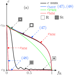
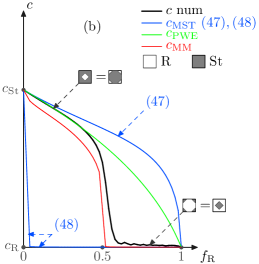
Figure 3: The same as in Fig. 2 (a,b) but for St/R and R/St lattices. Numerical curves $c\left(f_{\mathrm{R}}\right)$ are computed via (52) with $N=29$ and $m=150$. Note that $c_{\mathrm{R}}$ is not distinguishable from $0$ at the scale of the vertical axis.

Let us now examine the PWE, MM and MST estimates of $c$ for the above examples. It is evident that a single curve of the PWE estimate, which depends only on volume fraction and disregards geometrical details (see §V.1.1), cannot fit two markedly different curves of conjugated lattices. As noted in §III, it must be more accurate when the stiff component is volumetrically dominant over the soft one rather than when the situation is reversed. This is what is observed in Figs. 2a and 3a. It is also seen that the MM and MST estimates provide a fairly close evaluation of $c,$ which fits very well the whole numerical curve of $c$ for St/Ep and St/R lattices (soft rods in stiff matrix); however, they lose accuracy for the conjugated, Ep/St and R/St lattices (stiff rods in soft matrix), specifically when the rod concentration $f_{\mathrm{St}}$ ($=1-f_{\mathrm{Ep,R}}$) is close to 1. Regarding MST, this is in agreement with the remark made on its derivation in MLWS ; TS ; SMLW ; TS1 that the MST estimate does not fully account for the multiple interactions and hence may be error prone in the case of densely packed stiff inclusions. Thus, in the latter case, the PWE estimate is preferable to two others, as illustrated in Fig. 2a and especially in Fig. 3a.

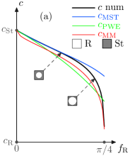
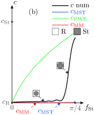
Figure 4: Effective speed as a function of concentration of inclusions in (a) St/R and (b) R/St conjugated lattices of circular cylinders in a matrix. Numerical curves $c\left(f_{\mathrm{R}}\right)$ and $c\left(f_{\mathrm{St}}\right)$ are computed via (52) with $N=29$ and $m=150$.

Consider next similar structures but with 45^∘-rotated rods, which is the case where the two conjugated lattices coincide into one symmetric configuration. The corresponding dependence of the effective speed versus concentration $c\left(f\right)$ has a single-valued approximation for each of the PWE and MM estimates, whereas the MST estimate still defines two different approximations (54) and (55) for the single curve $c\left(f\right)$. Comparing these estimates displayed alongside the numerical curve $c\left(f\right)$ in Figs. 2b and 3b shows that the PWE estimate is the most accurate so long as the stiff component is volume-dominant; the MM estimate provides the best ’overall’ fit; and each of the MST approximations works over less than a half of the range while mismatching markedly the other half.

Finally, we consider the case of cylindrical inclusions. Results for the steel - rubber conjugate lattices with circular rods are presented in Fig. 4. It is instructive to observe the similarity of the dependences $c\left(f\right)$ on the concentration of inclusions $f=f_{\mathrm{St}}$ and $f_{\mathrm{R}},$ which are displayed in Figs. 4a and 4b, to the two corresponding ’halves’ of the corresponding curves for square rods in Fig. 3b.

V.2 Three-phase lattices

V.2.1 Estimates

Consider a 2D square lattice similar to above but with a coated inclusion. Such nested structures have received much attention lately in relation to modelling locally resonant phononic crystals, e.g. LCS ; LPDV . The PWE and MM estimates of the effective speed $c$ for this case are given by Eqs. (24₂) and (49) with $\left\langle\cdot\right\rangle=\sum_{J}\left(\cdot\right)_{J}f_{J}$ and $J=1,2,3$. If the concentration $f_{J}$ of one of the constituent materials tends to zero, the MM estimate (49) for three constituents certainly tends to that for two remaining constituents; whereas the PWE estimate (24₂) with, say, $f_{3}\rightarrow 0$ tends to its form for the pair $J=1,2$ only if the ’vanishing’ material is neither the stiffest nor the softest one, i.e. if $\mu_{3}\neq\mu_{\min},$ $\mu_{\max}$.

As a MST counterpart, we adopt the generalization of (54) that is well-known in micromechanics as the Kuster-Toksöz formula (closely related to Hashin-Shtrikman bounds) for 2D fluids with small concentration of different inclusions KT ; B . More recently, it was used for a periodic structure of different cylinders in a fluid matrix TS ; TS1 . The formula for the 2D configurations considered here is

$$c^{2} \approx c_{\mathrm{MST}}^{2}=\frac{\mu_{1}}{\left\langle\rho\right\rangle}\left(\frac{1-\sum\nolimits_{J=2}^{3}f_{J}\frac{\mu_{1}-\mu_{J}}{\mu_{1}+\mu_{J}}}{1+\sum\nolimits_{J=2}^{3}f_{J}\frac{\mu_{1}-\mu_{J}}{\mu_{1}+\mu_{J}}}\right),$$ (57)

$$J = 1\mathrm{\ is\ matrix,\ }J=2,3\mathrm{\ are\ inclusions.}$$

The MST estimate (57) coincides with the binary formula (54) if any one of the inclusion concentrations $f_{2}$ or $f_{3}$ is zero. On the other hand, (57) does not tend to either of (54) and (55) as the matrix concentration $f_{1}$ tends to zero (which is not surprising since the Kuster-Toksöz is not recommended at low matrix concentration B2 ).

V.2.2 Examples

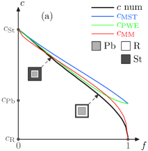
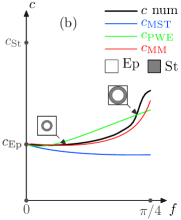
Figure 5: Effective speed $c\left(f\right)$ for three-phase lattices where $f$ is given by (58) with $\alpha=4/9$: (a) Pb/Ru/St structure of coated square rods and (b) Ep/St/Ep structure of cylindrical annuli. Numerical curves are computed via (52) with $N=29$ and $m=150$

Denote the filling fraction of a coated inclusion in a matrix ($J=1$) by $f$ and set the filling fractions of the skin ($J=2$) and core ($J=3$) materials as

$$f_{2}=\alpha f\ \ (\mathrm{skin}),\ f_{3}=\left(1-\alpha\right)f\ \ (\mathrm{core})\ \Rightarrow\ f_{2}+f_{3}=f.$$ (58)

The effective speed $c$ of the three-phase composite is now a function of the single variable $f=1-f_{1}$.

Motivated by LCS ; LPDV , we first examine the case of a soft coating (skin) material. Consider the square St/R/Pb lattice of square lead ($\equiv$Pb) rods coated by rubber ($\equiv$R) which are embedded in steel matrix (Fig. 5a). The value of $c\left(f\right)$ at $f=0$ is obviously the speed in the matrix, $c\left(0\right)=c_{\mathrm{St}}$. The opposite limit value of $c\left(f\right)$ at $f=1$ is equal to the effective speed $c_{\mathrm{R/Pb}}\left(f_{\mathrm{R}}\right)$ in the binary R/Pb lattice of lead rods embedded in the rubber matrix with the volume fractions fixed by (58) as $f_{\mathrm{R}}=\alpha$ and $f_{\mathrm{Pb}}=1-\alpha$. Once $f_{\mathrm{R}}$ is not too small, $c_{\mathrm{R/Pb}}\left(f_{\mathrm{R}}\right)$ should be close to $c_{\mathrm{R}}$ (see Fig. 3a), which therefore implies that $c\left(f\right)$ in the St/R/Pb structure has a very small value in the limit $f\rightarrow 1$. This is observed in Fig. 5a (where $\alpha=4/9$). It is also seen that the PWE and MST estimates (24₂) and (57) of $c(f)$ do not describe this behaviour of $c(f)$ at $f\rightarrow 1$ and overestimate $c\left(1\right)$ (by an incidentally close value which is neither PWE nor MST estimate of $c_{\mathrm{R/Pb}}\left(f_{\mathrm{R}}\right)$, as pointed out in §V.2.1 above). By contrast, the MM estimate (49) provides a good fit for the whole curve $c\left(f\right)$ including the critical region $f\rightarrow 1$. This is because Eq. (49) captures the ’insulating’ effect of a small concentration of soft material which drastically decreases the effective speed when this material extends throughout the unit-cell boundary, see §III.2.

Another case of interest is when the matrix material coincides with that of the rod core, which means that the rod coatings are simply spacers separating the same material. Figure 5b demonstrates the dependence of the effective speed $c$ on the concentration $f$ of stiff (steel) cylindrical annuli embedded in a soft (epoxy$\equiv$Ep) material. The shape of the curve $c\left(f\right)$ can be shown to change only slightly if the steel spacers are square instead of circular. It is seen from Fig. 5b that the basic outline of this curve is again best approximated by the MM estimate.

VI Conclusion

The paper uses the PWE approach and a newly developed MM approach, based on the monodromy matrix, to derive the new estimates of the effective shear-wave speed $c$ in 2D periodic lattices. The estimates are compared with the known MST approximations and with the numerical data for a number of examples of two- and three-phase square lattices. The main findings are listed in the Introduction. The results for effective velocities of the vector waves in the 3D lattices are to be reported elsewhere. It is worth pointing out that the obtained PWE and MM estimates are also valid for the gradient-index, or functionally graded, materials (for which the MST is irrelevant). In conclusion, the combination of the perturbation theory with the PWE and MM techniques, which is elaborated in this paper, is hoped to lend an efficient tool for a broad range of problems concerned with periodic composites, phononic crystals and metamaterials.

Acknowledgement. This work has been supported by the grant ANR-08-BLAN-0101-01 from the Agence Nationale de la Recherche and by the project SAMM from the cluster Advanced Materials in Aquitaine. A.N.N. acknowledges the support by the Centre National de la Recherche Scientifiqueis.

APPENDIX. Convergence of (20₂): a strict example

Sufficient condition on $\mu(\mathbf{x})$. Our objective is to provide a rigorous example of a class of functions $\mu\left(\mathbf{x}\right)\equiv\mu_{0}+\mu_{\Delta}\left(\mathbf{x}\right)$ that guarantee convergence for $M(\mathbf{\kappa})=\mu_{0}^{-1}\sum\nolimits_{n=0}^{\infty}\left(\left(-\mathbf{C}\right)^{n}\mathbf{f,f}\right)$, and thus validate application of this series for computing the effective parameters $\mu_{\mathrm{eff}}(\mathbf{\kappa})$ and $c^{2}(\mathbf{\kappa})$. To do so, we begin by formulating a sufficient condition on $\mu\left(\mathbf{x}\right)$ to fulfill the sufficient condition $\left\|\mathbf{C}(\mu_{0})\right\|<1$ for convergence of (20₂) as $m\rightarrow\infty$. Note that the matrix $\mathbf{\mathbf{C}}$ can be written as

$$\mathbf{C}=\mu_{0}^{-1}\sum\nolimits_{\widetilde{\mathbf{g}}\in\Gamma}\widehat{\mu}_{\Delta}\left(\widetilde{\mathbf{g}}\right)\mathbf{J}_{\widetilde{\mathbf{g}}}\ \ \mathrm{where\ }\mathbf{J}_{\widetilde{\mathbf{g}}}\mathrm{:}$$

$$J_{\widetilde{\mathbf{g}}}\left[\mathbf{\mathbf{g,g}}^{\prime}\right]=\begin{cases}\frac{\mathbf{g}}{\left|\mathbf{g}\right|}\cdot\frac{\mathbf{g}^{\prime}}{\left|\mathbf{g}^{\prime}\right|}&\mathrm{if}\mathbf{\mathbf{\ \widetilde{\mathbf{g}}=\mathbf{g-g}^{\prime},}}\\ 0\ &\mathrm{otherwise}\mathbf{.}\end{cases}$$ (59)

It is seen from (59) that $\left\|\mathbf{\mathbf{C}}\right\|\leq\mu_{0}^{-1}\sum\nolimits_{\widetilde{\mathbf{g}}\in\Gamma}\left|\widehat{\mu}_{\Delta}\left(\widetilde{\mathbf{g}}\right)\right|$ since $\left\|\mathbf{J}_{\widetilde{\mathbf{g}}}\right\|\leq 1,$ which in turn is because all its nonzero elements $J_{\widetilde{\mathbf{g}}}\left[\mathbf{\mathbf{g,g}}^{\prime}\right]$ occupy a single particular diagonal and satisfy $\left|J_{\widetilde{\mathbf{g}}}\left[\mathbf{\mathbf{g,g}}^{\prime}\right]\right|\leq 1$. Hence the sufficient convergence condition $\left\|\mathbf{C}\right\|<1$ may be eased to

$$\left(\left\|\mathbf{C}(\mu_{0})\right\|\leq\right)~{}\mu_{0}^{-1}\sum\nolimits_{\widetilde{\mathbf{g}}\in\Gamma}\left|\widehat{\mu}_{\Delta}\left(\widetilde{\mathbf{g}}\right)\right|=1-\frac{\left\langle\mu\right\rangle}{\mu_{0}}\\ +\frac{1}{\mu_{0}}\sum\nolimits_{\mathbf{g}\neq\mathbf{0}}\left|\widehat{\mu}\left(\mathbf{g}\right)\right|\equiv\Theta_{\mu_{0}}<1\ \mathrm{for}\ \ \mu_{0}\geq\left\langle\mu\right\rangle.$$ (60)

In other words, for those $\mu(\mathbf{x})$ which satisfy

$$\sum\nolimits_{\mathbf{g}\neq\mathbf{0}}\left|\widehat{\mu}\left(\mathbf{g}\right)\right|<\left\langle\mu\right\rangle$$ (61)

there always exists a choice of $\mu_{0}\geq\left\langle\mu\right\rangle$ which ensures $\left\|\mathbf{C}(\mu_{0})\right\|<1$ and hence guarantees convergence of (20₂) to $M\left(\mathbf{\kappa}\right)$. The remainder of the series (20₂) with $\mu_{0}\geq\left\langle\mu\right\rangle$ may be estimated as follows

$$\left|\mu_{0}^{-1}\sum\nolimits_{n=m+1}^{\infty}\left(\left(-\mathbf{C}\right)^{n}\mathbf{f,f}\right)\right|\leq\frac{\left\|\mathbf{f}\right\|^{2}}{\mu_{0}}\sum\nolimits_{n=m+1}^{\infty}\left\|\mathbf{C}\right\|^{n}$$

$$<\frac{\left\langle\mu\right\rangle^{2}}{\mu_{0}}\frac{\Theta_{\mu_{0}}^{m+1}}{1-\Theta_{\mu_{0}}}=\frac{\left\langle\mu\right\rangle^{2}\Theta_{\mu_{0}}^{m+1}}{\left\langle\mu\right\rangle-\sum\nolimits_{\mathbf{g}\neq\mathbf{0}}\left|\widehat{\mu}\left(\mathbf{g}\right)\right|},$$ (62)

where it has been used that $\left\|\mathbf{C}\right\|\leq$ $\Theta_{\mu_{0}}$ by (60) and that

$$\left\|\mathbf{f}\right\| = \sqrt{\left\langle\left|f\left(\mathbf{x}\right)\right|^{2}\right\rangle}\leq\max\limits_{\mathbf{x}}\left|f\left(\mathbf{x}\right)\right|$$

$$\leq \sum\nolimits_{\mathbf{g}\neq\mathbf{0}}\left|\widehat{\mu}\left(\mathbf{g}\right)e^{i\mathbf{g\cdot x}}\frac{\mathbf{g}}{\left|\mathbf{g}\right|}\cdot\mathbf{\kappa}\right|<\left\langle\mu\right\rangle$$

for$\ f\left(\mathbf{x}\right)=\sum\nolimits_{\mathbf{g}\neq\mathbf{0}}\widehat{f}\left(\mathbf{g}\right)e^{i\mathbf{g\cdot x}}$ by (14) and (61). The least value of the residual sum (62) for all $\mu_{0}\geq\left\langle\mu\right\rangle$ is achieved when $\Theta_{\mu_{0}}$ is minimum, which is the case when $\mu_{0}=\left\langle\mu\right\rangle$. Note that the average $\left\langle\mu\right\rangle$ of $\mu(\mathbf{x})$ satisfying (61) may well differ (be greater or less) than the value $\overline{\mu}\equiv\frac{1}{2}\left(\mu_{\max}+\mu_{\min}\right),$ which was argued in §IV as a numerically reliable choice of $\mu_{0}$ in (20₂). There is indeed no contradiction in this difference. First, recall that all the conclusions of Appendix stem from only the sufficient conditions. Second, as mentioned in §IV, an advantage of taking (20₂) with $\mu_{0}=\overline{\mu}$ is that it yields the same formula (52) for any profile $\mu(\mathbf{x})$, but this choice of $\mu_{0}$ is not intended to provide the fastest convergence for all possible profiles.

We still need to examine the restrictions on $\mu\left(\mathbf{x}\right)$ which are imposed by the derived sufficient condition (61). First of all, by (61) $\mu(\mathbf{x})=\sum\nolimits_{\mathbf{g}}\widehat{\mu}\left(\mathbf{g}\right)e^{i\mathbf{g\cdot x}}\geq$ $\widehat{\mu}\left(\mathbf{0}\right)-\sum\nolimits_{\mathbf{g}\neq\mathbf{0}}\left|\widehat{\mu}\left(\mathbf{g}\right)\right|>0,$ i.e. only positive $\mu(\mathbf{x})$ are allowed as needed. Second, any $\mu(\mathbf{x})$ satisfying (61) must have a uniformly converging Fourier series and hence be continuous. The latter is actually not a loss of generality in the numerical context, even if we are mostly interested in the case of materials with inclusions (i.e. with jumps of properties), because the calculations deal with truncated Fourier series of $\mu(\mathbf{x})$ which in effect replaces a possibly piecewise constant $\mu(\mathbf{x})$ by a continuous profile. Thirdly, (61) implies that $\left|\mu(\mathbf{x})-\left\langle\mu\right\rangle\right|\leq\left\langle\mu\right\rangle$, i.e. $\mu(\mathbf{x})>0$ should not depart ’too far’ from its average $\left\langle\mu\right\rangle.$ When so, the matrix $\mathbf{I+C}$ is diagonal predominant and $\left|\mathbf{f}\right|$ decreases for large $\mathbf{g,}$ both furthering the truncation of the PWE and of the power series in (20₂). It is evident that the above condition, which may be recast as $\mu_{\max}\leq 2\left\langle\mu\right\rangle,$ fits a fairly broad class of functions $\mu(\mathbf{x})$.

Example. In constructing an explicit example of the profile $\mu(\mathbf{x})$ which ensures convergence of (20₂), we consider one that emulates a high-contrast composite with a small volume fraction of soft inclusions. For brevity of writing, let $\mathbf{T}=\left[-\pi,\pi\right]^{2}$ so that $\mathbf{x}=\left(x_{1},x_{2}\right),$ $\mathbf{g}=\left(g_{1},g_{2}\right)$ with $x_{i}\in\left[-\pi,\pi\right]$ and $g_{i}=n_{i}$ ($n_{i}\in\mathbb{Z}$). Denote

$$\varphi_{n_{1}n_{2}}\left(\mathbf{x}\right)=\psi_{n_{1}}\left(x_{1}\right)\psi_{n_{2}}\left(x_{2}\right)=\\ \sum\nolimits_{\left|g_{1}\right|\leq n_{1};~{}\left|g_{2}\right|\leq n_{2}}\widehat{\varphi}_{n_{1}n_{2}}\left(\mathbf{g}\right)e^{i\mathbf{g\cdot x}},\\ \mathrm{where}\ \psi_{n}\left(x\right)\equiv\left(\cos x\right)^{2n}=\sum\nolimits_{\left|g\right|\leq n}\widehat{\psi}_{n}\left(g\right)e^{igx}.$$ (64)

Since $\psi_{n}\left(\pi l\right)=1$ ($l\in\mathbb{Z}$) and $\psi_{n}\left(x\right)\rightarrow 0$ for $x\neq\pi l$ as $n\rightarrow\infty$, the function $\varphi_{n_{1}n_{2}}\left(x_{1},x_{2}\right)$ for large $n_{1}$, $n_{2}$ tends to a 2D grid of narrow unit peaks. Note also that $\widehat{\psi}_{n}\left(g\right)\geq 0\ \forall g$ and $\sum\nolimits_{\left|g\right|\leq n}\widehat{\psi}_{n}\left(g\right)=\psi_{n}\left(0\right)=1$, whence $\widehat{\varphi}_{n_{1}n_{2}}\left(\mathbf{g}\right)\geq 0$ and $\sum\nolimits_{\left|g_{1}\right|\leq n_{1},~{}\left|g_{2}\right|\leq n_{2}}\widehat{\varphi}_{n_{1}n_{2}}\left(\mathbf{g}\right)=1$. Using this $\varphi_{n_{1}n_{2}}$, define the function $\mu(\mathbf{x})$ as follows:

$$\mu(\mathbf{x})=\mu_{0}+\mu_{\Delta}\left(\mathbf{x}\right):\\ \mu_{0}>A>0,\ \mu_{\Delta}\left(\mathbf{x}\right)=-A\varphi_{n_{1}n_{2}}\left(\mathbf{x}\right),$$ (65)

where $\mu_{0}$ and $A$ are some constants. From the above properties it follows that

$$\sum\nolimits_{\mathbf{g\neq 0}}\left|\widehat{\mu}\left(\mathbf{g}\right)\right|=A\sum\nolimits_{\mathbf{g\neq 0}}\widehat{\varphi}_{n_{1}n_{2}}\left(\mathbf{g}\right)=\\ A\left(1-\widehat{\varphi}_{n_{1}n_{2}}\left(\mathbf{0}\right)\right)<\mu_{0}-A\widehat{\varphi}_{n_{1}n_{2}}\left(\mathbf{0}\right)=\left\langle\mu\right\rangle.$$ (66)

Thus the function (65) satisfies the condition (61) sufficient for convergence of (20₂).

References

• (1) Y. Benveniste and G.W. Milton, J. Mech. Phys. Solids 58, 1026 (2010).
• (2) P. A. Martin, A. Maurel and W. J. Parnell, J.Β Acoust. Soc. Am. 128, 571 (2010).
• (3) W. J. Parnell and I. D. Abrahams, Waves Random Complex Media 20, 678 (2010).
• (4) A. A. Krokhin, J. Arriaga and L. N. Gumen, Phys. Rev. Lett. 91, 264302 (2003).
• (5) I. V. Andrianov, V. I. Bolshakov, V. V. Danishevsβ€˜kyy and D.Weichert, Proc. Roy. Soc. A 464, 1181 (2008).
• (6) S. Nemat-Nasser, J. R. Willis, A. Srivastava and A. V. Amirkhizi, Phys. Rev. B 83, 104103 (2011).
• (7) J. Mei, Z. Liu, W. Wen and P. Sheng, Phys. Rev. Lett. 96, 024301 (2006); Phys. Rev. B 76, 134205 (2007).
• (8) D. Torrent and J. SΓ‘nchez-Dehesa, Phys. Rev. B 74, 224305 (2006).
• (9) P. Sheng, J. Mei, Z. Liu and W. Wen, Physica B 394, 256 (2007).
• (10) D. Torrent and J. SΓ‘nchez-Dehesa, New J. Phys. 9, 323 (2007); ibid. 10, 023004 (2008).
• (11) N. S. Bakhvalov and G. Panasenko, Homogenisation: Averaging Processes in Periodic Media - Mathematical Problems in the Mechanics of Composite Materials (Kluwer Academic Publishers, 1989).
• (12) M. C. Pease, III, Methods of Matrix Algebra (Academic Press, New York, 1965).
• (13) A. A. Kutsenko, A. L. Shuvalov, A. N. Norris and O. Poncelet, submitted.
• (14) J. O.Β Vasseur, P. A. Deymier, B. Djafari-Rouhani, Y. Pennec and A.-C. Hladky-Hennion, Phys. Rev. B 77, 085415 (2008).
• (15) Z. Hashin, J. Appl. Mech. 50, 481-505 (1983).
• (16) J.E. Flaherty and J.B. Keller, Comm. Pure Appl. Math. 26, 565 (1973).
• (17) G. W. Milton, The Theory of Composites (Cambridge University Press, 2001).
• (18) C. Goffaux and J. P. Vigneron, Phys. Rev. B 64, 075118 (2001).
• (19) F. G. Wu, Z. Y. Liu and Y. Y. Liu, Phys. Rev. E 66, 046628 (2002).
• (20) L. Feng, X.-P. Liu, M.-H. Lu, Y.-B. Chen, Y.-F. Chen, Y.-W. Mao, J. Zi, Y.-Y. Zhu, S.-N. Zhu and N.-B. Ming, Phys. Rev. B 73, 193101 (2006).
• (21) M. Farhat, S. Guenneau, S. Enoch, G. Tayeb, A. B. Movchan and N. V. Movchan, Phys. Rev. E 77, 046308 (2008).
• (22) B. Manzanares-Martinez, F. Ramos-Mendieta and A. Baltazar, J. Acoust. Soc. Am. 127, 3503 (2010).
• (23) N. Swinteck, J.-F. Robillard, S. Bringuier, J. Bucay, K. Muralidharan, J. O. Vasseur, K. Runge and P. A. Deymier, Appl. Phys. Lett. 98, 103508 (2011).
• (24) Z. Liu, C. T. Chan and P. Sheng, Phys. Rev. B 71, 014103 (2005).
• (25) H. Larabi, Y. Pennec, B. Djafari-Rouhani and J. O.Β Vasseur, Phys. Rev. E 75, 066601 (2007).
• (26) T. Kuster and M. N. ToksΓΆz, Geophysics 39, 587 (1974).
• (27) J.G. Berryman, J. Acoust. Soc. Am. 68, 1809 (1980).
• (28) J.G. Berryman, Mech. Materials 22, 149 (1996).