Non-equilibrium entangled steady state of two independent two-level systems

Abstract

We determine and study the steady state of two independent two-level systems weakly coupled to a stationary non-equilibrium environment. Whereas this bipartite state is necessarily uncorrelated if the splitting energies of the two-level systems are different from each other, it can be entangled if they are equal. For identical two-level systems interacting with two bosonic heat baths at different temperatures, we discuss the influence of the baths temperatures and coupling parameters on their entanglement. Geometric properties, such as the baths dimensionalities and the distance between the two-level systems, are relevant. A regime is found where the steady state is a statistical mixture of the product ground state and of the entangled singlet state with respective weights 2/3 and 1/3.

I Introduction

For a quantum system, the influence of the surroundings plays a role at a fundamental level. When the environment is taken into consideration, the system dynamics can no longer be described in terms of pure quantum states and unitary evolution. An open quantum system is generally in a statistical mixture of pure states. This has an important consequence for multipartite systems. As is well known, correlations between quantum systems cannot be completely understood in classical terms W . There exist states which are not classically correlated and lead to correlations with no classical counterpart, as clearly shown by violations of Bell inequalities for instance B . They are said to be entangled. Whereas almost all pure states are entangled, this is not the case for mixed states. In the space of mixed states, the set of non-entangled, or separable, states has a finite volume ZHSL . An interesting consequence of the geometrical properties of this set is that the state of a multipartite open system can be entangled for finite periods of time, in the course of its evolution, and separable at infinite time or vice versa TC .

The most common environment is a heat reservoir. If the considered system is weakly coupled to an infinite number of degrees of freedom, initially in thermal equilibrium, it relaxes, in general, to a thermal state with the temperature of its surroundings. In such an environment, it is clear that, in the absence of direct interactions between the subsystems of a multipartite system, these subsystems are uncorrelated at long times. In other words, any initial correlation, quantum or classical, between independent subsystems is generically destroyed by a thermal bath. Moreover, for the geometric reasons mentioned above, quantum disentanglement can occur in a finite time YE ; JJ . Furthermore, the disentangling influence of the environment also exists when no energy is exchanged between the system and its surroundings, whereas, in this particular case, classical correlations can persist DH ; YEPRB .

However, when independent systems interact with a common environment, the indirect interaction between them, mediated by this environment, may have a positive impact on their entanglement. Recent results evidence the existence of this influence. It has been shown that a transient entanglement, between initially uncorrelated systems, can be induced by a thermal bath, for both non-dissipative Br and dissipative J ; BFP ; MCNBF couplings. It has also been obtained that, in the limit of infinitely close non-interacting systems, some special entangled states are not affected by the environment ZR . In this limiting case, the considered multipartite open system has not a unique steady state, which is exceptional, and hence the entanglement evolution depends on the system’s initial state.

In the above cited dynamical studies, the environment is in thermal equilibrium and thus a relaxation dynamics towards a unique steady state necessarily means decay of correlations, both quantum and classical, between non-interacting systems. This may not be the case for a non-equilibrium surroundings. Stationary entanglement has been found in the presence of particle HDB ; CPA or energy flow PH ; KAM . However, in these studies, entanglement occurs between systems that interact with each other directly, via a two-level system, or via strong coupling to a heat bath, and this interaction plays an essential part in the development of entanglement. Such a strong interaction has been shown to be unnecessary for a different kind of non-equilibrium environment CKS . In the presence of a classical oscillating field, the steady state of two two-level atoms, interacting with each other only via weak coupling to the electromagnetic vacuum, can be entangled.

In this paper, we consider two independent two-level systems (TLS) coupled to a steady non-equilibrium environment. Examples of such surroundings are illustrated in Fig.1. They consist of several heat baths at different temperatures. These are not the only possible examples and the two following sections are relevant to other environments. In section II, we present the model used to describe two non-interacting TLS in a stationary environment. In section III, we first study the steady state of a general system weakly coupled to its surroundings, and we then apply our approach to the case of a system consisting of two independent TLS. The system steady state is obtained, in the weak coupling limit, by solving perturbatively an eigenvalue problem, which is derived from the system dynamics for arbitrary coupling strength. As far as one is interested only in the stationary state, no other approximation, such as a Markovian assumption, or elaborate method, such as a projection superoperator technique, are needed QDS ; CDG . In section IV, we focus on the special case of an environment that consists of bosonic heat baths at different temperatures. It is shown that two baths are enough to induce stationnary entanglement of two identical TLS. The influence of the two baths temperatures and of the coupling parameters is discussed in some detail. Finally, we summarize our results in the last section.

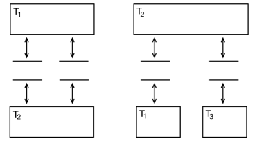
Figure 1: Schematic representation of non-equilibrium environments of two independent TLS. The depicted environments consist of several heat baths at different temperatures.

II Model

The total Hamiltonian of two independent TLS and their environment ${\cal E}$ can be written as

$$H=\sum_{i=1}^{2}\left[-\frac{\Delta_{i}}{2}\sigma_{z}^{(i)}+v_{i}\sigma_{z}^{(i)}+w_{i}\sigma_{+}^{(i)}+w^{{\dagger}}_{i}\sigma_{-}^{(i)}\right]+H_{\cal E}$$ (1)

where $\Delta_{i}$ are the level splittings of the TLS, $v_{i}=v_{i}^{{\dagger}}$ and $w_{i}$ are operators of ${\cal E}$ and $H_{\cal E}$ is the self-Hamiltonian of ${\cal E}$. The Pauli operator $\sigma_{z}^{(i)}$ has eigenvalues $\pm 1$ and the corresponding eigenstates are denoted by $|\pm\rangle_{i}$. The operators $\sigma_{\pm}^{(i)}$ then read $\sigma_{+}^{(i)}=[\sigma_{-}^{(i)}]^{{\dagger}}=|+\rangle_{i}{{}_{i}}\langle-|$. We introduce, for further use, the following notations :

$$|1\rangle=|+\rangle_{1}|+\rangle_{2} |2\rangle=|+\rangle_{1}|-\rangle_{2},$$ ,

$$|3\rangle=|-\rangle_{1}|+\rangle_{2} |4\rangle=|-\rangle_{1}|-\rangle_{2}.$$ , (2)

Two TLS interacting with their environment but not directly with each other can always be described by a Hamiltonian of the form (1). The system ${\cal E}$ is assumed to consist of an infinite number of degrees of freedom and to lead to a decohering and dissipative reduced dynamics of the TLS.

As the initial state of the complete system, we consider

$$\Omega=\sum_{k,l}r_{kl}|k\rangle\langle l|\otimes\rho_{\cal E}$$ (3)

where $\rho_{\cal E}$ commutes with $H_{\cal E}$. The two-TLS system and ${\cal E}$ are initially uncorrelated. As we will see below, the condition $[\rho_{\cal E},H_{\cal E}]=0$ implies the stationarity of relevant correlation functions of ${\cal E}$. Typical environments we are interested in are made up of several heat baths at different temperatures $T_{n}$, as sketched in Fig.1. In this case, the environment Hamiltonian and initial state read, respectively, as $H_{\cal E}=\sum_{n}H_{{\cal E}n}$ where $n$ runs over the heat reservoirs and $[H_{{\cal E}n},H_{{\cal E}n^{\prime}}]=0$, and $\rho_{\cal E}\propto\prod_{n}\exp(-H_{{\cal E}n}/T_{n})$, and commute with each other. Throughout this paper, we use units in which $\hbar=k_{B}=1$.

III Non-equilibrium steady state

In this section, we first derive a matrix equation for the steady state of a generic open system ${\cal S}$ initially uncorrelated with its environment ${\cal E}$. More explicit equations are then obtained for a steady environment and in the limit of weak coupling between ${\cal S}$ and ${\cal E}$. This weak coupling approach is applied to the two TLS described by the Hamiltonian (1). In this case, the steady state equation can be solved. The result is radically different for $\Delta_{1}\neq\Delta_{2}$ and $\Delta_{1}=\Delta_{2}$.

III.1 General case

In general, under the influence of its environment ${\cal E}$, a system ${\cal S}$ relaxes to a steady state determined by its self-Hamiltonian and by its interaction with ${\cal E}$. If ${\cal E}$ is in thermal equilibrium and ${\cal S}$ interacts with it weakly, this state does not depend on any detail of the intrinsic dynamics of ${\cal E}$ or of the coupling between ${\cal S}$ and ${\cal E}$. But, as we will see, this is a very particular case. To determine the steady state of ${\cal S}$, we first write its reduced density matrix, at positive times $t$, as

$$\rho(t)=\frac{i}{2\pi}\int_{\R+i\eta}dze^{-izt}\mathrm{Tr}_{\cal E}\left[\left(z-{\cal L}\right)^{-1}\Omega\right]$$ (4)

where $\mathrm{Tr}_{\cal E}$ denotes the partial trace over ${\cal E}$, $\eta$ is a positive real number, and $\Omega$ is the initial state of the total system ${\cal S}+{\cal E}$. The Liouvillian ${\cal L}$ is defined by ${\cal L}\ldots=[H,\ldots]$ where $H$ is the Hamiltonian of ${\cal S}+{\cal E}$. This Hamiltonian can be decomposed as $H=H_{\cal S}+H_{int}+H_{\cal E}$ where $H_{\cal S}$ and $H_{\cal E}$ are the self-Hamiltonians of ${\cal S}$ and ${\cal E}$, respectively, and $H_{int}$ accounts for the interaction between ${\cal S}$ and ${\cal E}$. The condition $\mathrm{Tr}_{\cal E}(\rho_{\cal E}H_{int})=0$ can be assumed without loss of generality. It can always be satisfied by appropriately redefining $H_{\cal S}$ and $H_{int}$. The eigenstates and eigenenergies of $H_{\cal S}$ will be denoted by $|k\rangle$ and $\epsilon_{k}$ in the following.

III.1.1 Steady state equation

For an initial state $\Omega$ of the form (3), the matrix elements ${\tilde{r}}_{kl}(z)=\langle k|\mathrm{Tr}_{\cal E}[(z-{\cal L})^{-1}\Omega]|l\rangle$ of the Laplace transform of $\rho$, are given by

$${\tilde{r}}_{kl}(z)=\sum_{k^{\prime},l^{\prime}}\Gamma_{kl,k^{\prime}l^{\prime}}(z)r_{k^{\prime}l^{\prime}}$$ (5)

where the functions

$$\Gamma_{kl,k^{\prime}l^{\prime}}(z)=\langle k|\mathrm{Tr}_{\cal E}\left[\left(z-{\cal L}\right)^{-1}|k^{\prime}\rangle\langle l^{\prime}|\otimes\rho_{\cal E}\right]|l\rangle$$ (6)

depend only on the environment part of the initial state (3). Equation (5) can be read as a matrix relation between two column vectors ${\bf r}$ and ${\tilde{\bf r}}(z)$ with elements $r_{kl}$ and ${\tilde{r}}_{kl}(z)$, respectively, and a square matrix ${\bf\Gamma}(z)$ whose elements are given by (6). An important feature of this matrix is that the column vector ${\bf v}$ with elements $v_{kl}=\delta_{kl}$ is always left eigenvector of ${\bf\Gamma}(z)$ with eigenvalue $z^{-1}$, i.e., $\sum_{k}\Gamma_{kk,k^{\prime}l^{\prime}}(z)=\delta_{k^{\prime}l^{\prime}}/z$ EPJB . This equality ensures the conservation of the trace of the density matrix $\rho$, and follows simply from $\sum_{k}\langle k|\mathrm{Tr}_{\cal E}(\ldots)|k\rangle=\mathrm{Tr}(\ldots)$. The matrix ${\bf\Gamma}(z)$ can thus be written as ${\bf\Gamma}(z)=z^{-1}{\bf u}(z){\bf v}^{T}+{\bf\Gamma}^{\prime}(z)$ where ${\bf v}^{T}{\bf\Gamma}^{\prime}(z)=0$ and ${\bf v}^{T}{\bf u}(z)=1$. The column vector ${\bf u}(z)$ is right eigenvector of ${\bf\Gamma}(z)$ with eigenvalue $z^{-1}$. Provided it has no pole on the real axis, the corresponding term of ${\bf\Gamma}(z)$ can be analytically continued in the lower half plane and gives a constant contribution to the time-evolved density matrix (4). Since ${\bf v}^{T}{\bf r}=\sum_{k}r_{kk}=1$ for any density matrix $\rho(0)$, this contribution does not depend on the initial state of ${\cal S}$. In summary, the steady state of the open system ${\cal S}$ is $\sum_{k,l}u_{kl}|k\rangle\langle l|$ where $u_{kl}$ are the elements of the column vector ${\bf u}$ determined by

$$\lim_{\eta\rightarrow 0^{+}}\left\{i\eta{\bf\Gamma}(i\eta)\right\}{\bf u}={\bf u}.$$ (7)

Note that the condition $[\rho_{\cal E},H_{\cal E}]=0$ was not used to derive this equation.

III.1.2 Weak coupling limit

To determine the steady state of ${\cal S}$ in the limit of weak coupling to ${\cal E}$, we first expand the matrix elements (6) in powers of the Liouvillian ${\cal L}_{int}\ldots=[H_{int},\ldots]$. We obtain

$$\Gamma_{kl,k^{\prime}l^{\prime}}(z)=\frac{1}{z-\epsilon_{k}+\epsilon_{l}}\left\{\delta_{k^{\prime}k}\delta_{l^{\prime}l}+i\frac{\gamma_{kl,k^{\prime}l^{\prime}}(z)}{z-\epsilon_{k^{\prime}}+\epsilon_{l^{\prime}}}\right\}$$ (8)

up to second order, where $\gamma_{kl,k^{\prime}l^{\prime}}(z)$ can be expressed in terms of the correlation functions $C^{kl}_{k^{\prime}l^{\prime}}(t)=\mathrm{Tr}[\rho_{\cal E}\exp(itH_{\cal E})h_{kl}\exp(-itH_{\cal E})h_{k^{\prime}l^{\prime}}]$ of the environment operators $h_{kl}=\langle k|H_{int}|l\rangle=h_{lk}^{\dagger}$, as

$$\gamma_{kl,k^{\prime}l^{\prime}}(z)=\int_{0}^{\infty}dte^{izt}\Big{\{}e^{it\omega_{l^{\prime}k}}C^{l^{\prime}l}_{kk^{\prime}}(t)+e^{it\omega_{lk^{\prime}}}C^{l^{\prime}l}_{kk^{\prime}}(-t)\Big{.}\\ \Big{.}-\sum_{j}\big{[}\delta_{ll^{\prime}}e^{it\omega_{lj}}C^{kj}_{jk^{\prime}}(t)+\delta_{kk^{\prime}}e^{it\omega_{jk}}C^{l^{\prime}j}_{jl}(-t)\big{]}\Big{\}}.$$ (9)

In this expression, we have used the notation $\omega_{kl}=\epsilon_{k}-\epsilon_{l}$. The stationarity of the correlation functions $C^{kl}_{k^{\prime}l^{\prime}}$ stems directly from the steady environment assumption $[\rho_{\cal E},H_{\cal E}]=0$. For the Hamiltonian (1) and with the definitions (2), $h_{11}=-h_{44}=v_{1}+v_{2}$, $h_{22}=-h_{33}=v_{1}-v_{2}$, $h_{13}=h_{24}=w_{1}$, $h_{12}=h_{34}=w_{2}$ and $h_{14}=h_{23}=0$.

In the absence of interaction between ${\cal S}$ and ${\cal E}$, the eigenvalue problem (7) reduces to $(\epsilon_{k}-\epsilon_{l})u_{kl}=0$. Consequently, the only matrix elements $u_{kl}$ with nonvanishing zeroth-order approximations are that for which $\epsilon_{k}=\epsilon_{l}$. Thus, if the energy spectrum $\{\epsilon_{k}\}$ is nondegenerate, the corresponding steady density matrix is diagonal in the basis $\{|k\rangle\}$. In the opposite case, there can exist coherences between states $|k\rangle$ of equal energy. The matrix elements $u_{kl}$ to zeroth order, are determined by the equations

$$\sum_{\epsilon_{k^{\prime}}=\epsilon_{l^{\prime}}}\gamma_{kl,k^{\prime}l^{\prime}}(i0^{+})u_{k^{\prime}l^{\prime}}=0$$ (10)

where $k$ and $l$ satisfy $\epsilon_{k}=\epsilon_{l}$. The remaining coherences $u_{kl}$ are at least of first order in $H_{int}$. By writing explicitly the coefficients $\gamma_{kl,k^{\prime}k^{\prime}}(i0^{+})$, it can be shown that, for an environment in thermal equilibrium, i.e., $\rho_{\cal E}\propto\exp(-H_{\cal E}/T)$, the thermal state $u_{kl}\propto\delta_{kl}\exp(-\epsilon_{k}/T)$ is solution of (10), even in the presence of degeneracy in the spectrum of $H_{\cal S}$, see Appendix.

III.2 Different splitting energies

For unequal nonzero $\Delta_{1}$ and $\Delta_{2}$, the spectrum of the Hamiltonian $H_{\cal S}=-\sum_{i}\Delta_{i}\sigma_{z}^{(i)}/2$ is non degenerate. The zeroth-order steady state of the TLS is thus a statistical mixture of the states (2). The relation (10) becomes

$$\left(\begin{array}[]{cccc}0&-{\tilde{\gamma}}_{1}^{-}&-{\tilde{\gamma}}_{2}^{-}&{\tilde{\gamma}}_{1}^{+}+{\tilde{\gamma}}_{2}^{+}\\ -{\tilde{\gamma}}_{1}^{-}&0&{\tilde{\gamma}}_{1}^{+}+{\tilde{\gamma}}_{2}^{-}&-{\tilde{\gamma}}_{2}^{+}\\ -{\tilde{\gamma}}_{2}^{-}&{\tilde{\gamma}}_{1}^{-}+{\tilde{\gamma}}_{2}^{+}&0&-{\tilde{\gamma}}_{1}^{+}\\ {\tilde{\gamma}}_{1}^{-}+{\tilde{\gamma}}_{2}^{-}&-{\tilde{\gamma}}_{2}^{+}&-{\tilde{\gamma}}_{1}^{+}&0\end{array}\right)\left(\begin{array}[]{c}p_{1}\\ p_{2}\\ p_{3}\\ p_{4}\end{array}\right)=0$$ (11)

where $p_{k}=u_{kk}$. The elements of the above matrix can be written as

$${\tilde{\gamma}}_{i}^{+/-}=2\pi\sum_{A,B}P_{A/B}|\langle B|w_{i}|A\rangle|^{2}\delta(E_{A}-E_{B}+\Delta_{i})$$ (12)

where $E_{A}$ and $|A\rangle$ denote the eigenenergies and eigenstates of $H_{\cal E}$, and $P_{A}$ are the eigenvalues of $\rho_{\cal E}$. The coefficients ${\tilde{\gamma}}_{i}^{+}$ and ${\tilde{\gamma}}_{i}^{-}$ are the Fermi golden rule rates of the TLS $i$ CDG .

The solution of (11) leads to a product steady state $\rho=\rho_{1}\otimes\rho_{2}$ where

$$\rho_{i}=({\tilde{\gamma}}_{i}^{+}+{\tilde{\gamma}}_{i}^{-})^{-1}\big{[}{\tilde{\gamma}}_{i}^{+}|+\rangle_{i}{{}_{i}}\langle+|+{\tilde{\gamma}}_{i}^{-}|-\rangle_{i}{{}_{i}}\langle-|\big{]}.$$ (13)

The two TLS are uncorrelated, to lowest order in $H_{int}$, when their splitting energies are different from each other. Moreover, the steady state $\rho_{i}$ of TLS $i$ is the same in the presence or absence of the other TLS. In the special case $\Delta_{2}=0$, the zeroth-order coherences $u_{12}$ and $u_{34}$ are a priori different from zero since $\epsilon_{1}=\epsilon_{2}$ and $\epsilon_{3}=\epsilon_{4}$. But, for an environment ${\cal E}$ consisting of several heat baths, it is shown in the Appendix that $\rho=\rho_{1}\otimes I/4$ where $\rho_{1}$ is given by (13) and $I$ is the $2\times 2$ identity matrix, is steady state.

III.3 Identical splitting energies

For $\Delta_{1}=\Delta_{2}=\Delta\neq 0$, the states $|2\rangle$ and $|3\rangle$ have the same energy $\epsilon_{2}=\epsilon_{3}=0$. The other energies are $\epsilon_{4}=-\epsilon_{1}=\Delta$. Here, equation (10) takes the form

$$\left(\begin{array}[]{ccc}\mbox{\boldmath${\tilde{\gamma}}$}&-\mbox{\boldmath${\beta}$}^{*}&-\mbox{\boldmath${\beta}$}\\ -\mbox{\boldmath${\beta}$}^{T}&\alpha&0\end{array}\right)\left(\begin{array}[]{c}{\bf p}\\ c\\ c^{*}\end{array}\right)=0$$ (14)

where $c=u_{23}=u_{32}^{*}$, ${\tilde{\gamma}}$ is the $4\times 4$ matrix given in (11) and ${\bf p}^{T}=(p_{1}\;p_{2}\;p_{3}\;p_{4})$. The coefficient $\alpha$ reads as

$$\alpha=\frac{1}{2}\left({\tilde{\gamma}}_{1}^{-}+{\tilde{\gamma}}_{1}^{+}+{\tilde{\gamma}}_{2}^{-}+{\tilde{\gamma}}_{2}^{+}\right)+\sum_{A,B}P_{A}|\langle A|v|B\rangle|^{2}\delta(\omega_{AB})\\ +i\sum_{A,B}\big{[}|\langle A|w_{1}|B\rangle|^{2}-|\langle A|w_{2}|B\rangle|^{2}\big{]}\frac{P_{A}+P_{B}}{\omega_{AB}-\Delta}$$ (15)

where $v=2\sqrt{\pi}(v_{1}-v_{2})$ and $\omega_{AB}=E_{A}-E_{B}$. The elements of $\mbox{\boldmath$\beta$}^{T}=(\beta_{1}\;\beta_{2}\;\beta_{3}\;\beta_{4})$ are given by

$$\beta_{1/4}=2\pi\sum_{A,B}P_{A/B}\langle A|w_{1}|B\rangle\langle B|w_{2}^{{\dagger}}|A\rangle\delta(\omega_{AB}-\Delta),$$ (16)

$\beta_{2}=-(\beta_{1}+\beta_{4})/2+i{\tilde{\beta}}$ and $\beta_{3}=-(\beta_{1}+\beta_{4})/2-i{\tilde{\beta}}$, where ${\tilde{\beta}}=\sum_{A,B}\langle A|w_{2}^{{\dagger}}|B\rangle\langle B|w_{1}|A\rangle(P_{A}-P_{B})/(\omega_{AB}+\Delta)$. For two identical two-level atoms coupled to the electomagnetic vacuum, $\beta_{4}$ and ${\tilde{\beta}}$ are, respectively, the collective decay rate and the dipole-dipole interaction energy of the atoms CKS ; L .

It is instructive, for the following, to relate the coefficients (16) to Fermi golden rule rates. Instead of analysing the influence of ${\cal E}$ on the two TLS in the basis of product states (2), the basis made up of the states $|1\rangle$, $|4\rangle$ and the entangled Bell states

$$|\psi^{\pm}\rangle=\frac{|2\rangle\pm|3\rangle}{\sqrt{2}}=\frac{1}{\sqrt{2}}\big{(}|+\rangle_{1}|-\rangle_{2}\pm|-\rangle_{1}|+\rangle_{2}\big{)},$$ (17)

can be used. Both bases correspond to the same energy spectrum $\{\pm\Delta,0\}$. The Fermi golden rule rates for the downward transitions $|4\rangle\rightarrow|\psi^{\pm}\rangle$ are given by $2\pi\sum_{A,B}P_{A}|\langle B|\langle\psi^{\pm}|H_{int}|4\rangle|A\rangle|^{2}\delta(\omega_{BA}-\Delta)=({\tilde{\gamma}}_{1}^{+}+{\tilde{\gamma}}_{2}^{+})/2\pm\mathrm{Re}\beta_{4}$. This last expression is also valid for $|\psi^{\pm}\rangle\rightarrow|1\rangle$. For the upward transitions $|1\rangle\rightarrow|\psi^{\pm}\rangle$ and $|\psi^{\pm}\rangle\rightarrow|4\rangle$, the rates are $({\tilde{\gamma}}_{1}^{-}+{\tilde{\gamma}}_{2}^{-})/2\pm\mathrm{Re}\beta_{1}$.

Equation (14) can be solved by diagonalizing ${\tilde{\gamma}}$. The eigenvalues of ${\tilde{\gamma}}$ are $\lambda_{0}=0$, $\lambda_{1}={\tilde{\gamma}}_{1}^{-}+{\tilde{\gamma}}_{1}^{+}$, $\lambda_{2}={\tilde{\gamma}}_{2}^{-}+{\tilde{\gamma}}_{2}^{+}$ and $\lambda_{4}=\lambda_{1}+\lambda_{2}$. We denote by $\psi$_n and $\phi$_n the corresponding right and left eigenvectors. Since $\psi$₀ is the only right eigenvector for which the sum of its elements does not vanish, ${\bf p}=\mbox{\boldmath$\psi$}_{0}+\sum_{n>0}\lambda_{n}^{-1}\mbox{\boldmath$\psi$}_{n}\mbox{\boldmath$\phi$}_{n}^{T}(c\mbox{\boldmath$\beta$}^{*}+c^{*}\mbox{\boldmath$\beta$})$, and the coherence $c$ is solution of

$$\alpha c-\mbox{\boldmath$\beta$}^{T}\mbox{\boldmath$\psi$}_{0}-\sum_{n>0}\lambda_{n}^{-1}\mbox{\boldmath$\beta$}^{T}\mbox{\boldmath$\psi$}_{n}\mbox{\boldmath$\phi$}_{n}^{T}(\mbox{\boldmath$\beta$}^{*}c+\mbox{\boldmath$\beta$}c^{*})=0.$$ (18)

We will see in the next section that $c$ can be nonzero and lead to stationary entanglement of the TLS. In the special case $\Delta_{1}=\Delta_{2}=0$, it can be shown that $c=0$ and $p_{k}=1/4$ are solutions of (14), if ${\cal E}$ is made up of heat baths, see Appendix.

The treatment of section III.2 applies when the difference $\delta=\Delta_{1}-\Delta_{2}$ is large enough that it can be considered finite in the expansion in terms of the interaction Hamiltonian $H_{int}$. In (14), this difference is exactly zero. A possible approach to understand the influence of a small $\delta$, consists in expanding the coefficients (6) both in $H_{int}$ and $\delta$. This gives equation (14) with $\alpha+i\delta$ in place of $\alpha$, which reduces to (14) for $\delta$ much smaller than the other matrix elements, and leads to the uncorrelated state (13) with $\Delta_{1}=\Delta_{2}$, in the opposite limit.

IV Multiple heat baths environment

In this section, we consider an environment ${\cal E}$ made up of several heat baths, as sketched in Fig.1, each consisting of an infinite number of harmonic degrees of freedom which are coupled linearly to the TLS. In other words, the spin-boson model LCDFGZ , which appropriately describes various physical environments QDS , is generalized to two TLS and several heat reservoirs. We show that two bosonic baths can induce stationary entanglement of two identical TLS.

IV.1 Environment model

We write the Hamiltonian of ${\cal E}$ as $H_{\cal E}=\sum_{n}H_{{\cal E}n}$ where $n$ runs over the heat baths and

$$H_{{\cal E}n}=\sum_{q}\omega_{nq}a^{\dagger}_{nq}a_{nq}.$$ (19)

In this expression, the sum runs over the harmonic modes of the bath $n$. The annihilation operators $a_{nq}$ satisfy the bosonic commutation relation $[a_{nq},a^{\dagger}_{n^{\prime}q^{\prime}}]=\delta_{nn^{\prime}}\delta_{qq^{\prime}}$. For the coupling operators, we consider

$$w_{i}=\sum_{n,q}k_{nq}^{(i)}\left(a^{\dagger}_{nq}+a_{nq}\right),$$ (20)

and a similar expression for $v_{i}$. The coupling parameters $k_{nq}^{(i)}$ are assumed to be real. The environment is initially in the state $\rho_{\cal E}\propto\prod_{n}\exp(-H_{{\cal E}n}/T_{n})$ where $T_{n}$ is the temperature of bath $n$.

Here, the rates (12) can be written as

$${\tilde{\gamma}}_{i}^{\pm}=\pm\sum_{n}\frac{J_{n}^{(i)}}{1-e^{\mp\Delta_{i}/T_{n}}}$$ (21)

where $J_{n}^{(i)}=2\pi\sum_{q}[k^{(i)}_{nq}]^{2}\delta(\omega_{nq}-\Delta_{i})$, and the coefficients (16), which are relevant only in the case $\Delta_{i}=\Delta$, are given by similar expressions with $J_{n}^{(i)}$ replaced by $K_{n}=2\pi\sum_{q}k^{(1)}_{nq}k^{(2)}_{nq}\delta(\omega_{nq}-\Delta)$. Clearly, $J^{(i)}_{n}$ is necessarily positive but not $K_{n}$, and $|K_{n}|^{2}<J^{(1)}_{n}J^{(2)}_{n}$. The main difference between $J^{(i)}_{n}$ and $K_{n}$ is that the former depends only on the coupling of TLS $i$ to ${\cal E}$, whereas the latter is determined by both coupling operators $w_{1}$ and $w_{2}$. An important physical parameter that controls the ratio $|K_{n}|^{2}/J^{(1)}_{n}J^{(2)}_{n}$ is the distance $d_{n}$ between the TLS coupling points to bath $n$. This ratio reaches its maximum value of $1$ when the two TLS interact in exactly the same way with bath $n$, which necessarily means $d_{n}=0$ ZR . This spatial dependence is discussed more fully at the end of section IV.3.2.

Finally, we comment on the second term in (15), which plays a role in the following. It can be cast into the form $\sum_{n}\int_{0}^{\infty}d\omega\delta(\omega)L_{n}(\omega)/\tanh(\omega/2T_{n})$ where the spectral functions $L_{n}$ are defined similarly to $J^{(i)}_{n}$ with $\omega$ in place of $\Delta_{i}$. The function $L_{n}$ vanishes for frequencies $\omega$ higher than a cut-off frequency QDS . Its low-frequency behavior leads to various possibilities. First, $\alpha$ is finite only if, for any $n$, $L_{n}/\omega$ does not diverge for $\omega\rightarrow 0$. If, in this limit, this ratio goes to zero for any $n$, then the second term in (15) vanishes. This term reads as $\alpha_{n}T_{n}+\alpha_{n^{\prime}}T_{n^{\prime}}+\ldots$ for Ohmic spectral densities $L_{m}\sim\omega$, $m=n$, $n^{\prime}$, …QDS . For a bath consisting of a $D$-dimensional continuous field, $L_{n}\sim\omega^{D}$ for $\omega\rightarrow 0$, and hence is Ohmic for $D=1$. However, note that, whereas $J_{n}^{(i)}$ and $K_{n}$ are determined by the transverse coupling operators $w_{i}$, the functions $L_{n}$ depend on the longitudinal coupling. Consequently, $L_{n}$ can in principle be made as small as we wish, irrespective of the transverse coupling strength.

IV.2 Steady state for identical two-level systems

From now on, we consider the case of identical TLS splitting energies $\Delta_{i}=\Delta$, for which, as seen above, stationary TLS entanglement may exist. We further assume that the two TLS are coupled identically to the heat baths, i.e., $J_{n}^{(1)}=J_{n}^{(2)}=J_{n}$. This can hold for $w_{1}\neq w_{2}$ if the two TLS are connected to different points of bath $n$. As a consequence of these assumptions, ${\tilde{\gamma}}_{2}^{\pm}={\tilde{\gamma}}_{1}^{\pm}$, see (21). To simplify the following expressions, we introduce the notations :

$${\tilde{\gamma}}_{1}^{+}={\tilde{\gamma}}_{2}^{+}=\gamma {\tilde{\gamma}}_{1}^{-}={\tilde{\gamma}}_{2}^{-}=\gamma\eta$$ , (22)

$$\beta_{4}=\beta \beta_{1}=\beta\eta^{\prime}\;\;,\;\;\alpha=\gamma(1+\eta+\xi)$$ ,

where $\beta$, $\eta^{\prime}$ and $\xi$ are real for the coupling operators (20) and with the above assumptions. As discussed above, $\xi$ is determined by the longitudinal coupling, whereas all the other parameters are related to the lateral coupling operators $w_{i}$. The coefficient ${\tilde{\beta}}$, defined right after (16), is also real and does not contribute to the TLS steady state.

Under the assumption of real $\beta$, $\eta^{\prime}$, $\xi$ and ${\tilde{\beta}}$, we find, from (18), a real coherence

$$c=\frac{\gamma}{\beta}(\eta^{\prime}-\eta)(1-\eta^{2})\Big{\{}4(\eta^{\prime}-\eta)^{2}+\frac{\gamma^{2}}{\beta^{2}}(1+\eta)^{3}(1+\eta+\xi)\Big{.}\\ \Big{.}-(1+\eta^{\prime})(1+3\eta^{2}+3\eta^{\prime}+\eta^{\prime}\eta^{2})\Big{\}}^{-1}.$$ (23)

The populations of the TLS steady state $\rho$ can be written in terms of $c$ as

$$\left(\begin{array}[]{c}p_{1}\\ p_{2}=p_{3}\\ p_{4}\end{array}\right)=\frac{1}{z^{2}}\left(\begin{array}[]{c}1\\ \eta\\ \eta^{2}\end{array}\right)+\frac{c\beta}{\gamma z^{3}}\Bigg{\{}z(\eta+\eta^{\prime})\left(\begin{array}[]{c}1\\ -1\\ 1\end{array}\right)\Bigg{.}\\ \Bigg{.}+(\eta^{\prime}\eta+\eta^{\prime}-\eta-1)\left(\begin{array}[]{c}-2\\ 1-\eta\\ 2\eta\end{array}\right)\Bigg{\}}$$ (24)

where $z=1+\eta$. Note that $c=0$ and $\rho$ is uncorrelated for $\eta^{\prime}=\eta$ or $\eta=1$. When this last equality is satisfied, $\rho$ is proportional to the identity matrix, as expected from the case $\Delta=0$, see Appendix. The equality $\eta^{\prime}=\eta$ holds, for instance, when ${\cal E}$ is in thermal equilibrium. The denominator in (23) vanishes for $\gamma=\beta$, $\eta^{\prime}=\eta$ and $\xi=0$. These three conditions are fulfilled for $w_{2}=w_{1}$ and $v_{2}=v_{1}$. There is not a unique steady state when the two TLS interact with ${\cal E}$ in exactly the same way ZR . We also remark that, since $c$ is real and $p_{2}=p_{3}$, the TLS steady state can be written as $\rho=p_{1}|1\rangle\langle 1|+p_{4}|4\rangle\langle 4|+(p_{2}+c)|\psi^{+}\rangle\langle\psi^{+}|+(p_{2}-c)|\psi^{-}\rangle\langle\psi^{-}|$ with the Bell states $|\psi^{\pm}\rangle$ given by (17). We wil see below that, though $|\psi^{+}\rangle$ and $|\psi^{-}\rangle$ have the same energy $\epsilon_{2}=\epsilon_{3}=0$, there exists a parameter regime in which $p_{4}=0$ and $p_{2}=|c|$, and $\rho$ is hence entangled.

IV.3 Entanglement induced by two heat baths

We now study the entanglement of $\rho$ for an environment ${\cal E}$ that consists of two heat baths of temperatures $T_{1}$ and $T_{2}$. The steady state $\rho$ is entangled if and only if its partial transpose $\rho^{\Gamma}=\sum_{k}p_{k}|k\rangle\langle k|+c(|1\rangle\langle 4|+|4\rangle\langle 1|)$ has negative eigenvalues P ; HHH . The eigenvalues of $\rho^{\Gamma}$ are $p_{2}=p_{3}$ and $\lambda_{\pm}=(p_{1}+p_{4})/2\pm[(p_{1}-p_{4})^{2}+4c^{2}]^{1/2}/2$. Clearly, only $\lambda_{-}$ can be negative.

IV.3.1 Low-temperature entanglement region

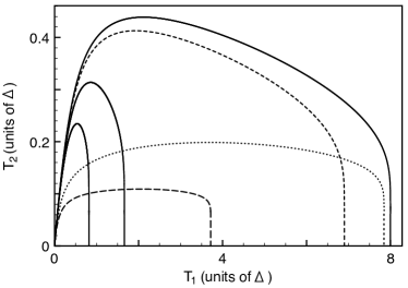
Figure 2: Entanglement region in the $(T_{1},T_{2})$ plane for $K_{1}=0$. The TLS steady state is entangled for temperatures below the drawn line. The solid lines correspond to $K_{2}=J_{2}$, $\xi=0$, and $J_{2}/J_{1}=5$, $10$ and $50$. The size of the entanglement region increases with $J_{2}$. For the dashed and dotted lines, the coupling parameters are $\xi=0$, and, respectively, $K_{2}=0.72J_{2}$ and $J_{2}=500J_{1}$, and $K_{2}=0.8J_{2}$ and $J_{2}=150J_{1}$. The short-dashed line is obtained for an Ohmic $\xi=0.01T_{1}/\Delta$ and for $K_{2}=J_{2}=50J_{1}$.

As an interesting example, we consider the case $\xi=0$ and $K_{1}=0$. This last condition means that the indirect interaction between the TLS is mediated only by bath $2$. With this value of $K_{1}$, the results discussed here hold also for the three bath setup depicted in Fig.1 when $T_{3}=T_{1}$. We find that there can be a low-temperature region, determined by $J_{2}/J_{1}$ and $K_{2}/J_{2}$, in which $\rho$ is entangled, see Fig.2. We remark that the line delimiting this entanglement region in the $(T_{1},T_{2})$ plane, is tangent to the equilibrium line $T_{1}=T_{2}$ for $T_{1},T_{2}\rightarrow 0$, and is essentially vertical at its other end for $T_{2}\ll\Delta$. These two behaviors come from the fact that the temperatures contribute to $\rho$ only via Boltzmann factors $\exp(-\Delta/T_{n})$.

Analytical results can be obtained by expanding the eigenvalue $\lambda_{-}$ to lowest order in these factors. It assumes negative values in the vicinity of $T_{1}=T_{2}=0$, for $|K_{2}|>J_{2}/\sqrt{2}$ and $J_{2}>J_{1}[\sqrt{2}|K_{2}|/J_{2}-1]^{-1}$. These requirements are the same in the Ohmic case discussed at end of IV.1, for which $\xi={\bar{\xi}}_{1}T_{1}+{\bar{\xi}}_{2}T_{2}$ vanishes in the limits $T_{1},T_{2}\rightarrow 0$. For given coupling parameters satisfying the above conditions, $\rho$ is not entangled if the temperatures $T_{1}$ and $T_{2}$ are too high. However, for $\xi=0$, the maximum possible value of $T_{1}$ is proportional to $\Delta J_{2}/J_{1}$ in the large $J_{2}$ limit, see Fig.2. Consequently, in this case, entangled states exist for any temperature $T_{1}$. For $T_{2}$, in contrast, our numerical results suggest that the steady state is always separable for $T_{2}$ greater than a value of about $0.567\Delta$. Entangled states can be observed close to this temperature in the limit of large $J_{2}$. For $\xi={\bar{\xi}}_{1}T_{1}+{\bar{\xi}}_{2}T_{2}$, $\rho$ is necessarily separable for $T_{1}$ higher than a temperature that diverges for ${\bar{\xi}}_{1}\rightarrow 0$.

IV.3.2 Requirements on the characteristics of the environment

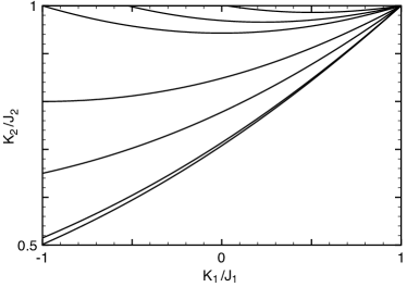
Figure 3: Region of the parameter plane $(K_{1}/J_{1},K_{2}/J_{2})$, $K_{2}>0$, where entangled steady states can be found, for $J_{2}/J_{1}=2.4$, $2.7$, $3$, $5$, $10$, $100$ and $1000$. The entanglement region is above the drawn line. Its size increases with $J_{2}$, to a maximum asymptotic value which is practically reached for $J_{2}=1000J_{1}$.

Stationary entanglement can also be obtained for $K_{1}\neq 0$. Since $\rho$ is obviously invariant under the bath permutation $(J_{1},K_{1})\leftrightarrow(J_{2},K_{2})$, it is enough to consider $J_{2}>J_{1}$. In this case, it can be shown that there exist entangled steady states in the vicinity of $T_{1}=T_{2}=0$ if

$$\left(J_{1}+J_{2}\right)^{2}-\left(K_{1}+K_{2}\right)^{2}-\left|K_{1}+K_{2}\right|\left|K_{2}-K_{1}\frac{J_{2}}{J_{1}}\right|<0.$$ (25)

This condition remains the same if the signs of both $K_{1}$ and $K_{2}$ are changed. Figure 3 shows, for $K_{2}>0$, the coupling parameter region where $\rho$ can be found entangled. The following interesting conclusions can be drawn from these results. There is a particular value of $J_{2}/J_{1}$ below which $\rho$ is separable. In other words, the couplings to the two heat baths must differ enough from each other in order to observe stationary entanglement. For given $J_{2}/J_{1}$ and $K_{1}/J_{1}$ such that entangled steady states exist, these states are obtained for $|K_{2}|/J_{2}$ not too far from $1$.

As mentioned above, the ratio $|K_{2}|/J_{2}$ depends essentially on the distance $d_{2}$ between the two points of bath $2$ where the TLS are connected. More precisely, it is determined by a dimensionless parameter ${\bar{d}}=\Delta d_{2}/v$ where $v$ is a characteristic field velocity of bath $2$. The ratio $|K_{2}|/J_{2}$ is small for large ${\bar{d}}$. This imposes limitations on $\Delta$ and on the temperature $T_{2}$ to obtain an entangled steady state. A distance $d_{2}$ of $1\mu$m and a low field velocity $v$ of $10^{3}$ m.s^-1, which is the order of magnitude of the sound velocity in solids, give a temperature of about $10$ mK, which is an experimentally accessible value. Another important characteristic of bath $2$ is its dimensionality $D$. For example, for a continuous free field, $K_{2}/J_{2}$ is equal to $\sin({\bar{d}})/{\bar{d}}$ for $D=3$, $J_{0}({\bar{d}})$ where $J_{0}$ is the zeroth order Bessel function of the first kind, for $D=2$, and $\cos({\bar{d}})$ for $D=1$. Thus, in this last case, stationary entanglement can be obtained for large distances $d_{2}$ and the limitations discussed above do not apply.

IV.3.3 Maximum attainable entanglement

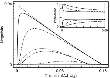
Figure 4: Negativity as a function of $T_{1}$ in units of $\Delta J_{1}/J_{2}$ for $K_{2}=J_{2}=100J_{1}$ (short-dashed line), $K_{2}=J_{2}=1000J_{1}$ (full line), $K_{2}=0.95J_{2}=9.5J_{1}$ (dash-dotted line) and $K_{2}=0.95J_{2}=95J_{1}$ (dashed line). The dotted lines correspond to the large $J_{2}$ approximation discussed in the text. The inset shows the populations of the ground and singlet states as functions of $T_{1}$ in units of $\Delta J_{1}/J_{2}$ for $K_{2}=0.95J_{2}=95J_{1}$, $K_{2}=J_{2}=100J_{1}$ and $K_{2}=J_{2}=1000J_{1}$. The two other populations are small. The other parameters are $\xi=0$, $K_{1}=0$ and $T_{2}=0.1\Delta$.

Finally, we present quantitative results for the entanglement of the steady state $\rho$. As a measure of entanglement, we use the negativity ${\cal N}(\rho)=(\|\rho^{\Gamma}\|_{1}-1)/2$ where $\|.\|_{1}$ denotes the trace norm ZHSL ; VW . Negativity ranges from $0$ for separable states to $1/2$ for maximally entangled states. Here, it is equal to $-\lambda_{-}$ when this eigenvalue is negative, and to $0$ otherwise. The maximum value of ${\cal N}$ that we have found, is reached for the coupling parameters $K_{1}=0$, $\xi=0$ and $J_{2}\gg J_{1}$, and the temperatures $T_{2}\ll\Delta$ and $T_{1}\gg\Delta$, see Fig.4. In this regime, the TLS steady state is given by

$$p_{1}=\sigma\left[(1+\theta)^{2}(1+2\theta)-\kappa^{2}\right] p_{2}=\sigma\theta(1+\theta)(1+2\theta)$$ ,

$$p_{4}=\sigma\theta^{2}(1+2\theta) c=-\sigma\kappa\theta$$ , (26)

where $\sigma=[(1+2\theta)^{3}-\kappa^{2}]^{-1}$, $\kappa=K_{2}/J_{2}$ and $\theta=(T_{1}/\Delta)(J_{1}/J_{2})$. For $|\kappa|\neq 1$, as $\theta$ increases from zero to infinity, the ground state population $p_{1}$ decreases from $1$ to $1/4$, $p_{2}=p_{3}$ and $p_{4}$ increases from $0$ to $1/4$, and $|c|$ increases from zero to a maximum and then decays back to zero. The low $\theta$ behavior is very different for $|\kappa|=1$. In this case, $c$ is finite in the limit $\theta\rightarrow 0$. For $K_{2}=\pm J_{2}$ and a temperature $\Delta\ll T_{1}\ll\Delta J_{2}/J_{1}$, we find $\rho=(2/3)|+\rangle_{1}{{}_{1}\langle+|}\otimes|+\rangle_{2}{{}_{2}\langle+|}+(1/3)|\psi^{\mp}\rangle\langle\psi^{\mp}|$ with the Bell states $|\psi^{\mp}\rangle$ given by (17), and a negativity ${\cal N}=(\sqrt{5}-2)/6\simeq 0.04$. The same entangled state can be reached for $K_{1}\neq 0$, as it will be clear from the discussion below. Our numerical results suggest that finite values of ${\cal N}$ correspond generally to states $\rho$ such that essentially only the ground state and one of the Bell states (17) are populated, see inset of Fig.4.

To better understand the above results, it is interesting to consider the rates discussed after (17). For $T_{2}\ll\Delta$ and $T_{1}\gg\Delta$, the rates of the upward transitions $|1\rangle\rightarrow|\psi^{\pm}\rangle$ and $|\psi^{\pm}\rangle\rightarrow|4\rangle$ are $r_{up}^{\pm}=(J_{1}\pm K_{1})T_{1}/\Delta$, and that of the downward transitions $|4\rangle\rightarrow|\psi^{\pm}\rangle$ and $|\psi^{\pm}\rangle\rightarrow|1\rangle$ are $J_{2}\pm K_{2}+r_{up}^{\pm}$. For $K_{2}=J_{2}$ and $T_{1}\ll\Delta J_{2}/J_{1}$, the rate of $|4\rangle\rightarrow|\psi^{-}\rangle$ and $|\psi^{-}\rangle\rightarrow|1\rangle$ is equal to $r_{up}^{-}$, whereas that of $|4\rangle\rightarrow|\psi^{+}\rangle$ and $|\psi^{+}\rangle\rightarrow|1\rangle$ is $2J_{2}\gg r_{up}^{\pm}$. Consequently, the states $|4\rangle$ and $|\psi^{+}\rangle$ are essentially not populated, and the transition rate from the state $|\psi^{-}\rangle$ to the ground state $|1\rangle$ is effectively twice that of the reverse transition, leading to a factor of two between the two corresponding populations. The situation is similar fo $K_{2}=-J_{2}$. If $|K_{2}|$ is too far from $J_{2}$ or if $T_{1}$ is too high, the values of the different rates are comparable and so are the populations of the states $|1\rangle$, $|\psi^{\pm}\rangle$ and $|4\rangle$, and hence $\rho$ is separable.

V Conclusion

In summary, we have studied a system of two independent TLS weakly coupled to a stationary non-equilibrium environment. Considering first a general open system, we have determined their steady state. Without specifiying any further the surroundings of the TLS, it can be shown that their steady state is uncorrelated if their splitting energies are different from each other. Moreover, the state of each TLS is the same wether or not the other TLS is present. Consequently, in this case, a finite strength of the coupling to the environment is required to possibly generate stationary TLS entanglement. In the opposite case of identical splitting energies, on the contrary, stationary correlations between the TLS can exist for extremely weak coupling to the environment.

To determine wether these correlations can be quantum, we have considered the case of an environment consisting of several bosonic heat baths at different temperatures. We have shown that, for TLS coupled similarly to two baths, there are temperatures and coupling parameters for which the TLS steady state is entangled. An important requirement is that, for at least one bath, the points to which the TLS are connected must be close enough to each other. However, this condition can be relaxed when one of the bath is one-dimensional. In this case, the TLS can be as far apart as we like. There are also requirements on the baths temperatures. Essentially, one of them must be sufficiently low, of the order of the TLS splitting energy. Depending on the characteristics of the coupling, the other temperature can be unlimited.

We have found a parameter regime where the TLS steady state is a statistical mixture of the product ground state and of the entangled singlet state with weights 2/3 and 1/3, respectively. This mixed state is entangled and the corresponding negativity is about 0.04 which is the largest value we have obtained. Interestingly, this regime can be fully understood in terms of Fermi golden rule transitions between appropriate states. To conclude, our results show that a relatively simple non-equilibrium environment can lead to stationary entanglement of two TLS, but certainly do not exhaust all the possible effects of stationary non-equilibrium surroundings on quantum correlations. Larger entanglement of independent TLS, as measured by negativity for instance, may be achievable with other environments or for TLS coupled differently to the environment. Further studies in these directions would be of interest.

Appendix A Special uncorrelated states

In this appendix, our purpose is to show that, for some special cases, the solution of (10) is of the form $u_{kl}=p_{k}\delta_{kl}$. This is the case if the sums

$$\sum_{k^{\prime}}\gamma_{kl,k^{\prime}k^{\prime}}(i0^{+})p_{k^{\prime}}=\pi\sum_{A,B,k^{\prime}}P_{A}\langle A|h_{kk^{\prime}}|B\rangle\langle B|h_{k^{\prime}l}|A\rangle\\ \times\left[\left(p_{k}+p_{l}-2\frac{P_{B}}{P_{A}}p_{k^{\prime}}\right)\delta(\omega_{AB}-\omega_{k^{\prime}k})+\frac{i}{\pi}\frac{p_{l}-p_{k}}{\omega_{AB}-\omega_{k^{\prime}k}}\right]\\$$ (27)

vanish for $k$ and $l$ such that $\epsilon_{k}=\epsilon_{l}$.

For an environment in thermal equilibrium, i.e., $P_{A}\propto\exp(-E_{A}/T)$ where $T$ is its temperature, $u_{kl}\propto\exp(-\epsilon_{k}/T)\delta_{kl}$ satisfies (10) since, in the sums (LABEL:sum), $p_{k}=p_{l}$ and $P_{B}p_{k^{\prime}}/P_{A}p_{k}=\exp[-(\omega_{BA}+\omega_{k^{\prime}k})/T]$. This proof applies to any system ${\cal S}$.

We now consider the case of zero splitting energy $\Delta_{2}$ and of an environment ${\cal E}$ that consists of heat baths at different temperatures $T_{n}$. First, the populations $p_{k}$ obtained in section III.2 ensure the vanishing of (LABEL:sum) for $k=l$. For $k\neq l$, we start by showing that ${\tilde{\gamma}}_{2}^{+}={\tilde{\gamma}}_{2}^{-}$ which implies $p_{1}=p_{2}$ and $p_{3}=p_{4}$, see (13). The difference of these rates reads as

$${\tilde{\gamma}}_{2}^{+}-{\tilde{\gamma}}_{2}^{-}=2\pi\sum_{A,B}(P_{A}-P_{B})|\langle B|w_{2}|A\rangle|^{2}\delta(\omega_{AB}).$$ (28)

For the kind of environment considered, $H_{\cal E}=\sum_{n}H_{{\cal E}n}$ and hence its eigenstates and eigenenergies can be written as $|A\rangle=\prod_{n}|A^{(n)}\rangle$ and $E_{A}=\sum_{n}E_{A^{(n)}}$. The populations $P_{A}$ factorise as $P_{A}\propto\prod_{n}\exp(-E_{A^{(n)}}/T_{n})$. The TLS are coupled to each bath thus $w_{2}=\sum_{n}w_{2n}$. Consequently, the difference (28) satisfies

$${\tilde{\gamma}}_{2}^{+}-{\tilde{\gamma}}_{2}^{-}\propto\sum_{n}\sum_{A^{(n)},B^{(n)}}|\langle B^{(n)}|w_{2n}|A^{(n)}\rangle|^{2}\\ \times\left(e^{-E_{A^{(n)}}/T_{n}}-e^{-E_{B^{(n)}}/T_{n}}\right)\delta(E_{A^{(n)}}-E_{B^{(n)}})$$ (29)

and hence vanishes. For $\Delta_{2}=0$, the sum (LABEL:sum) must be zero for $(k,l)=(1,2)$, $(2,1)$, $(3,4)$ and $(4,3)$. For these cases, the equalities $p_{1}=p_{2}$ and $p_{3}=p_{4}$, shown above, lead to

$$\sum_{k^{\prime}}\gamma_{kl,k^{\prime}k^{\prime}}(i0^{+})p_{k^{\prime}}=2\pi\sum_{A,B,k^{\prime}}\langle A|h_{kk^{\prime}}|B\rangle\langle B|h_{k^{\prime}l}|A\rangle\\ \times\left(p_{k}P_{A}-P_{B}p_{k^{\prime}}\right)\delta(\omega_{AB}-\omega_{k^{\prime}k}).$$ (30)

For the Hamiltonian (1), $h_{14}=h_{23}=0$ and hence the only terms that contribute to the above sum are such that $p_{k^{\prime}}=p_{k}$ and $\omega_{kk^{\prime}}=0$. Thus, it vanishes for the same reasons as (28) does.

For $\Delta_{1}=\Delta_{2}=0$, the sum (LABEL:sum) must be zero for any $(k,l)$. In this case, for an environment that consists of heat baths, $u_{kl}=\delta_{kl}/4$ satisfies (10) since $\sum_{k^{\prime}}\gamma_{kl,k^{\prime}k^{\prime}}(i0^{+})=0$.

References

- (1) R.F. Werner, Phys. Rev. A 40, 4277 (1989).
- (2) J.S. Bell, Physics (Long Island City, NY) 1, 195 (1964).
- (3) K. Zyczkowski, P. Horodecki, A. Sanpera and M. Lewenstein, Phys. Rev. A 58, 883 (1998).
- (4) M.O. Terra Cunha, New J. Phys 9, 237 (2007).
- (5) T. Yu and J. H. Eberly, Phys. Rev. Lett. 93, 140404 (2004).
- (6) L. Jacóbczyk and A. Jamróz, Phys. Lett. A 333, 35 (2004).
- (7) T. Yu and J. H. Eberly, Phys. Rev. B 66, 193306 (2002).
- (8) P. J. Dodd and J. J. Halliwell, Phys. Rev. A 69, 052105 (2004).
- (9) D. Braun, Phys. Rev. Lett. 89, 277901 (2002).
- (10) L. Jakóbczyk, J.Phys. A: Math. Gen. 35, 6383 (2002).
- (11) F. Benatti, R. Floreanini and M. Piani, Phys. Rev. Lett. 91, 070402 (2003).
- (12) D. P. S. McCutcheon, A. Nazir, S. Bose and A. J. Fisher, Phys. Rev. A 80, 022337 (2009).
- (13) P. Zanardi and M. Rasetti, Phys. Rev. Lett. 79, 3306 (1997).
- (14) L. Hartmann, W. Dür and H.-J. Briegel, Phys. Rev. A 74, 052304 (2006).
- (15) L. D. Contreras-Pulido and R. Aguado, Phys. Rev. B 77, 155420 (2008).
- (16) M.B. Plenio and S.F. Huelga, Phys. Rev. Lett. 88, 197901 (2002).
- (17) F. Kheirandish, S. J. Akhtarshenas and H. Mohammadi, Eur. Phys. J. D 57, 129 (2010).
- (18) Ö. Çakir, A. A. Klyachko and A. S. Shumovsky, Phys. Rev. A 71, 034303 (2005).
- (19) U. Weiss, Quantum dissipative systems (World Scientific, Singapore, 1993).
- (20) C. Cohen-Tannoudji, J. Dupont-Roc and G. Grynberg, Processus d’interaction entre photons et atomes (CNRS Editions, Paris, 1988).
- (21) S. Camalet, Eur. Phys. J. B 61, 193 (2008).
- (22) R.H. Lehmberg, Phys. Rev. A 2, 883 (1970).
- (23) A.J. Leggett, S. Chakravarty, A.T. Dorsey, M.P.A Fisher, A. Garg and W. Zwerger, Rev. Mod. Phys. 59, 1 (1987).
- (24) A. Peres, Phys. Rev. Lett. 77, 1413 (1996).
- (25) M. Horodecki, P. Horodecki and R. Horodecki, Phys. Lett. A 223, 1 (1996).
- (26) G. Vidal and R.F. Werner, Phys. Rev. A 65, 032314 (2002).