On Star Formation Rates and Star Formation Histories of Galaxies out to $z\sim 3$

Abstract

We compare multi-wavelength star formation rate (SFR) indicators out to $z\sim 3$ in the GOODS-South field. Our analysis uniquely combines $U$-to-8$\mu$m photometry from FIREWORKS, MIPS 24 $\mu$m and PACS 70, 100, and 160 $\mu$m photometry from the PEP survey, and $H\alpha$ spectroscopy from the SINS survey. We describe a set of conversions that lead to a continuity across SFR indicators. A luminosity-independent conversion from 24 $\mu$m to total infrared luminosity yields estimates of $L_{IR}$ that are in the median consistent with the $L_{IR}$ derived from PACS photometry, albeit with significant scatter. Dust correction methods perform well at low to intermediate levels of star formation. They fail to recover the total amount of star formation in systems with large $SFR_{IR}/SFR_{UV}$ ratios, typically occuring at the highest SFRs ($SFR_{UV+IR}\gtrsim 100\ M_{\sun}/yr$) and redshifts ($z\gtrsim 2.5$) probed. Finally, we confirm that $H\alpha$-based SFRs at $1.5<z<2.6$ are consistent with $SFR_{SED}$ and $SFR_{UV+IR}$ provided extra attenuation towards HII regions is taken into account ($A_{V,neb}=A_{V,continuum}/0.44$). With the cross-calibrated SFR indicators in hand, we perform a consistency check on the star formation histories inferred from SED modeling. We compare the observed SFR-M relations and mass functions at a range of redshifts to equivalents that are computed by evolving lower redshift galaxies backwards in time. We find evidence for underestimated stellar ages when no stringent constraints on formation epoch are applied in SED modeling. We demonstrate how resolved SED modeling, or alternatively deep UV data, may help to overcome this bias. The age bias is most severe for galaxies with young stellar populations, and reduces towards older systems. Finally, our analysis suggests that SFHs typically vary on timescales that are long (at least several 100 Myr) compared to the galaxies’ dynamical time.

1. Introduction

Determining when the stars were formed is one of the main goals in galaxy evolution. Two widely adopted approaches to this question are to measure the assembled stellar mass at various lookback times (see, for the local universe, Cole et al. 2001; Bell et al. 2003, at intermediate redshifts Bundy et al. 2006; Borch et al. 2006; Pozzetti et al. 2007; Vergani et al. 2008, and out to $z\sim 5$ Dickinson et al. 2003; Fontana et al. 2003, 2004, 2006; Drory et al. 2004, 2005; Elsner et al. 2008; Pérez-González et al. 2008; Marchesini et al. 2009), or to quantify the rate of on-going star formation over cosmic time (Madau et al. 1996; Lilly et al. 1996; Steidel et al. 1999; Giavalisco et al. 2004; Schiminovich et al. 2005; Bouwens et al. 2007, 2010). While the latter should in principle integrate up to the former, modulo stellar mass loss, it is currently heavily debated whether or not the data, or rather the physical quantities estimated from them, satisfy this continuity equation (Hopkins & Beacom 2006; Reddy & Steidel 2009).

The relation between the instantaneous star formation rate (SFR) and stellar mass of individual galaxies sheds light on how (in bursts or gradually) and where (in galaxies of what mass) the star-forming activity took place (Noeske et al. 2007; Elbaz et al. 2007; Daddi et al. 2007a). At a given mass, observations show a rapidly increasing SFR with redshift (e.g., Lilly et al. 1996; Cowie et al. 1996; Bell et al. 2005), whereas the models predict an increase in growth rate that is significantly slower (Davé 2008; Damen et al. 2009).

Both issues urge us to critically investigate the assumptions made in translating fluxes and colors to an estimate of the SFR. Especially the presence of dust greatly impacts the interpretation of multi-wavelength data. The SFR indicators considered in this paper come in two flavors: either the rate of unobscured and obscured star formation is summed ($SFR_{UV+IR}$ in this paper), or the rate of unobscured star formation is scaled up by a dust correction factor ($SFR_{\rm SED}$, $SFR_{UV,corr}$ and $SFR_{H\alpha}$ in this paper). The former requires knowledge of the total infrared (IR) luminosity ($L_{IR}$) emitted in the rest-frame 8-1000 $\mu$m range by dust that was heated by young stars, often extrapolated from the observed 24 $\mu$m photometry. The latter requires knowledge of how the observed colors break down in intrinsic colors of the stellar population and dust reddening, which both are model dependent.

Here, we exploit the wealth of multi-wavelength data in the GOODS-South field, including HST/ACS, HST/WFC3, VLT/ISAAC, Spitzer/IRAC, Spitzer/MIPS 24 $\mu$m, and Herschel/PACS 70 - 160 $\mu$m imaging, as well as VLT/SINFONI $H\alpha$ spectroscopy to calibrate SFR indicators of galaxies out to $z\sim 3$. This work lays the basis for Wuyts et al. (2011b), where we analyze galaxy morphologies as a function of position in the SFR-Mass diagram. In order to carry out such a systematic study of the entire galaxy population over a large range of masses and SFRs, establishing a continuity across SFR indicators is essential. This is obviously of more general use as well. Doing so, our analysis places constraints on the distribution of dust within these galaxies, and on their star formation histories (SFHs). In addition, we exploit the inferred SFRs and SFHs to test whether galaxy populations at different lookback times satisfy a continuity equation.

We present a brief overview of the data used in Section 2. Next, we make the case for a luminosity-independent conversion to $L_{IR}$ in Section 3. SFRs derived by summing a UV and IR contribution are contrasted to SED modeled SFRs and dust-corrected UV SFRs in Section 4, and to $H\alpha$-derived SFRs in Section 5. Section 6 discusses the consistency of inferred SFHs, and introduces resolved SED modeling as a means to better characterize the age of the bulk of the stars in a galaxy. Finally, we summarize our results in Section 7.

Throughout this paper, we quote magnitudes in the AB system, and adopt the following cosmological parameters: $(\Omega_{M},\Omega_{\Lambda},h)=(0.3,0.7,0.7)$.

2. Sample and Observations

2.1. FIREWORKS $K_{s}$-selected Catalog

The backbone of this work is the $K_{s}$-selected FIREWORKS catalog sampling the $U$-to-8$\mu$m regime with 16 passbands ($K_{s,lim}=24.3,\ 5\sigma$; Wuyts et al. 2008, hereafter W08). Initially, we focus on the 1333 galaxies in the redshift range $0<z<3$ that were significantly detected ($>3\sigma$) at 24$\mu$m. Redshifts are spectroscopic for 69% of the sample below $z<1.5$, and for 27% above $z>1.5$. For the remaining sources, we derived high-quality photometric redshifts using EAZY (Brammer et al. 2008). The median and normalized median absolute deviation in $\Delta z/(1+z)$ are $(-0.002;\ 0.025)$ at $z<1.5$ and $(-0.003;\ 0.044)$ at $z>1.5$.

2.2. PEP GOODS-S Survey

The GOODS-South field has been observed with the Photodetector Array Camera and Spectrometer (PACS, Poglitsch et al. 2010) onboard the Herschel Space Observatory as part of the PACS Extragalactic Survey (PEP, Lutz et al. 2011). With $5\sigma$ depths for prior extraction of 1.8 mJy, 1.9 mJy and 3.3 mJy at 70 $\mu$m, 100 $\mu$m, and 160 $\mu$m respectively, it is the only PEP field to be imaged at 70 $\mu$m, and a factor 2.5 - 4.5 deeper than the other PEP blank fields at 100 $\mu$m and 160 $\mu$m. These observed bands sample rest-frame wavelengths close to the peak of IR emission of galaxies in our redshift range of interest. For an in depth description of the observations, data reduction and catalog building, we defer to Berta et al. (2010) and Lutz et al. (2011). Briefly, the PACS photometry used in this paper was obtained by PSF-fitting using the positions of MIPS 24 $\mu$m detected sources from Magnelli et al. (2009) as prior. Adopting this positional prior reduces the effects of confusion, and is justified by the relative depths of the MIPS and PACS imaging.

2.3. SINS GOODS-S Sample

The SINS survey (e.g., Förster Schreiber et al. 2006, 2009; Genzel et al. 2006, 2008) is a VLT/SINFONI GTO program targeting 80 high-redshift star-forming galaxies, providing integral-field emission line maps and integrated fluxes without slit losses. We focus on the subset of 25 SINS galaxies located in the GOODS-South field with H$\alpha$ observations spanning a redshift range $1.5<z<2.6$, and a range in stellar mass from $5.1\times 10^{9}M_{\sun}$ to $1.4\times 10^{11}M_{\sun}$. Their location in the SFR versus mass diagram is representative for that of the underlying population of star-forming galaxies at similar redshift.

3. SFRs from adding UV and IR emission

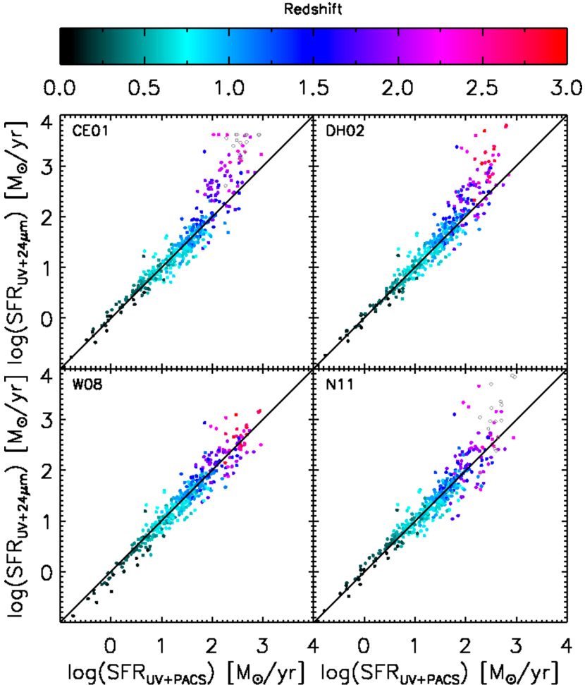
Figure 1.— Star formation rates of galaxies at $0<z<3$ based on UV plus 24 $\mu$m emission versus UV plus PACS emission. The IR part of the SFR is proportional to the total IR luminosity $L_{IR}$, which was derived monochromatically using conversions and template sets from CE01, DH02, W08, and N11. Adopting the locally calibrated luminosity-dependent recipes from CE01 and DH02 to convert observed 24 $\mu$m fluxes to $L_{IR}$ leads to overpredicted SFRs at the high-redshift and high-SFR end. For N11, these cases are limited to redshifts above $z>2.5$, where the 24 $\mu$m filter enters $\lambda_{rest}<6\ \mu$m, and the CE01/N11 templates lack a physically realistic calibration (open gray circles).

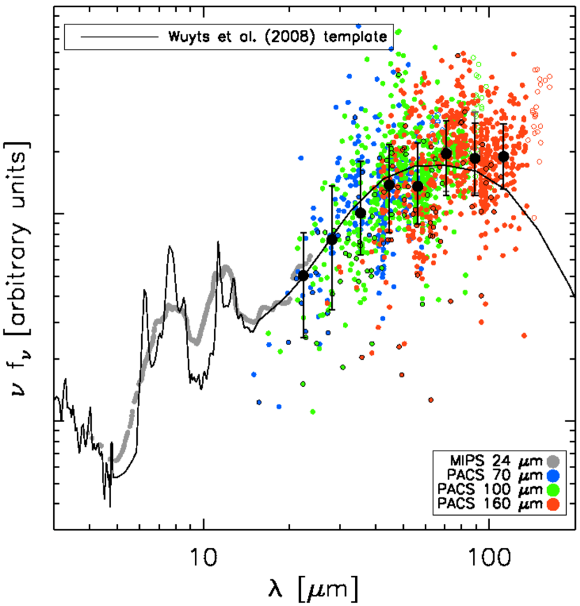
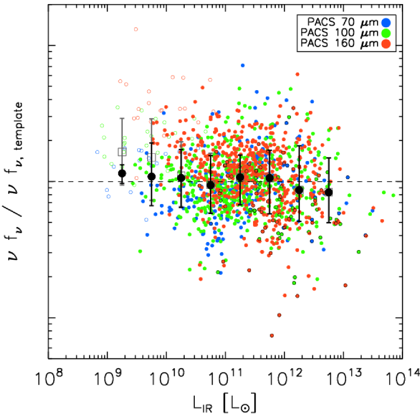
Figure 2.— Top: Spectral energy distribution template by Wuyts et al. (2008), with the observed photometry of PACS-detected galaxies at $z<3$ in the GOODS-South field overplotted at the respective rest-frame wavelengths. For every galaxy, a uniform scaling is applied to its $24-160\ \mu$m photometry so as to normalize the observed 24 $\mu$m flux (gray) to the template (black) convolved by the MIPS passband. Large black symbols indicate the binned median and standard deviation of the scaled PACS photometry, matching the template, albeit with a significant (0.25 dex) scatter. Small black circles mark sources with an X-ray luminosity above $10^{42}\ erg\ s^{-1}$. Bottom: Residual from the Wuyts et al. (2008) template as function of inferred total IR luminosity. Large empty boxes and filled circles indicate the binned median, with and without galaxies at $z<0.2$ respectively. Excluding the most nearby galaxies (small empty circles), only a marginal trend with IR luminosity remains.

In this Section, we analyze SFR indicators based on adding the unobscured and obscured star formation, traced by the UV and IR emission respectively. With the advent of PACS/Herschel, the emission at or near the IR peak can now be probed directly out to high redshift to unprecedented depths (see, e.g., Nordon et al. 2010; Elbaz et al. 2010). Combining PACS and SPIRE data, Elbaz et al. (2010) found that the total IR luminosity ($L_{IR}\equiv L(8-1000\ \mu m)$) can be derived reliably from a single PACS band. We will therefore restrict ourselves to such monochromatic conversions to $L_{IR}$ in this paper.

The depth of PACS imaging in the GOODS-South field (2.0 mJy at 160 $\mu$m, 3$\sigma$) is among the deepest of all IR lookback surveys. In most other fields, the derivation of $L_{IR}$ or $SFR_{UV+IR}$ from PACS photometry has to rely on stacking analyses to reach the same depths. In order to preserve information on an individual object level, IR luminosities for all but the brightest galaxies must then be derived from MIPS 24 $\mu$m. Here, we exploit the deep mid- and far-IR data in GOODS-South to test for internal consistency between them.

We consider four conversion recipes. The conversions by Chary & Elbaz (2001, hereafter CE01) and Dale & Helou (2002, hereafter DH02) rely on locally calibrated template libraries, where the template adopted from the library depends on the galaxy’s luminosity (generally yielding larger conversion factors for more luminous galaxies at a given redshift). Studying PACS observations in GOODS-North, Nordon et al. (2010) argued for enhanced emission of polycyclic aromatic hydrocarbons (PAHs) in $z\sim 2$ galaxies relative to local galaxy SEDs of the same $L_{IR}$. Accounting for this, Nordon et al. (2011, hereafter N11) formulate a recalibration of the CE01 library for the $1.5<z<2.5$ regime (below $z<1.5$, the original CE01 conversion is used). Specifically, these authors find little to no luminosity dependence of the rest-frame 20-60 $\mu$m SED shape for the $L_{IR}\gtrsim 10^{11}\ L_{\sun}$ regime probed. In the mid-infrared, their conversion has a luminosity dependence, but such that the ratio $\nu L_{\nu}(rest-8\mu m)/L_{IR}$ at a given redshift and luminosity is larger than that from CE01. Finally, Wuyts et al. (2008) introduced a luminosity-independent conversion based on a single template, which was motivated by MIPS 24 $\mu$m, 70 $\mu$m, and 160 $\mu$m stacking results by Papovich et al. (2007). This template was constructed by averaging the logarithm of DH02 templates with the parametrization $\alpha$ of the intensity of the interstellar radiation field in the range $1<\alpha<2.5$ in steps of 0.0625. In terms of local analogs, its mid- to far-infrared SED shape is more reminiscent of M82 than of Arp220.

In Figure 1, we present a comparison of $SFR_{UV+24\mu m}$ to $SFR_{UV+PACS}$ for PACS-detected galaxies out to $z=3$, for each of the above $L_{IR}$ conversion recipes. In each case, the total SFR is derived following Kennicutt (1998):

$$SFR_{UV+IR}\ [M_{\sun}\ yr^{-1}]=1.09\times 10^{-10}\ (L_{IR}+3.3L_{2800})/L_{\sun}$$ (1)

where the relative scaling of the UV and IR contribution is based on calibrations in the local universe, and the overall scaling factor assumes a Chabrier (2003) IMF. The rest-frame luminosity $L_{2800}\equiv\nu L_{\nu}(2800\AA)$ was computed with EAZY from the best-fitting SED, itself a superposition of the 6 EAZY principle-component templates. Only at the lowest redshifts ($z<0.3$), rest-frame 2800Å falls blueward of the available photometry. For $SFR_{UV+PACS}$, we use the longest wavelength PACS band that had a significant ($>3\sigma$) detection. The color-coding indicates the redshift of the galaxies. It is a well-known fact that galaxies that are highly actively star-forming are more common at larger lookback times. The lower end of the SFR distribution at a given redshift is simply determined by the flux limit of our sample.

At $z\ll 2$ and $SFR<100\ M_{\sun}/yr$, we find little difference between the PACS and 24 $\mu$m-based estimates, irrespective of the conversion recipe used. However, above $z\gtrsim 2$ and for SFRs above $100\ M_{\sun}/yr$, the 24 $\mu$m-based estimates using the locally calibrated CE01 and DH02 conversions are clearly overestimated with respect to those based on PACS photometry. At $1.5<z<2.5$, no such systematic bias is present in the case of the W08 and N11 conversions. These results imply that, rather than having mid- to far-IR SEDs as local ULIRGs, ULIRGs at $z\sim 2$ are better characterized as scaled-up versions of local LIRGs, which are colder than nearby ULIRGs. This finding is in agreement with recent results by Nordon et al. (2010), Elbaz et al. (2010), Muzzin et al. (2010), and Symeonidis et al. (2011).

We point out that any variation in $\nu L_{\nu}(24\mu m)/L_{IR}$, where $L_{\nu}(24\mu m)$ refers to the specific luminosity probed by the observed 24 $\mu$m band, translates superlinearly to variations in $L_{IR}(24\ \mu m)/L_{IR}(160\ \mu m)$ when applying a luminosity-dependent conversion. This leads to a somewhat increased scatter around unity in the $L_{IR}(24\ \mu m)/L_{IR}(160\ \mu m)$ ratio of $1.5<z<2.5$ galaxies for N11 ($\sim 0.4$ dex) compared to W08 ($\sim 0.3$ dex), since the scatter in $\nu L_{\nu}(24\mu m)/L_{IR}$ at a given luminosity is large compared to any systematic variation of $\nu L_{\nu}(24\mu m)/L_{IR}$ over the luminosity range probed. More importantly, the luminosity-independent conversion by W08 has the advantage of being applicable also above $z>2.5$, where N11 shows more systematic outliers. This is at least in part due to the fact that the 24 $\mu$m band starts entering the $\lambda_{rest}\lesssim 6\ \mu$m regime where the CE01 templates lack a physically realistic calibration.

In order to address the uncertainties involved in converting 24 $\mu$m to $L_{IR}$ in more detail, we present the W08 template in Figure 2. Overplotted, we show the IR photometry of $0<z<3$ galaxies that are individually detected ($>3\sigma$) in at least one PACS band. Their 24 $\mu$m flux is normalized to match the template flux within the passband at the respective redshift, but their 24 $\mu$m - PACS colors are left as observed. Black filled circles and error bars mark the median and central 68th percentiles for PACS-detected galaxies at $0.2<z<3$, respectively. Gray empty circles and error bars illustrate small changes when including the lowest redshift ($z<0.2$) sources. Although a significant scatter (0.25 dex in $\Delta\log\nu f_{\nu}$) is notable, the observations are in the median consistent with the W08 template. Moreover, Figure 2b demonstrates that the residuals from the template do not strongly correlate with the $L_{IR}$ derived from the respective PACS band, especially when excluding local ($z<0.2$) galaxies, that dominate the lowest luminosities ($10^{9}\ L_{\sun}<L_{IR}<10^{10}\ L_{\sun}$). In other words, we observe a spread in 24 $\mu$m - PACS colors, even at a given redshift, but this spread does not seem to correlate strongly with galaxy luminosity. As a consequence of the observed flux limits, different luminosity bins in Figure 2b will naturally be populated by galaxies of a different redshift distribution. This could potentially mask some luminosity dependence present within a narrow redshift slice. Including also observations at 16 $\mu$m, N11 investigate this by probing the rest-frame 8 $\mu$m luminosity in bins of both $L_{IR}$ and redshift, finding a dependence on both albeit with significant scatter. While not capturing these physics, the W08 SED can be considered as an effective template offering a simple and robust conversion from observed 24 $\mu$m photometry to $L_{IR}$. The 7.7 $\mu$m PAH strength may increase with redshift relative to $L_{IR}$ (see N11), but for the purpose of converting MIPS 24 $\mu$m to $L_{IR}$, it is sufficient that its strength in the template is appropriate for $z\sim 2$, where this feature is sampled by the 24 $\mu$m passband. Given that the scatter in $\nu L_{\nu}(24\mu m)/L_{IR}$ is large compared to any variation with luminosity, not accounting for a luminosity dependence has the compensating advantage that deviations in $\nu L_{\nu}(24\mu m)$ at a given luminosity do not translate nonlinearly to $L_{IR}(24\mu m)$. Another parameter potentially contributing to the scatter observed in Figure 2b, is the dust temperature. More specifically, variations in the dust temperature from galaxy to galaxy would express themselves as deviations from a unique SED shape, and hence a source of scatter in Figure 2b. Magdis et al. (2010) recently reported a wide range of dust temperatures in high-redshift ULIRGs. For an in depth discussion of the relation between dust temperatures and other characteristics of high-redshift galaxies (such as SFR and mass), we defer the reader to Magnelli et al. (in prep). In the Appendix, we briefly discuss possible contributions by Active Galactic Nuclei (AGN), but argue that they do not affect the above results for the ensemble of PACS-detected galaxies. For a first exploration of AGN in the context of PACS observations, we refer the reader to Shao et al. (2010).

In the above analysis, we focussed on PACS detections only. While half of the 24 $\mu$m sources in GOODS-South are not detected at any PACS wavelength, the PACS sample is matched quite well to the 24 $\mu$m depth of other, shallower fields. For example, 90% of the galaxies brighter than the 24 $\mu$m detection threshold of COSMOS are PACS-detected in GOODS-South. This implies that the conversion described in this section can safely be applied to translate the COSMOS 24 $\mu$m photometry to $L_{IR}$. We briefly explored how the median SED shape changes when going beyond the PACS detection threshold by means of stacking. We computed the median stacked fluxes in bins of rest-frame wavelength now including all sources detected at 24 $\mu$m. Stacking was performed after scaling the PACS postage stamps by the same factor used to normalize the 24 $\mu$m flux of the corresponding object to the W08 template. Postage stamps of PACS-undetected sources were cut out of residual maps from which all individually detected sources were subtracted. We find that the blue side of the far-IR bump ($20\ \mu m<\lambda_{rest}<60\ \mu m$) is somewhat more depressed, by $\sim 0.15$ dex with respect to the W08 template to which the 24 $\mu$m flux was normalized. However, the amplitude of the peak in IR emission, where the bulk of the energy emitted at 8 - 1000 $\mu$m comes from, is well matched by the template. The 8 - 1000 $\mu$m integral over the DH02 or CE01 template that best fits the shape of the median stacked SED deviates by merely a percent from that of the W08 template, making the latter an acceptable basis for deriving $L_{IR}$ for our full 24 $\mu$m-detected sample.

We conclude that a continuity between 24 $\mu$m and far-infrared based SFR indicators can be obtained out to $z=3$, albeit with significant scatter. The good median performance of the W08 conversion in the light of new Herschel observations is encouraging for recent studies in which it was applied (Franx et al. 2008; Wuyts et al. 2009b; Damen et al. 2009; Kajisawa et al. 2010).

4. SFRs from SED Modeling and dust-corrected UV emission

In GOODS-South, not only the PACS but also the MIPS depth (0.02 mJy at 24 $\mu$m, 5$\sigma$) is one of the deepest available. Consequently, in studies that exploit larger areas to reduce cosmic variance effects, one will be limited by the shallower MIPS imaging of other fields. Other SFR tracers than IR-based methods are therefore indispensable.

4.1. Cross-calibration to $SFR_{UV+IR}$

Modeling of broad-band SEDs with stellar population synthesis models is one of the most commonly used approaches, as it is a more generally accessible means to derive SFRs (among other stellar population properties) for galaxies over a wide range of redshifts and types. It can also be extended to fainter galaxies with lower SFRs.

We investigate the performance of this technique, which is essentially a dust correction method, by comparing it to $SFR_{UV+IR}$ for galaxies with a PACS and/or MIPS detection. The $L_{IR}$ that enters the computation of $SFR_{UV+IR}$ was calculated using the W08 template and the longest wavelength IR band that had a significant detection. We adopt default assumptions regarding SED modeling. Briefly, exponentially declining SFHs, also known as $\tau$ models, were constructed from the Bruzual & Charlot (2003, hereafter BC03) stellar population synthesis models, and fitted to the $U$-to-8 $\mu$m FIREWORKS SEDs using the fitting code FAST (Kriek et al. 2009). We are aware that increasing star formation histories have recently been proposed as more appropriate for galaxy evolution at early times ($z\gtrsim 3$, Renzini et al. 2009; Maraston et al. 2010; Papovich et al. 2011), and explore this option further in Section 6.2.2. For now, we restrict the analysis of our $0<z<3$ sample to default $\tau$ models whose wide use in the literature makes it worthwhile testing their performance in light of the new IR constraints. As throughout the paper, we adopt a Chabrier (2003) IMF, and we assume solar metallicity. We required the time since the onset of star formation to be at least 50 Myr, and not exceeding the age of the universe at the epoch of observation. We experimented with minimum e-folding times varying between 10 Myr and 10 Gyr. The fitting procedure minimizes the $\chi^{2}$ statistic taking discrete steps of 0.1 dex in age and $\tau$ within the allowed range. We allow the galaxies to be attenuated within a range of visual extinctions $0<A_{V}<4$, in steps of 0.1 mag, assuming a uniform foreground screen geometry, and with the reddening following the Calzetti et al. (2000) law. We refer to the instantaneous SFR of the best-fit model as $SFR_{SED}$.

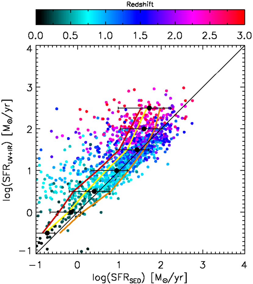
Figure 3.— The SFRs of IR-detected galaxies at $0<z<3$ based on adding the unobscured (UV) and re-emitted (IR) radiation of newly formed stars versus SFRs from stellar population modeling of observed optical-to-mid-IR SEDs. Here, SFR_SED was derived using BC03 models with exponentially declining SFHs (with $\log(\tau_{min})=8.5$). For modest levels of star formation ($SFR\lesssim 50\ M_{\sun}\ yr^{-1}$), both SFR indicators agree well in the median (large black circles, with error bars indicating the central 68th percentile). At higher SFRs, which become increasingly more common toward higher redshift, the SED-modeled SFR systematically underpredicts that inferred from UV + IR. Red and yellow curves illustrate the median relation when adopting less stringent constraints ($\log(\tau_{min})=7$ and 7.5 respectively) on the minimum e-folding time. The orange line marks the median relation when allowing very long ($\log(\tau_{min})=10$) e-folding times only.

We find the best correspondence to $SFR_{UV+IR}$ when forcing the e-folding time to be larger than $\log\tau_{min}=8.5$. The plotted points in Figure 3 correspond to this set of boundary conditions. The majority of galaxies, at low to intermediate ($SFR_{UV+IR}\lesssim 50\ M_{\sun}/yr$) SFRs line up along a ridge line which coincides with the one-to-one relation. A tail toward lower SED-modeled SFRs is present, and contains more than 50% of the galaxies at the high SFR (and high redshift) end. When allowing shorter e-folding times, we find these are often preferred in a least-squares sense, but leave a systematic offset in SFR in comparison to measurements of $SFR_{UV+IR}$. The red and yellow line in Figure 3 indicate the median trend for $\log\tau_{min}=7.0$ and 7.5 respectively. It thus seems that e-folding timescales of at least several 100 Myr give results that are more consistent with UV+IR based estimates than more rapidly declining histories. In Section 6.2, we will describe independent evidence in this direction, based on the implausibly young ages inferred from fits with small $\tau$ values. Changing $\log(\tau_{min})$ from 8.5 to 9 leads to a similar performance in the comparison to $SFR_{UV+IR}$. However, when allowing very long e-folding times only ($\log(\tau_{min})=10$), $SFR_{SED}$ becomes an overestimate at intermediate star formation levels (see orange curve in Figure 3). Overall, we recommend $\log(\tau_{min})=8.5$, for its effectiveness at reproducing the low to intermediate SFRs while not overly restricting the allowed range of SFHs.

To contrast this timescale of $\sim 300$ Myr for variations in star formation activity with another characteristic timescale of the galaxies in our sample, we computed the dynamical time $t_{dyn}=\sqrt{\frac{R^{3}}{2GM}}$ of the 27% of galaxies that are covered by the HST/WFC3 Early Release Science program. Here, we measured the effective radius $R$ by fitting Sersic models to the $H$-band surface brightness distribution using GALFIT v3.0 (Peng et al. 2010). We find typical $\tau/t_{dyn}$ ratios of order $\sim 50$, with large variations from 10 to 100 and up. This implies that most star formation happened in a relatively stable mode over long timescales, as opposed to a single short burst taking place on a dynamical time. Similar conclusions were drawn by Genzel et al. (2010), who pushed the study of the Schmidt-Kennicutt law (Schmidt 1959; Kennicutt 1998) and the Elmegreen-Silk relationship (Elmegreen 1997; Silk 1997) for normal star-forming galaxies to $z\sim 1-3$.

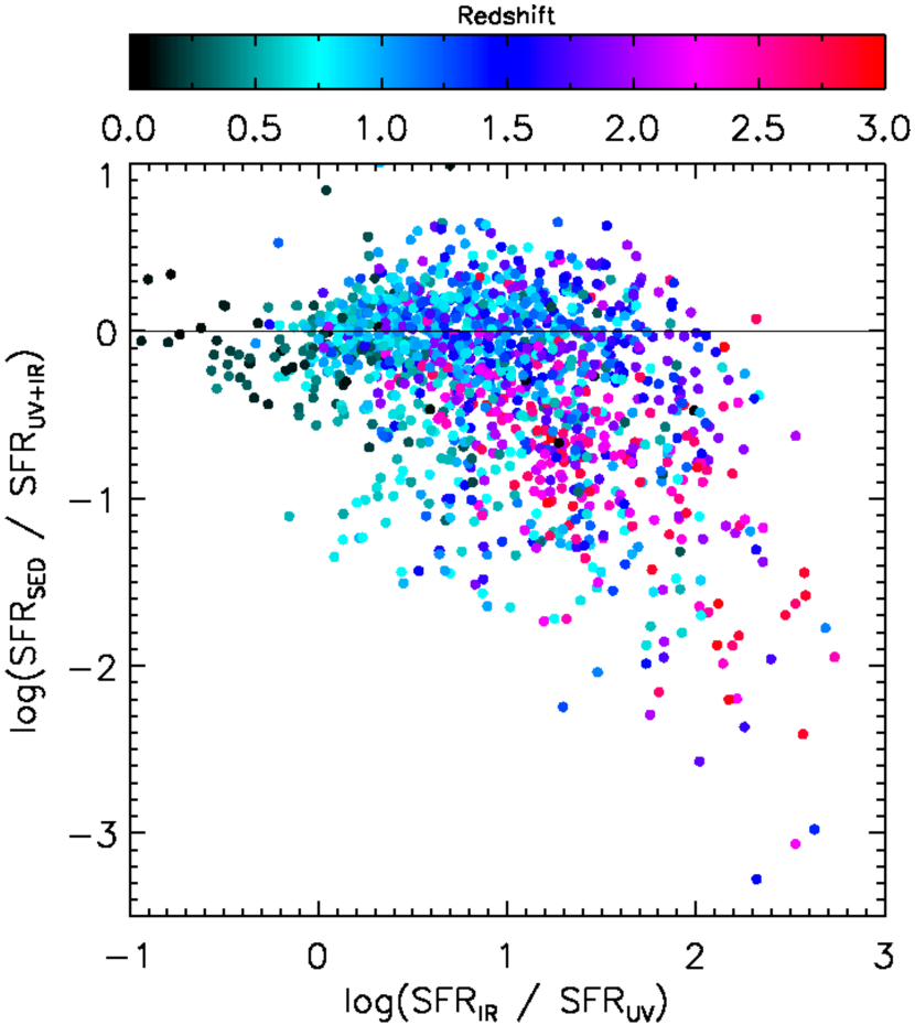
Figure 4.— Ratio between SFR_SED and SFR_UV+IR as function of relative fraction of radiation from young stars that is re-processed by dust versus escaping without attenuation. The underprediction of the total amount of star formation by SFR_SED (i.e., a dust correction method) is most severe for galaxies that have the largest $SFR_{IR}/SFR_{UV}$ ratio. These conditions are more prevalent in vigorously star-forming systems, as found more commonly at high redshift. Saturation of reddening as an extinction tracer due to a patchy dust distribution is responsible for this effect.

Despite the good overall correspondence between the SFR indicators, the tail of systematic underestimates by $SFR_{SED}$, reaching an order of magnitude at the largest $SFR_{UV+IR}\sim 300\ M_{\sun}/yr$ (predominantly galaxies at $z\gtrsim 2.5$) remains worrisome. Such a trend at the high-SFR end was previously signaled by Santini et al. (2009) on the basis of pre-Herschel data sets. Figure 4 sheds light on its origin. The deviation from a one-to-one relation between $SFR_{UV+IR}$ and $SFR_{SED}$ is a clear function of the relative ratio of emission from young stars that is re-processed by dust versus escaping unhindered as UV light. The diagram illustrates that particularly when the unattenuated UV emission reveals only a few percent of the total star formation (i.e., when the dust correction factor is very large), a simplistic dust correction method based on a uniform foreground screen does not account properly for optical depth effects. The reason is that information on the dust correction factor is not directly embedded in the galaxy’s SED. It is the reddening of the spectral slope that is directly traced, but only translates linearly to extinction when the obscuring material has the configuration of a foreground screen. In case of patchy dust obscuration, or dust that is mixed with the emitting sources, reddening saturates as a tracer of extinction. In the case of selective extinction towards young star-forming regions, the resulting underestimate of the SFR can be even more pronounced (Poggianti et al. 2001; Wuyts et al. 2009a). The same effect is seen in local ULIRGs (Goldader et al. 2002) and starburst galaxies (e.g., Förster Schreiber 2001 and references therein) that lie above the well-known IRX-$\beta$ relation (Meurer et al. 1999), and in hydrodynamic simulations of high-redshift (merging) galaxies (Wuyts et al. 2009a, Fig. 10). Our conclusion confirms the recent results by Reddy et al. (2010), who find that galaxies with large IR luminosities ($L>10^{12}\ \L_{\sun}$) at $z\sim 2$ also lie above the IRX-$\beta$ relation, unlike more modestly star-forming galaxies at the same epoch.

4.2. Single-color SFRs for Star-forming $z\sim 2$ Galaxies

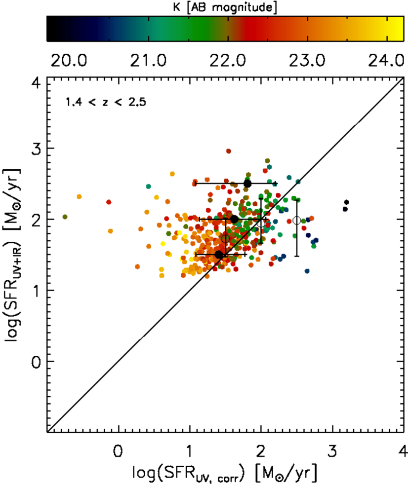
Figure 5.— The SFRs of IR-detected galaxies at $1.4<z<2.5$ based on adding the unobscured (UV) and re-emitted (IR) radiation of newly formed stars versus the Daddi et al. (2007) dust correction method which relies solely on the observed $B-z$ color. Large filled and open symbols indicate the median in bins of $SFR_{UV+IR}$ and $SFR_{UV,corr}$ respectively. Whereas the two methods yield consistent results at modest SFR ($\lesssim 50\ M_{\sun}\ yr^{-1}$) levels, the dust correction method fails to recover the total amount of star formation at the highest SFR_UV+IR bin. Note that inferred systematic offsets are dependent on the K-band limit of the sample.

Daddi et al. (2004; 2007a) introduced an observed color criterion to dust-correct UV SFRs of BzK galaxies at $1.4<z<2.5$. Since it is based on observed-frame, rather than rest-frame photometry, it has the limitation of only being applicable to the redshift range for which it was designed. On the other hand, it has the advantage of being more easily accessible, as it only requires $B$ and $z$ photometry (and $K$ in order to select the high-redshift galaxies in the first place). Furthermore, it has been argued that the use of such a limited wavelength range avoids dilution of the information on the rate of star formation by degeneracies with other stellar population parameters. It is therefore useful to address the performance of the Daddi et al. (2007a) criterion in light of the $SFR_{UV+IR}$ calibrations (Section 3), that are now motivated by the new Herschel/PEP photometry.

Figure 5 presents a comparison of $SFR_{UV+IR}$ to the single-color dust correction method by Daddi et al. (2007). We plot all galaxies with an IR detection (i.e., for which $SFR_{UV+IR}$ is not an upper limit), most of which satisfy the BzK criterion. Despite the limited range in redshift and SFR probed, a similar trend emerges as seen for the SED modeling (Section 4.1). While at intermediate $SFR_{UV+IR}$, the two SFR indicators agree well, the dust correction method fails to recover the total amount of star formation at the largest $SFR_{UV+IR}$. We note that, when binning in $SFR_{UV,corr}$ (i.e., the SFR indicator to be tested) instead of $SFR_{UV+IR}$ (our reference SFR indicator), the median $SFR_{UV+IR}$ of the highest $SFR_{UV,corr}$ bin actually lies below the one-to-one relation (large open circles). The fact that the median binned relation depends on the axis that is binned reflects a significant scatter in the relation between the UV+IR and dust-corrected SFR. The absence of a tight relation may stem from variations in the dust distribution from galaxy to galaxy. The color-coding in Figure 5 furthermore indicates that the scatter is not random, but that instead the relation between the two SFR indicators is a function of $K$-band magnitude. This illustrates that the offset with respect to $SFR_{UV+IR}$ depends on the properties of the galaxy sample. E.g., stacking $K$-bright ($K<22$) galaxies in bins of $SFR_{UV,corr}$ Nordon et al. (2010) found an excess of 0.3 dex for dust-corrected UV SFRs.

We conclude that we do not find any evidence that a single color dust correction method would be more precise than SFRs from modeling of the full $U$-to-8 $\mu$m SED. Both dust correction methods perform equally well in the redshift range $1.4<z<2.5$ where they overlap, with similar biases for the dusty, most rapidly star-forming systems. Resolved SED modeling on the scale of the patchiness of the dust distribution may help to overcome the saturation of reddening as an extinction tracer when IR data are not available (see Section 6.4, and in more detail Wuyts et al. in prep).

4.3. Dependence on Stellar Population Synthesis Models

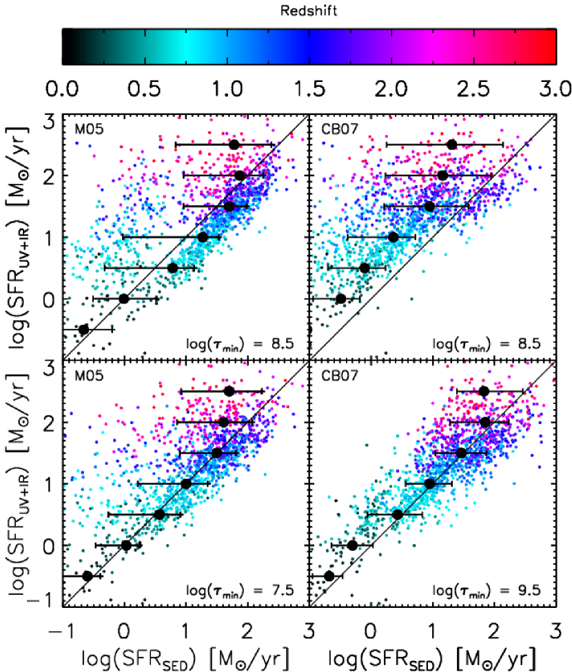
Figure 6.— Idem as Figure 3, but using different stellar population synthesis codes (M05 and CB07 instead of BC03) to derive SFR_SED. In the top panels, identical constraints on the SFH (specifically the minimum allowed e-folding time $\tau_{min}$) as for Figure 3 were used. This leads to SED-modeled SFRs that are more discrepant from SFR_UV+IR than SFR_SED,BC03. By tuning $\tau_{min}$ (bottom panels), a correspondence to SFR_UV+IR of similar quality can be obtained. In all cases, the saturation of reddening as extinction tracer in dusty, star-bursting (high-redshift) galaxies leads to systematic underestimates of SFR by the SED modeling method.

Even under identical assumptions on SFH and dust reddening, differences between stellar population synthesis codes give rise to systematic uncertainties in the determination of stellar population properties. The impact of the treatment of certain stellar evolutionary phases, such as the thermally pulsating AGB phase, on the estimated stellar mass and age of (high-z) galaxies has been discussed extensively elsewhere (see, e.g., Maraston 2005, hereafter M05; Maraston et al. 2006; Wuyts et al. 2007). In Figure 6, we focus on the implications for SFR recipes. The top two panels compare $SFR_{UV+IR}$ to $SFR_{SED}$ as derived with M05 and Charlot & Bruzual (2007, hereafter CB07) models. We adopted the same restriction of a minimum e-folding time of $\log\tau_{min}=8.5$ that provided the best agreement for BC03 models. Similar to the BC03 comparison in Figure 3, the SED modeled SFRs lead to underestimates at the high $SFR_{UV+IR}$ end. However, at intermediate and low SFRs the behavior looks markedly different, especially for the CB07 models that lead to consistently lower estimates of the SFR by $\sim 0.4$ dex. Adjusting a single parameter $\tau_{min}$ in our SED modeling recipe, it is possible to calibrate both $SFR_{SED,\ M05}$ and $SFR_{SED,\ CB07}$ such that they produce an equally good match to $SFR_{UV+IR}$ as $SFR_{SED,\ BC03}$. In other words, our cross-calibration of SFR indicators cannot discriminate between different stellar population synthesis models. We find, however, that BC03, M05 and CB07 models require different constraints on the minimum e-folding time ($\log\tau_{min}=8.5$, 7.5, and 9.5 respectively) in order to optimally match the UV+IR based indicator.

Figure 6 demonstrates that the SED fitting results based on M05 and CB07 models show qualitative differences despite the fact that both contain an updated implementation of the TP-AGB phase, leading to increased rest-frame $K$-band fluxes and lower stellar mass estimates. The two stellar population synthesis models differ in at least two aspects. First, the boost in rest-frame $K$-band light due to TP-AGB stars occurs at earlier times for CB07 (around $\log age\sim 8.5$) compared to M05 (around $\log age\sim 9$). Second, the optical (rest-frame $U-V$) colors by CB07 are identical to those of BC03, whereas they are redder by nearly 0.2 mag in the M05 models for most of the ages considered. This stems from the use of different stellar tracks that do (in the case of CB07) or do not (for M05) include convective overshooting (see Maraston et al. 2006; Fagotto et al. 1994 for the Padova stellar tracks used by CB07; Cassisi et al. 1997 for the Frascati stellar tracks used by M05). Together, these differences lead to best-fit solutions that in the case of M05 correspond to younger, dustier and more actively star-forming systems than inferred from BC03 fits, while CB07 fits yield lower SFRs and $A_{V}$, and older ages. As we will discuss in Section 6, the stellar ages derived from BC03 models without stringent constraints on formation redshift or e-folding time tend to be implausibly young. This problem may therefore be even more pressing when considering M05 fits. Finally, we note that for both M05 and CB07 fits, solutions with ages for which the TP-AGB contribution is maximal, seem to be avoided. The apparent bimodality in the upper left panel of Figure 6 is a reflection of this bimodality in estimated ages. Along similar lines, Kriek et al. (2010) recently reported that, for their sample of post-starburst galaxies at $0.7<z<2.0$, a low contribution from TP-AGB stars was demanded in order to reproduce their spectral energy distributions.

To conclude, we find that, in common for all stellar population models considered, underestimates of the SFR for the dusty, most actively star-forming galaxies, that are abundantly present at high redshift, are intrinsic to any dust correction method assuming a uniform foreground screen. SED modeling recipes can be tuned to reproduce the level of star formation in galaxies with more modest $SFR_{UV+IR}$.

4.4. Dependence on Extinction Curve

So far, we always assumed the Calzetti et al. (2000) law for the wavelength dependence of the attenuation. Although this law is widely used in the high-redshift literature, reddening laws are known to vary, at least in the local universe, due to variations in dust composition and dust size distribution. Dust grains can grow to larger sizes as the density of the gas to which they are mixed increases, leading to a larger ratio of visual extinction to reddening $R_{V}\equiv A_{V}/E(B-V)$ (Maiolino & Natta 2002 and references therein). At larger lookback times as well, such variations in environment may cause the extinction curve to vary between galaxies of different type. Along these lines, Reddy et al. (2010) recently argued that young $z\sim 2$ galaxies with ages $<100$ Myr may follow an extinction curve that is different from Calzetti, and instead more SMC-like.

Here, we briefly consider how our results would change when adopting the SMC reddening law from Prévot et al. (1984) and Bouchet et al. (1985), which increases more steeply towards short wavelengths compared to the relatively gray Calzetti law. Naturally, when adopting the SMC law, less dust (i.e., a smaller $A_{V}$) is needed to reproduce the observed UV spectral slope. Furthermore, it is interesting to note that without imposing an ad hoc constraint on the minimum $\tau$, the best-fit $\tau$ and age distribution are less skewed towards short $\tau$ and young ages. For the same weak constraints on $\tau$ ($\log\tau_{min}>7$), we find that the underestimate of $SFR_{SED}$ with respect to $SFR_{UV+IR}$ is reduced to 0 - 0.2 dex at low $SFR_{UV+IR}\lesssim 20\ M_{\sun}/yr$ when adopting the SMC law. At high SFRs on the other hand, the discrepancy becomes worse. In terms of $\chi^{2}$, half of the low $SFR_{UV+IR}<20\ M_{\sun}/yr$ systems are better fit with a SMC law than a Calzetti law, while above $SFR_{UV+IR}>20\ M_{\sun}/yr$ this fraction drops to 20%.

From the comparison to $SFR_{UV+IR}$ and the relative distribution of $\chi^{2}$ values, we thus conclude that our results are at least qualitatively consistent with a scenario where steeper extinction curves are appropriate for lower SFR systems. Physically, this may stem from a dust grain distribution that is biased to small sizes in these environments that are typically of lower gas density. For simplicity, consistency with previous work, and because a good SFR calibration can be obtained provided an appropriate $\tau_{min}$ (see Section 4.1), we will proceed in this paper to only use the Calzetti law. More direct probes of the extinction curve at high redshift, and its variation with galaxy luminosity, age, and/or SFR are desired.

5. SFRs from $H\alpha$

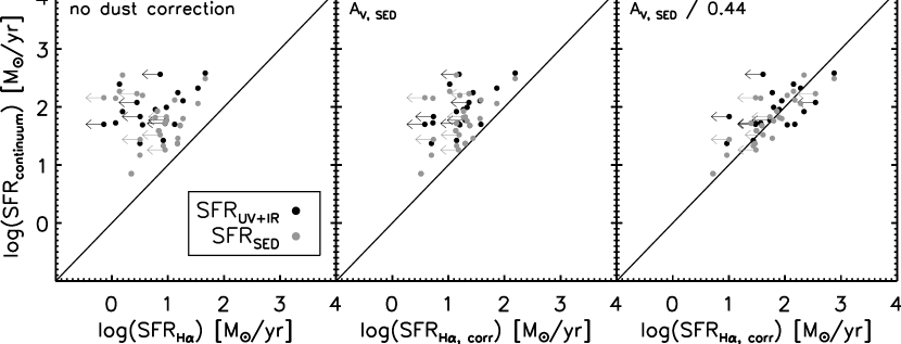
Figure 7.— SFRs of SINS galaxies at $1.5<z<2.6$ as derived from continuum measurements (UV+IR and SED modeling methods) compared to the star formation rate as inferred from the $H\alpha$ line luminosity under various assumptions about its extinction. In the absence of a dust correction, or when simply applying the dust correction as inferred from broad-band SED modeling, the $H\alpha$-based SFR is clearly underestimated with respect to other indicators. Adopting the locally calibrated extra attenuation towards HII regions compared to the continuum yields a better correspondence to the other SFR indicators.

We established self-consistent recipes for SFRs based on UV + IR and SED modeling. Now, we extend the cross-calibration of SFR indicators to measurements of the $H\alpha$ line luminosity, as obtained by SINFONI on VLT as part of the SINS survey (Förster Schreiber et al. 2009). The benefit of using integral field spectroscopy is the absence of slit losses, which complicate the absolute calibration of total $H\alpha$ luminosities from slit-based measurements (e.g., Erb et al. 2006; Reddy et al. 2010). This sample comprises 25 star-forming galaxies in the GOODS-South field spread over the redshift range $1.5<z<2.6$, out which 19 are significantly ($>3\sigma$) detected in $H\alpha$. SINFONI exposure times ranged from 1 to 8.5 hours. Tests on partial data sets of the longest exposed targets indicate that possible sensitivity-driven flux losses for the shortest exposed objects are $\sim 30$%. 19 out of 25 sources are significantly detected in the MIPS 24 $\mu$m band, and for 9 of those we extracted PACS fluxes with $S/N>3$. We derived monochromatic $L_{IR}$ using the longest wavelength IR band that has a significant detection. In addition to $SFR_{UV+IR}$ values for the IR-detected sources, we also compute SED modeled SFRs for all 25 galaxies in this sample. The two continuum-based estimators are contrasted to the line-based measurement $SFR_{H\alpha}$ in Figure 7.

The H$\alpha$ fluxes were converted to star formation rates $SFR_{H\alpha}$ following the prescription of Kennicutt (1998), which assumes case B recombination, corrected to a Chabrier (2003) IMF. Not unexpectedly, the rates are severely underestimated when no dust correction is applied (left panel). Using the Calzetti et al. (2000) reddening law, the visual extinction $A_{V}$ translates to the extinction at the rest-wavelength of H$\alpha$ as $A_{H\alpha}=0.82A_{V}$. When adopting the visual extinction as inferred from broad-band SED modeling $A_{V,\ SED}$ (middle panel), we find the offsets in SFR to be reduced, but still amounting to underestimates of 0.55 dex.

Indeed, it was found by Förster Schreiber et al. (2009) that the SINS data are consistent with roughly twice higher attenuation towards the HII regions relative to the bulk of the stars. Pioneering measurements of the Balmer decrement $H\alpha/H\beta$ in high-z galaxies seem to confirm the increased extinction towards HII regions, albeit with a significant galaxy-to-galaxy scatter in the precise degree of differential extinction (Yoshikawa et al. 2010; Muzzin et al. 2010; Buschkamp et al. in prep).

In nearby galaxies, it has long been established that HII regions are often associated with dustier regions than the bulk of the stellar populations across galaxies (Calzetti et al. 1994, 2000; Cid-Fernandes et al. 2005). Studying a sample of low-redshift star-forming and starburst galaxies, Calzetti et al. (2000) formulated the empirical calibration $A_{V,neb}=A_{V,SED}/0.44$ where $A_{V,neb}$ and $A_{V,SED}$ refer to the visual extinction towards the nebular regions and the stellar continuum respectively.

Here, the offset in the middle panel of Figure 7 reflects this need to take into account differential extinction. Applying the local calibration to our high-redshift sample (right panel of Figure 7), we find the H$\alpha$-based SFR to line up well with estimates based on UV+IR and SED modeling. We measure a median $\Delta\log SFR=\log SFR_{continuum}-\log SFR_{H\alpha}$ of 0.08, with a 0.33 dex scatter. We verified that our analysis leads to the same conclusion when deriving $A_{V,SED}$ using M05 models. Furthermore, the 3 objects in our sample that are X-ray detected, among which object ID6202 whose broad H$\alpha$ line profile suggests the presence of AGN activity and/or shocks, do not deviate from the remaining galaxies in our sample, implying that contributions to the H$\alpha$ luminosity by non-stellar processes do not dominate the observed trend.

Using SFR indicators from UV to IR wavelengths, we verified the findings on differential extinction by Förster Schreiber et al. (2009), which are also consistent with recent work by Onodera et al. (2010) and Mancini et al. (2011). In contrast, Reddy et al. (2010) found that such an extra attenuation correction towards HII regions may not be necessary. This may be due to observational effects (e.g., uncertain slit loss corrections), but differences between the intrinsic properties of the galaxy samples could play a role as well. The galaxies studied by Reddy et al. (2010) typically have lower stellar masses. Their extinction may differ due to different dust properties or distributions.

6. Life Paths through the SFR versus Mass Diagram: a Consistency Check

With the above calibrated ’ladder of SFR indicators’ and SED modeling recipes in hand, we now perform a galaxy population study, linking progenitors and descendants in the SFR versus mass diagram over a range of redshifts, and testing for consistency. We detail how observed populations at high redshift are compared to the expected populations inferred from observations at lower redshift in Section 6.1. In Section 6.2, we carry out this methodology multiple times, varying only the constraints on the galaxies’ SFH. Here, we make the case for underestimated galaxy ages as a significant contributor to the observed discrepancies. After addressing merging as another potential contributor (Section 6.3), we return to the issue of constraining galaxy ages in Section 6.4, arguing for an extended wavelength baseline, or spatially resolved SED modeling as avenues for improvement.

6.1. Methodology

If we ignore merging, a galaxy with a mass $M_{obs}$ in stars at the epoch of observation can be considered as one unit since its onset of star formation at time $t_{form}$, and built up its stellar content following

$$M_{obs}=\int_{t_{form}}^{t_{obs}}\!SFR(t-t_{form})f_{loss}(t_{obs}-t)\,\mathrm{d}t.$$ (2)

Here, the fraction $f_{loss}(t)$ accounts for stellar mass loss. This fraction of mass remaining in stars first declines rapidly once the first supernovae go off, then decreases more gradually by winds from AGB stars, reaching $\sim 0.6$ after 1 Gyr, and eventually levels off at $\sim 0.5$ for a Chabrier IMF (BC03).

As age will be an important parameter in our analysis, it is useful to point out that two definitions of galaxy age are frequently used in the literature; one being the time since the onset of star formation:

$$age=t_{obs}-t_{form},$$ (3)

and the other being a measure of the age of the bulk of the stars:

$$age_{w}=\int_{t_{form}}^{t_{obs}}\!SFR(t-t_{form})(t_{obs}-t)\,\mathrm{d}t\ /$$

$$\int_{t_{form}}^{t_{obs}}\!SFR(t-t_{form})\,\mathrm{d}t.$$ (4)

For exponentially declining SFHs, $age_{w}$ ranges between $0.5\times age$ ($\tau=\infty$) and $1\times age$ ($\tau=0$). Throughout this paper, when referring to $age_{w}$, we will explicitly state ’SFR-weighted age’.

Given equation 2, a particular functional form (in our case parametrized by $\tau$) for the star formation history $SFR(t)$ translates to a unique path $SFR(M)$ of the galaxy in the SFR versus mass diagram. Consequently, the constraints on $M_{obs}$, $\tau$, and $SFR_{obs}$ allow us to determine the location of each galaxy’s progenitor in the SFR-M diagram at any point earlier in time. For galaxies with a PACS and/or MIPS detection, we apply the IR constraints to the SED modeling by searching for the minimum $\chi^{2}$ solution within a 0.1 dex range around $SFR_{UV+IR}$. This approach reduces the degrees of freedom by one. In addition, it avoids the underestimates by $SFR_{SED}$ at the high-SFR end (see Section 4.1). For galaxies that lack a far- or mid-IR detection, we simply use the SED modeling performed without constraints on the SFR.

We then compare the galaxy population observed at $1<z<2$ to that expected at that epoch from tracing the $0<z<1$ population back in time. Likewise, we confront the observed $2<z<3$ population to that backtraced from $1<z<2$, and the $3<z<4$ population to that inferred from galaxies at $2<z<3$. Under our premise that galaxies satisfy a continuity equation over cosmic time, both the location of the main sequence of star formation, and how densely it is populated should match. The presence of any discrepancies could hint at ill-characterized SFHs, breaking of number conservation by merging, or cosmic variance leading to one redshift interval being under- or overdense with respect to the other.

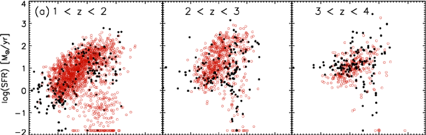
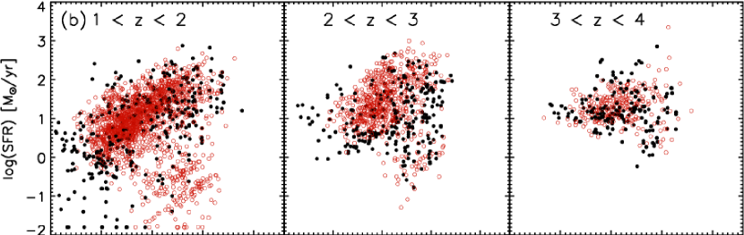
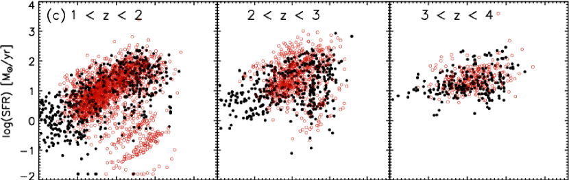
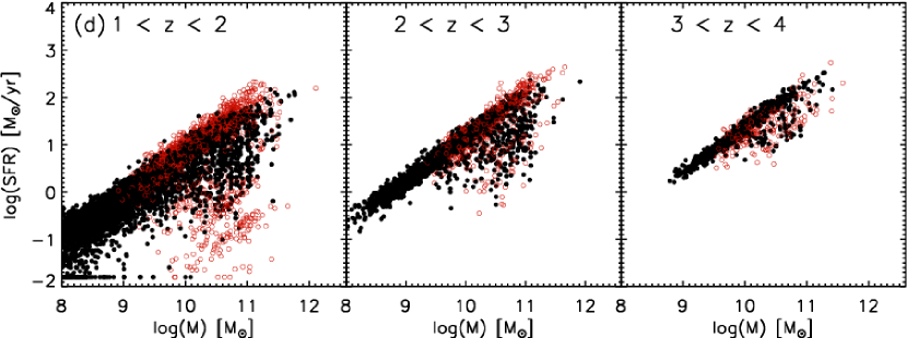
Figure 8.— Observed (red) SFR versus stellar mass diagram in three redshift bins, compared to the distribution and population expected for the same volume from tracing galaxies in the previous redshift bin back in time (black). The following constraints were applied in modeling the SEDs with BC03 templates: (a) $\tau$ models with $\log(\tau_{min})=7.5$, (b) $\tau$ models with $\log(\tau_{min})=8.5$, (c) delayed $\tau$ models with $\log(\tau_{min})=8.5$, (d) delayed $\tau$ models with $\log(\tau_{min})=8.5$ and all galaxies being maximally old. While occupying a similar region in the SFR versus mass diagram as the observed galaxies, the backtraced population is undernumerous at all redshifts in cases (a) to (c), suggesting an overall underestimate of formation redshifts, especially when no stringent constraints on e-folding time and/or age are imposed.

6.2. Tracing Galaxies back in Time

6.2.1 $\tau$ Models

We first perform the above described galaxy population analysis adopting exponentially declining SFHs with a large range of allowed e-folding timescales ($\tau>30$ Myr). In Figure 8a, we contrast the observed SFR-M relation (red) to that inferred from the SED modeled SFHs of galaxies in the previous redshift bin (black). The black and red symbols were plotted in a random order, in order to preserve information on the relative abundance of the two populations, even in crowded regions of the diagram. At all redshifts, the backtraced model matches the observed main sequence of star formation reasonably well in terms of zeropoint, slope, and scatter. In particular, even though $\tau$ models by definition do not allow for increasing SFRs, the upwards shift of the main sequence from $z=0$ to $z=3$ is captured by the model. As is empirically well established, galaxies with lower specific star formation rates exist alongside normal star-forming galaxies at least out to $z\sim 3$ (see, e.g., Labbé et al. 2005; Kriek et al. 2006). Their relative abundance is an increasing function of galaxy mass, and declines with increasing redshift (Fontana et al. 2009). We note that, while these quiescent systems are abundantly present at $1<z<2$, they are missing from the backtraced population computed for that redshift bin. Galaxies with similarly low specific star formation are present in our $0<z<1$ sample. This suggests that we are not merely missing the descendants of $1<z<2$ quiescent galaxies due to the smaller volume probed at $0<z<1$. In general, it is the case that the backtraced number densities, both on and off the main sequence, are at all redshifts lower than those directly observed.

This result is quantitatively better appreciated when we collapse the SFR-M diagram along the SFR axis, resulting in the mass functions plotted in Figure 9a. Here, the solid lines represent the observed mass function at different redshifts. In agreement with Marchesini et al. (2009), whose analysis was partly based on the same data set, we observe fairly little evolution in number density at the high-mass ($>10^{11}\ M_{\sun}$) end, compared to a steeper build-up of stellar mass with cosmic time in the intermediate ($\sim 10^{10}\ M_{\sun}$) regime. We did not correct the observed mass functions for incompleteness. Instead, we apply the $K=24.3$ observed magnitude limit of the FIREWORKS catalog to the galaxies that were evolved back in time, leading to the dashed curves in Figure 9a. This approach allows for a fair comparison as long as galaxies’ higher-z progenitors have fainter observed $K$-band magnitudes than their descendants at the epoch of observation.

Figure 9a clearly shows that the backtraced population, as based on SED modeling with $\tau$ models with a large freedom in $\tau$, is underpopulated. The underestimate of the number densities increases with decreasing stellar mass, becoming dramatic at intermediate masses, particularly for the lower redshift bins, where it exceeds an order of magnitude. As we will see in Section 6.3, such large differences in number density are unlikely to result from merging of galaxies alone, a process that we ignored so far in our analysis. An underdensity of the GOODS-South field in the $0<z<1$ interval (Wolf et al. 2003) may contribute to the offset seen between the observed and backtraced $1<z<2$ population. However, the same trend is seen at all redshifts. This cannot be due solely to field-to-field variations unless each redshift bin is underdense relative to the one above. Moreover, the magnitude of the offsets seems incompatible with field-to-field variations. Following the methodology of Somerville et al. (2004), the expected uncertainty due to cosmic variance on the number density of $\log M>10.5$ galaxies at $0<z<1$, $1<z<2$, $2<z<3$, and $3<z<4$ as derived from the GOODS-South field is 34, 24, 26 and 32% respectively, much smaller than the discrepancies between the observed and backtraced populations in Figure 9a. The most straightforward interpretation is therefore that the SED modeled stellar populations are biased towards young stellar ages. Given an underestimated age, we would infer the stellar mass of a galaxy to be built up relatively recently. Or in other words, as we trace this galaxy back in time, its stellar mass would decrease too rapidly, leading to a lower formation redshift at which the galaxy drops out of the backtraced sample. The origin of such age underestimates lies most plausibly in the fact that younger stellar populations outshine any underlying old population in the integrated SED, especially at the shorter wavelengths. Because of this outshining effect, any deviation from the simple SFH and foreground dust distribution assumed makes it impossible to correctly recover the true SFR-weighted age (Wuyts et al. 2009a; Maraston et al. 2010).

Somewhat earlier formation epochs are obtained when requiring longer e-folding timescales of $\tau>300$ Myr. Since this also provided a better agreement between SFR indicators (Section 4.1), we adopt this value of $\tau_{min}$ in the remainder of our analysis. In the median, the SFR-weighted age of the galaxies in our sample then increases by 0.15 dex. The high-mass end of the observed and backtraced mass functions now show a good agreement (Figure 9b). At lower masses, the offsets remain present, although reduced by a few 0.1 dex. The mass dependence of the offsets may imply that age underestimates are more of a concern for low- to intermediate-mass galaxies than for the most massive (often older) systems.

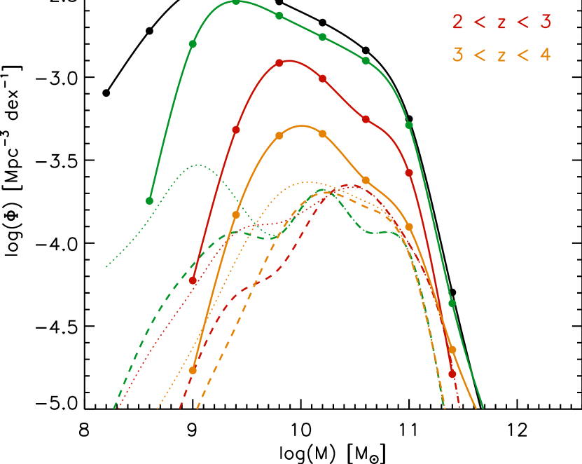
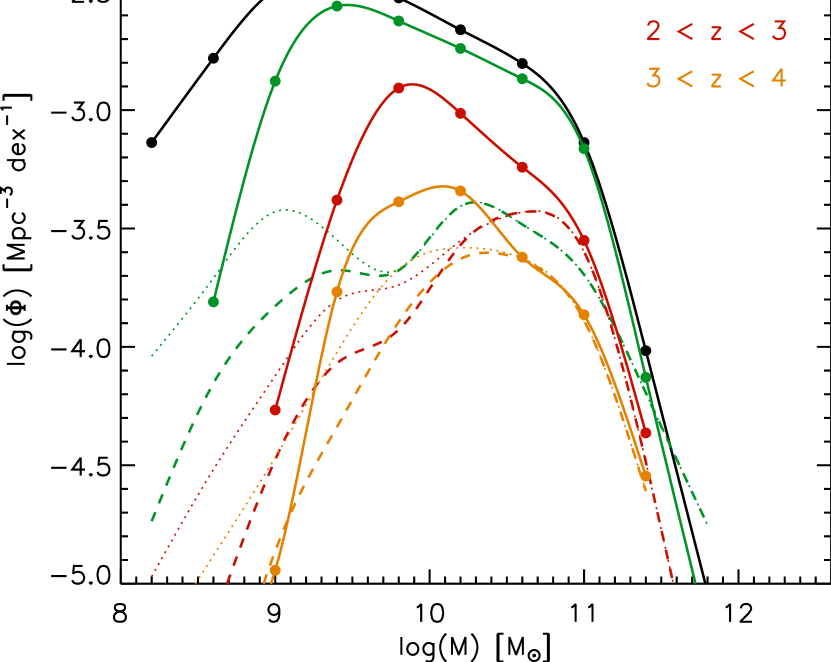
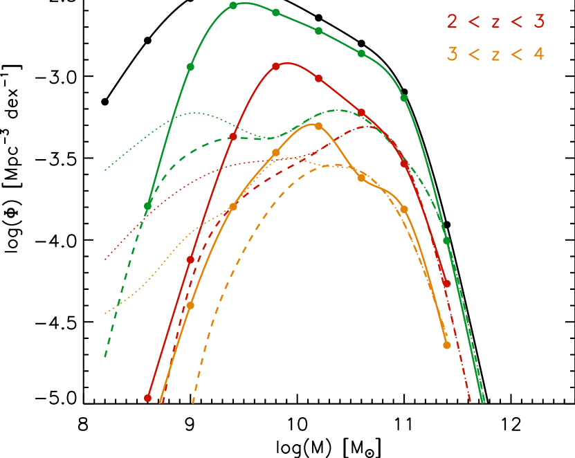
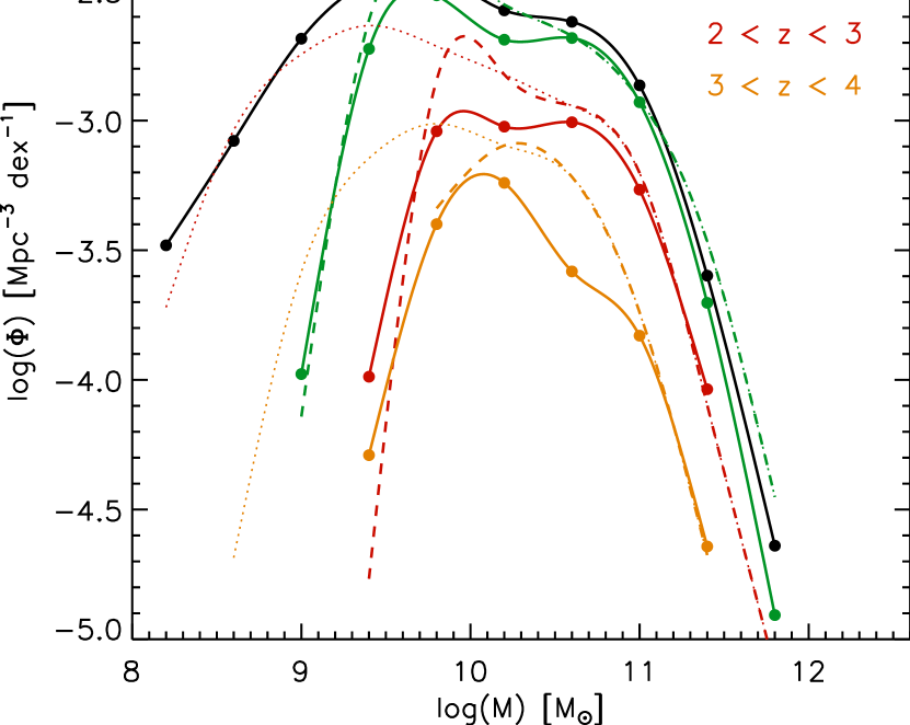
Figure 9.— Mass functions from $z=0$ to 4 as observed (solid curves), and as obtained by tracing lower-redshift galaxies back in time using the constraints on their SFHs from SED modeling (dotted curves). No incompleteness corrections are applied. Instead, dashed lines show the mass function of the traced-back populations after applying the $K=24.3$ magnitude limit. The following constraints were applied in modeling the SEDs with BC03 templates: (a) $\tau$ models with $\log(\tau_{min})=7.5$, (b) $\tau$ models with $\log(\tau_{min})=8.5$, (c) delayed $\tau$ models with $\log(\tau_{min})=8.5$, (d) delayed $\tau$ models with $\log(\tau_{min})=8.5$ and all galaxies being maximally old. Chi-square minimization prefers to fit steeply declining SFHs with young ages. Such solutions are physically unrealistic, as they violate the galaxy continuity equation as tested here. Instead, star formation over more prolonged timescales seems preferred.

6.2.2 Delayed $\tau$ Models

Recently, several authors have argued, both on observational (Renzini et al. 2009; Maraston et al. 2010; Papovich et al. 2011) and on theoretical (Finlator et al. 2007; Lee et al. 2010) grounds, that galaxies may undergo increasing, rather than decreasing, SFHs during parts of their life, specifically at early times ($z\gtrsim 3$). To allow for such phases of increasing SFR without imposing an artificial breakdown of our galaxy sample in sources fitted with strictly increasing versus sources fitted with strictly decreasing SFHs, we repeated our analysis using the following SFH:

$$SFR(t)=te^{-t/\tau}$$ (5)

These so-called delayed $\tau$ models allow for solutions with increasing SFRs (for ages $<\tau$) as well as solutions in which the SFR is decreasing after a prior phase during which it was increasing (for ages $>\tau$). At $t\ll\tau$, $SFR(M)\sim\sqrt{M}$ for delayed $\tau$ models as opposed to $SFR(M)\approx constant$ for simple $\tau$ models. This corresponds to evolutionary tracks with steeper initial slopes in the SFR-M diagram than default $\tau$ models, but still shallower than many literature values for the slope of the main sequence. The latter vary between this slope of a half and a slope of unity. Its precise value is still widely debated (Noeske et al. 2007; Cowie & Barger 2008; Pannella et al. 2009; Santini et al. 2009; Rodighiero et al. 2010), and may evolve with redshift (Dunne et al. 2009).

Figure 10a shows the $age/\tau$ ratio obtained by fitting delayed $\tau$ models to the SEDs of $0<z<4$ galaxies as function of SFR. Overall, only 20 % of the galaxies is best characterized by being observed during a phase in which the SFR is increasing ($age<\tau$). However, this fraction is a strong function of the level of star-forming activity (and therefore redshift). At SFRs above 10, 50, and 100 $M_{\sun}/yr$, galaxies that are best fit by rising SFRs account for 40, 60, and 70% of the overall population. At $z>2$, 37% of the galaxies in our $K<24.3$ sample are found to be in the rising part of their SFH (i.e., $age<\tau$). We note that the reduced chi-square ($\chi^{2}_{red}$) values of the fits with delayed $\tau$ models are indistinguishable from those obtained by fitting simple $\tau$ models. The SFR-weighted ages are in the median 0.1 dex older than those inferred from simple $\tau$ models, with a scatter of 0.15 dex, and a weak trend with age (the systematic offset being smaller for systems that formed the bulk of their stars more than a Gyr ago). Despite the modest increase in estimated ages, it is clear from Figure 8c and 9c that the underestimate of galaxy number densities at intermediate masses remains significant for this alternative SFH. In other words, in the absence of any stringent constraints on age, the delayed $\tau$ models are subject to the same outshining effect as were the simple $\tau$ models.

6.2.3 Maximally Early Onset of Star Formation

Finally, we repeat the population analysis once more, now making the assumption that all galaxies are maximally old (i.e., $age=t_{Hubble}(z_{obs})$). The SFR-weighted age $age_{w}$ may (and will) still be younger than the age of the universe at the epoch of observation, but we perform the SED modeling forcing the onset of star formation to take place at very high redshift. Given the discreteness in age of stellar population models, small variations in the adopted $z_{form}$ occur depending on the galaxy’s precise redshift, but it is typically around $z_{form}\sim 10$ and the precise value is irrelevant for this exercise. We again adopt delayed $\tau$ models, as they result in $\chi^{2}_{red}$ values that are better by a factor of $\sim 1.4$ than those obtained from fitting simple $\tau$ models with the same restriction on $z_{form}$. In practice, the least squares solution is now often one with $\tau>age$ (see the abundance of galaxies with $\log(age/\tau)<0$ in Figure 10b), such that the SFR-weighted age is minimized within the allowed range that goes from 0.5 (for $\tau\approx\infty$) to 1 (for $\tau\approx 0$) times the age of the universe at the observed epoch. These long e-folding times, obtained when maximizing the formation redshift, serve not to violate the constraints from the longer wavelengths on stellar mass, which tends to be the most robust parameter in SED modeling (e.g., Förster Schreiber et al. 2004; Shapley et al. 2005). Nevertheless, we do note that the median stellar mass of galaxies in our sample increases by 0.25 dex compared to SED modeling where no maximum formation redshift was imposed.

Although extreme, the assumption of maximally old galaxies is useful as a sanity check. If the backtraced galaxy samples are still underpopulated with respect to the observed samples, the origin of the discrepancy must most likely be attributed to other effects such as merging, cosmic variance, or more extreme SFHs in which an even larger fraction of the stellar mass was assembled at very early times. Figure 9d shows that this is not the case. At all redshifts, the backtraced mass functions match the observed mass functions surprisingly well, and are if anything slightly overproducing the number densities in some mass bins (an effect that is somewhat more pronounced if we had adopted simple $\tau$ models, that lead to even older SFR-weighted ages). We note that the SFR-M relation (Figure 8d) has tightened significantly by making the rigorous assumption on early formation epochs. This indicates that, aside from an intrinsic scatter owing to galaxy-to-galaxy differences in SFH, the scatter in the observed SFR-M relation also depends on model assumptions. Likewise, we find that conclusions on the differential evolution of the stellar mass function also depend on the assumed SFH. When making similar assumptions about the SFH as Marchesini et al. (2009), we confirm their finding of little evolution at the high-mass end, and much more at lower masses (see Figure 9b). When instead using delayed tau models in combination with tight constraints on the formation redshifts, the degree of such differential evolution reduces significantly (see Figure 9d).

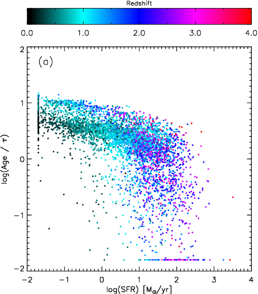
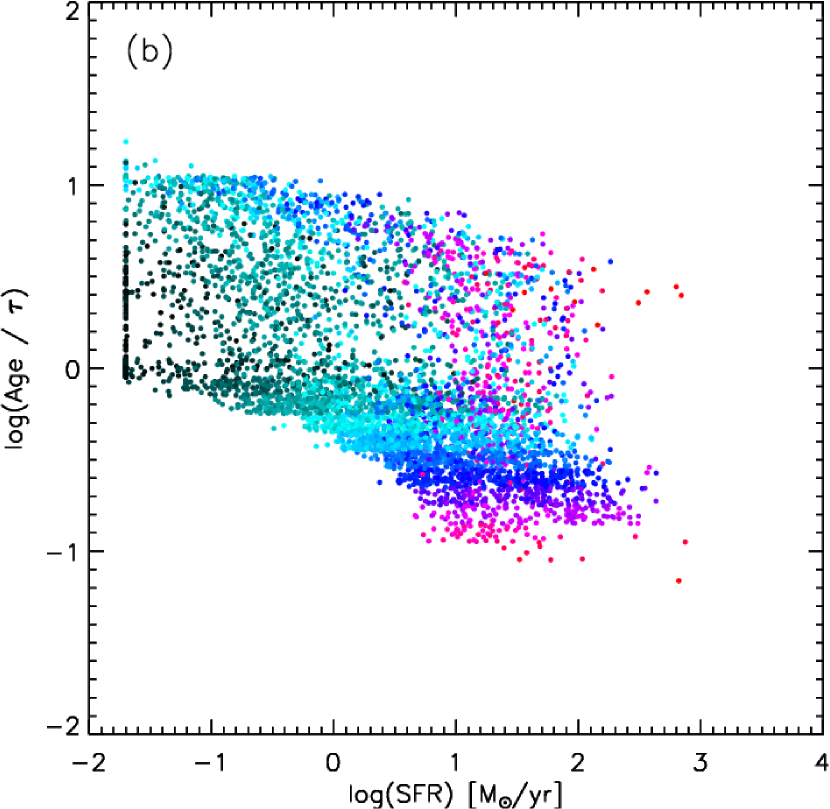
Figure 10.— Ratio of age (i.e., time since onset of star formation) over $\tau$ as function SFR for delayed $\tau$ models with (a) weak constraints on age (age $>50$ Myr), and (b) maximally old ages. When leaving age free, only a fraction of galaxies at the high SFR end is best modeled as following a rising SFH at the epoch of observation. When imposing very high formation redshifts ($z_{form}\sim 10$), larger values of $\tau$ ($>$ age) are preferred.

6.3. The Effect of Merging

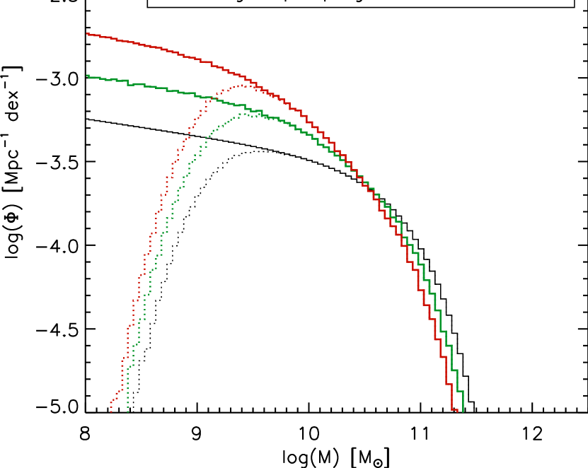
Figure 11.— Toy model exploring the impact of merging on tests of the galaxy continuity equation. Let the black curve be the high-redshift mass function as constructed by evolving a lower redshift observed galaxy population back in time, in the absence of merging. In a scenario where each galaxy underwent one merger between the low and high redshift bin, with mass ratio chosen randomly between 10:1 and 2:1, the green curve would be the resulting high-redshift mass function. Two merger events (red) or more per galaxy would steepen the mass function further.

So far, we assumed that each observed galaxy had only one progenitor that assembled its stellar mass by in situ star formation. In a hierarchical universe, where dark matter haloes merge to form increasingly larger structures, carrying with them the baryons that assembled at the centers of their potential wells, our simplified toy model must therefore fail to capture the detailed evolution of galaxy populations at some level. In order to properly account for galaxies merging (or in fact de-merging as we trace them back in time), an accurate knowledge of the merger rate as function of redshift, mass, and mass ratio would be required. Moreover, the probability that a galaxy observed at redshift $z_{obs}$ underwent a merger since redshift $z_{obs}+\Delta z$ (and hence has to be split in two as we trace it back to that epoch) may not only depend on its mass. For example, if merging leads to quenching (e.g., Di Matteo et al. 2005), a quiescent galaxy may be more likely to have undergone a merger in its past than a star-forming galaxy of similar mass. Furthermore, it is well motivated that mergers between gas-rich systems trigger starbursts in their centers, which inhibits evolving galaxies back along smooth tracks in the SFR-M diagram. In fact, the scatter in the SFR-M relation of star-forming galaxies may well be produced by such burstiness, triggered by (minor) mergers or other processes. Clearly, implementing all of these processes in our consistency check is beyond the scope of this paper. We therefore choose to illustrate the effect of merging activity on our analysis by two models of increasing complexity.

6.3.1 A Simple Toy Model for Merging

The first is an idealized toy model, presented in Figure 11. Here, the black curve represents a hypothetical mass function at $z_{obs}+\Delta z$ as traced back from galaxies observed at $z_{obs}$. The dotted line accounts for the magnitude limit of our catalog. If every galaxy observed at $z_{obs}$ underwent one merger in the interval $\Delta z$ (for simplicity we assume one that did not affect the SFH), the actual number of progenitors will be twice as large as anticipated in the absence of merging. Since the mass distribution of progenitors will be shifted to lower values, the number of galaxies entering our magnitude-limited catalog will be larger by a somewhat smaller factor. Under the assumption of a merger rate that is a constant function of the mass ratio over the range 10:1 to 2:1, the resulting mass function is plotted in green. If all of these merger progenitors themselves descended from mergers taking place since $z_{obs}+\Delta z$, the red curve would be the backtraced population (consisting of four times as many galaxies as observed at $z_{obs}$, ignoring incompleteness issues). The net effect is a steepening of the mass function, the magnitude of which depends on the amplitude of the merger rate.

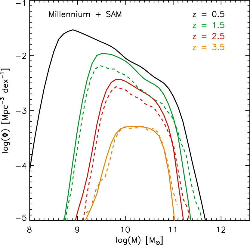
Figure 12.— Stellar mass functions down to an observed $K$-band magnitude of 24.3 derived from the De Lucia & Blaizot (2007) SAM which is based on the Millennium Simulation (solid lines). Dashed lines indicate the mass functions at $z=1.5$, 2.5 and 3.5, constructed after summing those galaxies that have a common descendant at $z=0.5$, 1.5 and 2.5 respectively. Accounting for merging as we track galaxies back in time (solid lines) steepens the mass function with respect to an approach that ignores merging (dashed lines).

6.3.2 Merging in Semi-Analytic Models

While conceptually demonstrating the impact of merging, our toy model does not contain information on the frequency of galaxy collisions, and therefore its conclusions remain qualitative at best. In order to obtain a more quantitative estimate, we turn to a second, more physically motivated model in Figure 12. Here, the solid lines mark the galaxy stellar mass functions at a range of redshifts as extracted from the Munich semi-analytic model (SAM) of galaxy formation by De Lucia & Blaizot (2007). The SAM is rooted in the pure dark matter Millennium Simulation (Springel et al. 2005), and hence incorporates the hierarchical mass build-up characteristic for a $\Lambda$-CDM cosmology. It furthermore contains a set of prescriptions to model the baryonic physics within this framework, and outputs among other parameters the observed-frame photometry, which we use to apply the $K$-band magnitude limit of the observations. Here, we will not focus on differences between the model and observed mass functions (most notably a relatively late build-up of the high-mass end and early build-up of the low-mass end in the SAM), these are discussed at length by Marchesini et al. (2009). Instead, we use the SAM with its physically motivated merger rates as a self-consistent testbed to constrain the impact of merging activity.

Since the merger tree of each galaxy is stored, it is trivial to perform our analysis from Section 6.1 on the SAM, i.e., to evolve galaxies back in time according to their SFH ignoring merging. For example, to obtain the inferred population at $z=2.5$ by winding back the clock from $z=1.5$, we simply group all $z=2.5$ galaxies that have a common descendant at $z=1.5$, sum their masses, and construct the mass function from the resulting sample (red dashed line in Figure 12). In the SAM, by construction, any difference between the backtraced and actual mass function at a given redshift is due to merging. As expected from our simplistic toy model (Figure 11), the net effect of including merging is a steepening of the mass function: while the high-mass end is reduced, the number density at intermediate masses increases by 0.25 dex, 0.15 dex and 0 dex at $z=1.5$, 2.5 and 3.5 respectively.

We conclude that accounting for mergers will reduce the discrepancy in number densities seen in Section 6.2 at low to intermediate masses, but typical merger rates from dark matter + semi-analytic models seem insufficient to fully resolve the underdensities we found. Invoking more active merger histories would break down the good agreement at the high-mass end ($M\gtrsim 10^{11}\ M_{\sun}$) by suppressing the abundance of those galaxies. Given these concerns, we now turn to what is likely a major contributor to the offsets between the observed and backtraced mass functions in Figure 9a-c: biases in characterizing the galaxy-averaged stellar age.

6.4. Constraining Galaxy Ages

In Section 6.2, we found that the backtraced and observed mass functions over a wide range of redshifts matched better when forcing maximally old ages in the SED modeling. Although merging and stochastic bursts will undoubtly affect the evolutionary tracks of galaxies in the SFR-M diagram, it seems unlikely that they can account for the discrepancies observed when leaving formation redshifts as a free parameter in the SED modeling. We therefore turn to the measurement of galaxy ages, and discuss two avenues for improvement.

6.4.1 Extending the Wavelength Range

First, it is illustrative to contrast the best-fit stellar population models with and without the constraint of a maximally early onset of star formation. The top two panels in Figure 13 show the SEDs of two quiescent galaxies at $z\sim 1.5$, while the bottom three panels represent cases at the same redshift of galaxies populating the main sequence of star formation. Irrespective of galaxy type, we note that both the free age and the maximally old best-fit model reproduces the broad-band SEDs remarkably well. By and large, the two templates are indistinguishable for broad-band tracers, except at rest-frame wavelengths shortward of 0.2 $\mu$m, and to a lesser extent at the longest wavelengths probed ($\lambda_{rest}\gtrsim 2.5\mu$m). Present-day stellar population synthesis codes are facing the largest differences in the latter regime (Maraston 2005). We therefore conclude that more stringent constraints on the $\lambda_{rest}<0.2\mu$m SED, from deep FUV, NUV, and $U$-band observations, would help most to better constrain galaxy stellar ages without the need to impose ad hoc constraints on formation redshifts. Rettura et al. (2010), among others, recognize this, and succesfully exploit rest-frame UV data of $z\sim 1.2$ ellipticals in clusters and field environments to constrain both their onset and timescale of star formation.

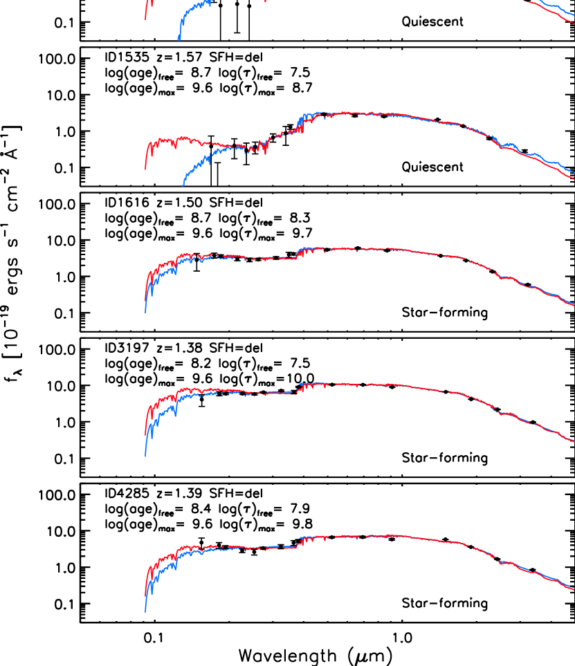
Figure 13.— Rest-frame broad-band SEDs of $z\sim 1.5$ galaxies, with best-fit BC03 template leaving age free (blue), or forcing a maximally old onset of star formation (red). The top two panels present quiescent galaxies, whereas the bottom three panels present SEDs of galaxies on the main sequence of star formation. Stronger observational constraints on the rest-frame 0.1 - 0.2 $\mu$m regime are desired to improve the estimate of stellar ages.

6.4.2 Resolved SED Modeling

A second avenue for improvement concerns not so much the wavelength range, but rather the scales probed with multi-wavelength photometry. The outshining effect that limits our ability to constrain galaxy ages results from an older, underlying stellar population whose existence is not captured by the best-fit SFH because the SED is dominated by the younger and less obscured part of the stellar population. If such multiple components of the galaxy’s SFH are spatially disjoint, as might be expected, we may bypass or at least reduce the outshining effect by means of resolved SED modeling. The advent of the WFC3 camera onboard HST, in concert with the long-time workhorse ACS, opens a window on such analyses. Wuyts et al. (in prep) present in detail the implications of resolved stellar populations at high redshift, but for our present purpose we focus solely on the estimate of SFR-weighted ages (i.e., the age of the bulk of the stars). Here, we use the WFC3 $Y$, $J$, and $H$ data of the Early Release Science (ERS) program as testbed, in combination with ACS $B$, $V$, $i$, $z$ data in GOODS-South matched to the same resolution (0.16”, sampled by a 0.06”/pix drizzled pixelscale). For a sample of 282 galaxies with $K<24.3$ and $1.5<z<2.5$, we perform a default SED modeling analysis on the summed BVizYJH photometry of all galaxy pixels with $S/N_{H}>3$. We ignore any aperture corrections, which may well be important for estimates of, e.g., total stellar mass if a substantial fraction of the galaxy mass resides in the outskirts where pixels have $S/N_{H}<3$. However, it is irrelevant for our present discussion on galaxy age and how its estimate depends on an integrated versus resolved approach, because in both cases we work with the same set of pixels (namely those with $S/N_{H}>3$). Next, we run the SED modeling procedure on a pixel-by-pixel basis, yielding a best-fit mass, age, $\tau$, and $A_{V}$ for each object pixel individually. Our approach is similar in spirit to the recent study by Zibetti, Charlot & Rix 2009 who spatially resolve the stellar populations in nearby galaxies (obviously to scales much smaller than probed in our high-redshift sample). We confirm that the sum of all best-fit templates from the pixel-by-pixel analysis provides an excellent match to the integrated galaxy SED. In Figure 14, we compare the SFR-weighted age obtained from pixel-by-pixel SED modeling to that preferred by fitting one $\tau$ model to the integrated galaxy photometry. Here, the SFR-weighted age inferred from resolved SED modeling is computed following equation 4, but the effective SFH over which one integrates is now not a simple $\tau$ model, but the superposition of $\tau$ models, each with their own normalization, $\tau$ and age, for each of the object pixels. We observe a clear trend of increased inferred stellar ages, ranging from 0 to 2 orders of magnitude, when adopting a resolved SED modeling approach. The offsets are small for galaxies where integrated SED modeling indicates old stellar populations and low SFRs, specific SFRs, and visual extinctions. For systems where younger ages, and higher SFRs, SFR/M, and $A_{V}$ are inferred from integrated SED modeling, the age correction factors exhibit a large scatter. Formally, the offsets correlate most strongly with galaxy age. We derive a mean correction

$$\log age_{w,resolved}=6.86-1.75\log age_{w,integrated}$$ (6)

with a scatter increasing from 0.1 dex for the systems with the oldest $age_{w,integrated}$ to 0.4 dex for those with the youngest $age_{w,integrated}$.

Figure 14.— Comparison of the SFR-weighted age of galaxies with $K<24.3$ at $1.5<z<2.5$, as determined by fitting simple $\tau$ models to the ACS/WFC3 $BVizYJH$ photometry of each object pixel individually, versus fitting a simple $\tau$ model to the integrated SED. Spatially resolved SED modeling results in higher age estimates since variations in SFH on galaxy-wide scales can be accounted for, hence reducing the outshining effect by young stars.

This behavior may partially be driven by the condition that the time since the onset of star formation must be less than the age of the universe at the epoch of observation (galaxies with old $age_{w,integrated}$ already lie close to this upper bound). We do find only a very weak correlation with angular size (i.e., the number of independent resolution elements in which the galaxies are resolved), a property that itself correlates, at a given mass, with star formation activity (Franx et al. 2008; Toft et al. 2009).

In order to rule out any systematic biases by fitting to the low S/N SEDs of individual pixels, we applied the same integrated and resolved SED modeling procedure to a set of 500 mock galaxies with a uniform stellar population and representative stellar masses, sizes, and $H$-band pixel flux distributions. Our toy galaxies vary in e-folding time between 30 Myr and 3 Gyr, in the time since the onset of star formation between 100 Myr and the age of the universe, and were attenuated by a uniform visual extinction of $A_{V}=1$. We computed their broad-band SEDs as observed at $z=2$, and disturbed the pixel fluxes appropriately according to the pixel-to-pixel rms of the real data. We confirm that both the integrated and resolved SED modeling methods correctly recover the input SFR-weighted ages, to within a few percent. The central 68th percentile interval of the $\Delta\log age_{w}$ distribution broadens by 35% for resolved compared to integrated SED modeling, but no systematic bias is introduced by the method. Based on this sanity check, we can state with confidence that the systematic offsets observed for the ERS2 galaxies are due to real spatial variations in their stellar populations.

Given the limited resolution, we can only account for differences in SFH across the largest galaxy-wide scales. The outshining may well remain present on scales below the resolution of the WFC3 imaging (0.16” FWHM, corresponding to 1.3 kpc at $z=2$, sampled by drizzled pixels of 0.06”). We note that the effective visual attenuation $A_{V,resolved}$, computed as

$$A_{V,resolved}=2.5\log\left(\sum_{i=1}^{Npix}L_{V,intrinsic,i}\right)$$

$$-2.5\log\left(\sum_{i=1}^{Npix}L_{V,attenuated,i}\right),$$ (7)

also increases when performing resolved SED modeling, by $0.2^{+0.6}_{-0.2}$ mag. This technique may therefore help to alleviate both the outshining effect and the saturation of reddening by patchy dust obscuration (see Section 4.1). Obviously, its use is limited to special data sets rich in multi-wavelength high-resolution imaging. Finally, despite the strong observed trends, we caution that SED modeling on an individual pixel basis is still subject to the same age-dust degeneracy that is well-known from integrated SED modeling, particularly when based on the relatively narrow observed $B$-to-$H$ wavelength baseline.

7. Summary

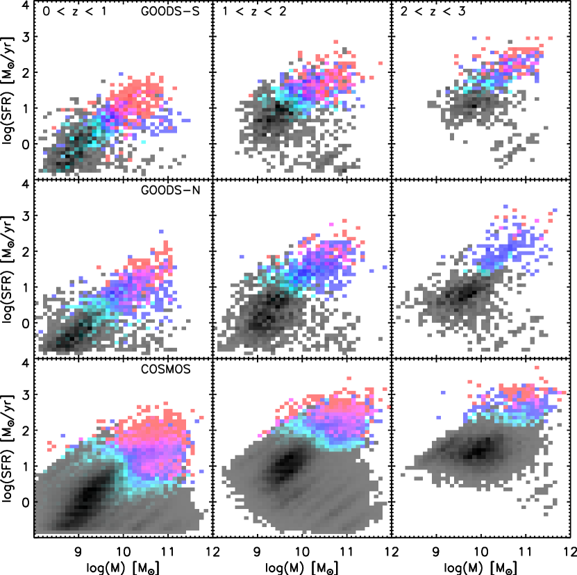
Figure 15.— SFR versus mass diagram in the GOODS-South, GOODS-North, and COSMOS field. The color-coding illustrates the SFR indicator used, from SED modeling for all galaxies in a SFR-mass bin (black) to $SFR_{UV+PACS}$ for all galaxies in a SFR-mass bin (red). Blue regions contain predominantly galaxies with $SFR_{UV+24\mu m}$ as primary SFR indicator. A combination of SFR indicators, as cross-calibrated in this paper, is necessary to fully probe the main sequence of star formation, particularly in wider fields with shallower PACS and MIPS depths.

We compared SFR indicators out to redshift $z=3$ relying on PACS far-infrared, MIPS 24 $\mu$m, and UV emission, $U$-to-8 $\mu$m SED modeling, as well as H$\alpha$ spectroscopy. Figure 15 illustrates that, in order to study the entire galaxy population (above a certain mass) out to high redshift, a combination of self-consistent SFR indicators is required. This applies even more so to studies that exploit larger areas that often received only shallower PACS and/or MIPS imaging. This study aims at providing such a series of cross-calibrated recipes. In Wuyts et al. (2011b), we exploit this continuity across SFR indicators in concert with high-resolution HST imaging to address the relation between the level and mode of star formation, and its mass dependence.

Using the deeper PEP data in GOODS-South, we confirm previous reports by Nordon et al. (2010) and Elbaz et al. (2010) that luminosity-dependent conversions from observed 24 $\mu$m to $L_{IR}$ based on the CE01 and DH02 template libraries lead to overestimated $L_{IR}$ (and hence SFRs) at the highest SFRs ($SFR>100\ M_{\sun}/yr$) and redshifts ($z>1.5$). This trend is also consistent with early findings by Papovich et al. (2007) on the basis of stacking of MIPS 70 $\mu$m and 160 $\mu$m data. Using the luminosity-independent conversion by W08, which is based on a template with enhanced PAH emission relative to local ULIRGs, gives $L_{IR}$ based on 24 $\mu$m that are in the median consistent with PACS photometry, although with a 0.25 dex scatter.

SED modeling recipes can be tuned to reproduce $SFR_{UV+IR}$ for systems with low to intermediate SFRs (e.g., by adjusting the minimum allowed e-folding time for exponentially declining SFHs). The relatively long (at least several 100 Myr) e-folding times required for SED modeling with BC03 to match $SFR_{UV+IR}$ implies that most star formation happened in a relatively stable mode, varying slowly on timescales that correspond to of order $\sim 50$ dynamical times.

Galaxies at the high SFR end ($SFR\gtrsim 100\ M_{\sun}/yr$) tend to be dusty, and are increasingly common toward high redshifts. Simple dust correction methods assuming a uniform foreground screen fail to recover their total amount of star formation. Due to the patchiness of the dust distribution in these objects, reddening saturates as a tracer of extinction. This bias applies to SED modeling as well as methods based on single colors, that are designed for a specific (high) redshift range (Daddi et al. 2007a). At the low SFR end, we find a hint of steeper, more SMC-like extinction curves than the Calzetti et al. (2000) law. Such a trend could occur if a lower gas density in those systems lead to a size distribution of the dust grains mixed with the gas that is biased to small grains.

SFRs based on H$\alpha$ luminosities of star-forming galaxies at $z\sim 2$ show a good correspondence to $SFR_{UV+IR}$ and $SFR_{SED}$, provided we account for extra attenuation towards HII regions compared to the stellar continuum (see also Förster Schreiber et al. 2009). The locally calibrated scaling $A_{V,neb}=A_{V,SED}/0.44$ holds out to $z\approx 2.6$. Since the SINS H$\alpha$ measurements were obtained in integral field mode, our conclusion is not subject to uncertainties in slit correction factors.

Next, we fixed the SFR in SED modeling to $SFR_{UV+IR}$, avoiding biases inherent to dust correction methods and reducing the degrees of freedom by one. The SFHs inferred from SED modeling are tested for consistency with a no-merger galaxy continuity equation. Briefly, we compared the observed SFR-M relation and mass function at a range of redshifts to backtraced analogs based on evolving the observed galaxy population at lower redshifts back in time. We find the locus of the main sequence of star formation to be well reproduced by the backtraced model. However, number densities of intermediate- to low-mass galaxies are underestimated. This discrepancy is observed both for simple $\tau$ models and delayed $\tau$ models. Accounting for mergers is unlikely to resolve the discrepancy without removing the agreement at the high-mass end. A better agreement is only obtained when forcing early formation redshifts.

Independent evidence from resolved SED modeling also implies that stellar population modeling of integrated photometry leads to age underestimates. Resolving regions that underwent different SFHs helps to reduce the effect of outshining of old stellar populations by the youngest generation of stars. Alternatively, higher $S/N$ data extending to shorter rest-wavelengths $\lambda_{rest}<0.2\mu$m would provide more leverage on the stellar age.

The authors acknowledge Mariska Kriek for use of the FAST stellar population fitting code. S. W. wishes to thank Roderik Overzier for stimulating discussions. The Millennium Simulation databases used in this paper and the web application providing online access to them were constructed as part of the activities of the German Astrophysical Virtual Observatory.

APPENDIX

One concern in exploiting 24 $\mu$m emission as SFR indicator for high-redshift galaxies is a possible contribution from hot dust heated by an Active Galactic Nucleus (AGN) rather than young stars. In order to investigate the potential bias induced by AGN in our sample, we mark all galaxies associated with an X-ray source brighter than $L_{X}>10^{42}\ erg\ s^{-1}$ in the rest-frame 2 - 10 keV band with a black open circle in Figure 2. Here, the X-ray luminosities were calculated based on the galaxy’s redshift, and the full band flux and spectral index from the Luo et al. (2008) 2 Ms Chandra catalog, which we cross-correlated with the FIREWORKS catalog using a search radius of 1”. We note that, owing to the deeper PEP observations in GOODS-South, the fraction of X-ray AGN with a significant ($>3\sigma$) PACS detection is larger ($\sim 35$%) than the 20% found in GOODS-North by Shao et al. (2010). However, among the total sample of PACS-detected sources, X-ray AGN form a minority ($<10$%).

While the X-ray selected AGN typically have residuals $\nu f_{\nu}/\nu f_{\nu,template}<1$ in Figure 2b (for a given IR luminosity, they are brighter at 24 $\mu$m than the overall PACS-detected galaxy population by a median factor 1.4), excluding them changes the median binned values (filled black symbols in Figure 2b) by less than 8% only. We conclude that, whereas contribution by AGN can significantly affect the mid- to far-IR SEDs of individual galaxies, their relative number is sufficiently small that our above result for the ensemble of PACS-detected galaxies out to $z=3$ is robust against such a bias. We do however caution that this assessment of AGN contribution relies on the assumption that all AGN responsible for hot dust emission have $L_{X}>10^{42}\ erg\ s^{-1}$. If a substantial population of Compton thick AGN, undetected at X-ray wavelengths, exists (Daddi et al. 2007b), other indicators of AGN activity such as a power-law shape of the SED in the rest-frame 1 - 10 $\mu$m regime (see, e.g., Park et al. 2010) have to be explored to properly infer SFRs from dust re-emission. Exploiting the combination of PACS and Chandra data in GOODS-North, Shao et al. (2010) find that the far-infrared luminosity of high-redshift AGN shows little dependence on the X-ray obscuring column and the AGN luminosity. Finally, we note that ultra-deep IRS spectroscopy of $z\sim 1$ LIRGs and $z\sim 2$ ULIRGs (Fadda et al. 2010) found that both categories are starburst dominated. Based on the strong PAH emission in their IRS spectra, Fadda et al. (2010) conclude that the compton thick AGN contribution to the bolometric luminosity of $z\sim 2$ ULIRGs is substantially lower than previously inferred by Daddi et al. (2007b). Nordon et al. (2011) also argue for an enhanced presence of PAHs in star-forming $z\sim 2$ galaxies, rather than systematic boosting of 24 $\mu$m fluxes by AGN.

References

- (1) Bell, E. F., McIntosh, D. H., Katz, N.,& Weinberg, M. D. 2003, ApJS, 133149, 289
- (2) Bell, E. F., et al. 2005, ApJ, 625, 23
- (3) Berta, S., et al. 2010, A&A, 518, 30
- (4) Borch, A., et al. 2006, A&A, 453, 869
- (5) Bouchet, P., Lequeux, J., Maurice, E., Prévot, L.,& Prévot-Burnichon, M. L. 1985, A&A, 149, 330
- (6) Bouwens, R. J., Illingworth, G. D., Franx, M.,& Ford, H. 2007, ApJ, 670, 928
- (7) Bouwens, R. J., et al. 2010, in prep (arXiv1006.4360)
- (8) Brammer, G. B., van Dokkum, P. G.,& Coppi, P. 2008, ApJ, 686, 1503
- (9) Bruzual, G,& Charlot, S. 2003, MNRAS, 344, 1000
- (10) Bundy, K., et al. 2006, ApJ, 651, 120
- (11) Calzetti, D., Kinney, A. L.,& Storchi-Bergmann, T. 1994, ApJ, 429, 582
- (12) Calzetti, D., Armus, L., Bohlin, R. C., Kinney, A. L., Koornneef, J.& Storchi-Bergmann, T. 2000, ApJ, 533, 682
- (13) Cassisi, S., Castellani, M.,& Castellani, V. 1997, A&A, 317, 108
- (14) Chabrier, G. 2003, PASP, 115, 763
- (15) Chary, R.,& Elbaz, D. 2001, ApJ, 556, 562
- (16) Cid-Fernandes, R., Mateus, A., Sodré, L. Jr., Stasinska, G.,& Gomes, J. M. 2005, MNRAS, 358, 363
- (17) Cole, S., et al. 2001, MNRAS, 326, 255
- (18) Cowie, L. L.,& Barger, A. J. 2008, ApJ, 686, 72
- (19) Daddi, E., Cimatti, A., Renzini, A., Fontana, A., Mignoli, M., Pozzetti, L., Tozzi, P.,& Zamorani, G. 2004, ApJ, 617, 746
- (20) Daddi, E., et al. 2007a, ApJ, 670 156
- (21) Daddi, E., et al. 2007b, ApJ, 670, 173
- (22) Dale, D. A.,& Helou, G. 2002, ApJ, 576, 159
- (23) Damen, M., Förster Schreiber, N. M., Franx, M., Labbé, I., Toft, S., van Dokkum, P. G.,& Wuyts, S. 2009, ApJ, 705, 617
- (24) Davé, R. 2008, MNRAS, 385, 147
- (25) De Lucia, G.,& Blaizot, J. 2007, MNRAS, 375, 2
- (26) Dickinson, M., Papovich, C., Ferguson, H. C.,& Budavári, T. 2003, ApJ, 587, 25
- (27) Di Matteo, T., Springel, V.,& Hernquist, L. 2005, Nature, 433, 604
- (28) Drory, N., Bender, R., Feulner, G., Hopp, U., Maraston, C., Snigula, J.,& Hill, G. J. 2004, ApJ, 608, 742
- (29) Drory, N., Salvato, M., Gabasch, A., Bender, R., Hopp, U., Feulner, G.,& Pannella, M. 2005, ApJ, 619, L111
- (30) Dunne, L., Ivison, R. J., Maddox, S., et al. 2009, MNRAS, 394, 3
- (31) Elbaz, D., et al. 2007, A&A, 468, 33
- (32) Elbaz, D., et al. 2010, A&A, 518, 29
- (33) Elmegreen, B. 1997, Rev. Mex. Astron. Astrofis., 6, 165
- (34) Erb, D. K., Steidel, C. C., Shapley, A. E., Pettini, M., Reddy, N. A.,& Adelberger, K. L. 2006, ApJ, 647, 128
- (35) Fadda, D., et al. 2010, ApJ, 719, 425
- (36) Elsner, F., Feulner, G.,& Hopp, U. 2008, A&A, 477, 503
- (37) Fagotto, F., Bressan, A., Bertelli, G.,& Chiosi, C. 1994, A&AS, 104, 365
- (38) Finlator, K., Davé, R.,& Oppenheimer, B. D. 2007, MNRAS, 376, 1861
- (39) Fontana, A., et al. 2003, A&A, 594, L9
- (40) Fontana, A., et al. 2004, A&A, 424, 23
- (41) Fontana, A., et al. 2006, A&A, 459, 745
- (42) Fontana, A., et al. 2009, A&A, 501, 15
- (43) Förster Schreiber, N. M., Genzel, R., Lutz, D., Kunze, D.,& Sternberg, A. 2001, ApJ, 552, 544
- (44) Förster Schreiber, N. M., et al. 2004, ApJ, 616, 40
- (45) Förster Schreiber, N. M., et al. 2006, ApJ, 645, 1062
- (46) Förster Schreiber, N. M., et al. 2009, ApJ, 706, 1364
- (47) Franx, M., van Dokkum, P. G., Förster Schreiber, N. M., Wuyts, S., Labbé, I.,& Toft, S. 2008, ApJ, 688, 770
- (48) Genzel, R., et al. 2006, Nature, 442, 786
- (49) Genzel, R., et al. 2008, ApJ, 687, 59
- (50) Genzel, R., et al. 2010, MNRAS, 407, 2091
- (51) Giavalisco, M., et al. 2004, ApJ, 600, L103
- (52) Goldader, J. D., Meurer, G., Heckman, T. M., Seibert, M., Sanders, D. B., Calzetti, D.,& Steidel, C. C. 2002, ApJ, 568, 651
- (53) Hopkins, A. M.,& Beacom, J. F. 2006, ApJ, 651, 142
- (54) Kajisawa, M., Ichikawa, T., Yamada, T., Uchimoto, Y. K., Yoshikawa, T., Akiyama, M.,& Onodera, M. 2010, ApJ, 723, 129
- (55) Kennicutt, R. C. 1998, ARA&A, 36, 189
- (56) Kriek, M., et al. 2006, ApJ, 649, 71
- (57) Kriek, M., van Dokkum, P. G., Labbé, I., Franx, M., Illingworth, G. D., Marchesini, D.,& Quadri, R. F. 2009, ApJ, 700, 221
- (58) Labbé, I., et al. 2005, ApJ, 624, 81
- (59) Lee, S.-K., Ferguson, H. C., Somerville, R. S., Wiklind, T.,& Giavalisco, M. 2010, ApJ, 725, 1644
- (60) Lilly, S. J., Le Fèvre, O., Hammer, F.,& Crampton, D. 1996, ApJ, 460, L1
- (61) Luo, B., et al. 2008, ApJS, 179, 19
- (62) Madau, P., Ferguson, H. C., Dickinson, M. E., Giavalisco, M., Steidel, C. C.,& Fruchter, A. 1996, MNRAS, 283, 1388
- (63) Magdis, G. E., et al. 2010, MNRAS, 409, 22
- (64) Magnelli, B., Elbaz, D., Chary, R. R., Dickinson, M., Le Borgne, D., Frayer, D. T.,& Willmer, C. N. A. 2009, A&A, 496, 57
- (65) Maiolino, R.,& Natta, A. 2002, Ap&SS, 281, 233
- (66) Maraston, C. 2005, MNRAS, 362, 799
- (67) Maraston, C., Daddi, E., Renzini, A., Cimatti, A., Dickinson, M., Papovich, C., Pasquali, A.,& Pirzkal, N. 2006, ApJ, 652, 85
- (68) Maraston, C., Pforr, J., Renzini, A., Daddi, E., Dickinson, M., Cimatti, A.,& Tonini, C. 2010, MNRAS, 407, 830
- (69) Marchesini, D., van Dokkum, P. G., Förster Schreiber, N. M., Franx, M., Labbé, I.,& Wuyts, S. 2009, ApJ, 701, 1765
- (70) Meurer, G. R., Heckman, T. M.,& Calzetti, D. 1999, ApJ, 521, 64
- (71) Muzzin, A., van Dokkum, P. G., Kriek, M., Labbé, I., Cury, I., Marchesini, D.,& Franx, M. 2010, ApJ, 725, 742
- (72) Noeske, K. G., et al. 2007, ApJ, 660, 43
- (73) Nordon, R., et al. 2010, A&A, 518, 24
- (74) Onodera, M., Arimoto, N., Daddi, E., Renzini, A., Kong, X., Cimatti, A., Broadhurst, T.,& Alexander, D. M. 2010, ApJ, 715, 385
- (75) Pannella, M. Carilli, C. L., Daddi, E., et al. 2009, ApJ, 698, L116
- (76) Papovich, C., et al. 2007, ApJ, 668, 45
- (77) Papovich, C., Finkelstein, S. L., Ferguson, H. C., Lotz, J. M,& Giavalisco, M. 2011, MNRAS, 412, 1123
- (78) Park, S. Q., et al. 2010, ApJ, 717, 1181
- (79) Peng, C. Y., Ho, L. C., Impey, C. D.,& Rix, H.-W. 2010, AJ, 139, 2097
- (80) Pérez-González, P. G., et al. 2008, ApJ, 675, 261
- (81) Poggianti, B. M., Bressan, A.,& Franceschini, A. 2001, ApJ, 550, 195
- (82) Poglitsch, A., et al. 2010, A&A, 518, 2
- (83) Pozzetti, L., et al. 2007, A&A, 474, 443
- (84) Prévot, M. L., Lequeux, J., Prévot, L., Maurice, E.,& Rocca-Volmerange, B. 1984, A&A, 132, 389
- (85) Reddy, N. A.,& Steidel, C. C. 2009, ApJ, 692, 778
- (86) Reddy, N. A., Erb, D. K., Pettini, M., Steidel, C. C., Shapley, A. E. 2010, ApJ, 712, 1070
- (87) Renzini, A. 2009, MNRAS, 398, 58
- (88) Rettura, A., et al. 2010, ApJ, 709, 512
- (89) Rodighiero, G., et al. 2010, A&A, 518, 25
- (90) Santini, P., et al. 2009, A&A, 504, 751
- (91) Schiminovich, D., et al. 2005, ApJ, 619, L47
- (92) Schmidt, M. 1959, ApJ, 129, 243
- (93) Shao, L., et al. 2010, A&A, 518, 26
- (94) Shapley, A. E., Steidel, C. C., Erb, D. K., Reddy, N. A., Adelberger, K. L., Pettini, M., Barmby, P.,& Huang, J. 2005, ApJ, 626, 698
- (95) Silk, J. 1997, ApJ, 481, 703
- (96) Somerville, R. S., Lee, K., Ferguson, H. C., Gardner, J. P., Moustakas, L. A.,& Giavalisco, M. 2004, ApJ, 600, 171
- (97) Springel, V., et al. 2005, Nature, 435, 629
- (98) Steidel, C. C., Adelberger, K. L., Giavalisco, M., Dickinson, M.,& Pettini, M. 1999, ApJ, 519, 1
- (99) Symeonidis, M., Page, M. J.,& Seymour, N. 2011, MNRAS, 411, 983
- (100) Toft, S., Franx, M., van Dokkum, P., Förster Schreiber, N. M., Labbé, I., Wuyts, S.,& Marchesini, D. 2009, ApJ, 705, 255
- (101) Vergani, D., et al. 2008, A&A, 487, 89
- (102) Wolf, C., Meisenheimer, K., Rix, H.-W., Borch, A., Dye, S.,& Kleinheinrich, M. 2003, A&A, 401, 73
- (103) Wuyts, S., et al. 2007, ApJ, 655, 51
- (104) Wuyts, S., Labbé, I., Förster Schreiber, N. M., Franx, M., Rudnick, G., Brammer, G. B.,& van Dokkum, P. G. 2008, ApJ, 682, 985
- (105) Wuyts, S., Franx, M., Cox, T. J., Hernquist, L., Hopkins, P. F., Robertson, B. E.,& van Dokkum, P. G. 2009a, ApJ, 696, 348
- (106) Wuyts, S., et al. 2009b, ApJ, 700, 799
- (107) Yoshikawa, T., et al. 2010, ApJ, 718, 112
- (108)