Anomalous Aharonov–Bohm gap oscillations in carbon nanotubes

Abstract

The gap oscillations caused by a magnetic flux penetrating a carbon nanotube represent one of the most spectacular observation of the Aharonov–Bohm effect at the nano–scale. Our understanding of this effect is, however, based on the assumption that the electrons are strictly confined on the tube surface, on trajectories that are not modified by curvature effects. Using an ab initio approach based on Density Functional Theory we show that this assumption fails at the nano–scale inducing important corrections to the physics of the Aharonov–Bohm effect. Curvature effects and electronic density spilled out of the nanotube surface are shown to break the periodicity of the gap oscillations. We predict the key phenomenological features of this anomalous Aharonov–Bohm effect in semi–conductive and metallic tubes and the existence of a large metallic phase in the low flux regime of Multi-walled nanotubes, also suggesting possible experiments to validate our results.

European Theoretical Spectroscopy Facility]ETSF Dipartimento di Fisica, Università degli Studi di Milano, via Celoria 16, I-20133 Milano, Italy]Università di Milano, Italy Consorzio Nazionale Interuniversitario per le Scienze dei Materiali] CNISM European Theoretical Spectroscopy Facility]ETSF Dipartimento di Fisica, Università di Roma “Tor Vergata”, via della Ricerca Scientifica 1, 00133 Roma, Italy]Università di Roma “Tor Vergata”, Italy IKERBASQUE, Basque Foundation for Science, E-48011 Bilbao, Spain]IKERBASQUE Foundation, Spain

The Aharonov–Bohm(AB) effect¹ is a purely quantum mechanical effect which does not have a counterpart in classical mechanics. A magnetic field $\mathbf{B}$ confined in a closed region of space alter the kinematics of charged classical particles only if they move inside this region. Electronic dynamics, instead, governed by the Shrödinger equation, is influenced even if the particles move on paths that enclose a confined magnetic field, in a region where the the Lorentz force is strictly zero. If these paths lie on the surface of a nanotube, electrons traveling around the cylinder are expected to manifest a shift of their phase. The mathematical interpretation of this effect is connected with the definition of the vector potential, which, in the case of confined magnetic fields, cannot be nullified everywhere.

This extraordinary effect, first predicted by Y. Aharonov and D. Bohm¹ (AB) in 1960, was interpreted as a proof of the reality of the electromagnetic potentials. The idea that electrons could be affected by electromagnetic potentials without being in contact with the fields was skeptically received by the scientific community. At the same time the AB paper spawned a flourishing of experiments and extension of the original idea. The first experiment aimed at proving (or disproving) the AB effect revealed a perfect agreement with the theoretical predictions ². Nevertheless only some years later, in 1986, the experiment which can be considered as a definitive proof of the correct interpretation of the AB effect was realized. Tonomura et al.³, using superconducting niobium cladding, were in fact able to completely exclude the possibility of stray fields as alternative explanation of the predicted and observed AB oscillations.

Nowadays the AB effect can be used in a wide range of experiments, from the investigation of the properties of mesoscopic normal conductors to the measure of the flux lines structure in superconductors. Growing interest is emerging in the field of nanostructured materials. One of the most well-known case is given by carbon nanotubes (CNTs) that, if immersed in a uniform magnetic field aligned with the tube axis, have been predicted to show peculiar oscillations of the electronic gap ⁴. These oscillations are characterized by a period given by the magnetic flux quantum $h/e$ and are commonly interpreted as caused by the change in the wave functions of the electrons localized on the tube surface induced by the Aharonov-Bohm effect.

The first experiment carried on CNTs, in 1999, described the oscillations in the electronic conductivity ⁵, but with period of $h/2e$. This deviation from the predicted AB oscillation period has been explained in terms of the weak localization effect ⁶ induced by defects and dislocation by Al’tshuter, Aronov, Spivak ⁷ (AAS effect).Only in 2004 a clear proof of the existence of the AB modulation of the electronic gap with an $h/e$ period,have been given by Coskun et coll. ⁸ by measuring the conductance oscillations in quantum dots. The dots were built using concentric Multi–Walled CNTs of different radii, short enough to prevent the appearance of weak localization. In the same year Zaric et al. ⁹ observed modulation in the optical gap of pure single walled CNTs with oscillations of $h/e$ period.

Despite the enormous impact that the AB oscillations observed in CNTs had, their explanation still remains grounded to simplified models, like the Zone Folding approach (ZFA) or the Tight-Binding model (TBM) ⁴ . As CNTs are obtained by rolling a graphene sheet in different manners, the ZFA assumes the electronic structure of the CNT to be well described by the one of graphene. The electronic states of the tube are defined to be the one of graphene allowed by the boundary conditions imposed by the rolling procedure. Magnetic field effects are then described as a shift of the allowed $k$ points proportional to the magnetic flux ⁴.

Nevertheless both the ZFA and the TBM suffers from drastic limitations. In the ZFA curvature effects are neglected as they decrease with increasing radii. However it is well known that, at the nano–scale, the bending of the electronic trajectories can induce effects of the same order of magnitude of the observed AB gap oscillations. In the TBM CNTs can be described only introducing ad–hoc parameters, at the price of making the theory not quantitative and not predictive. In particular Multi–Wall (MW) CNTs, that are commonly produced experimentally, can be described, in the ZFA, only by neglecting the tube–tube interaction or, in the TBM, by introducing additional ad–hoc parameters ¹⁰. More importantly, in both models the AB effect is introduced assuming that the electronic states are bi–dimensional, strictly confined on the CNT surface, in contrast with the quantum nature of the electrons that, instead, can induce tails in the wave–function that extend outside the CNT surface.

Therefore, the question we aim to answer is: do curvature effects and quantum spatial delocalization of the electronic states induce quantitative modifications of the AB physics in CNTs ? In this work we perform an accurate and predictive study of the gap oscillations of single–wall and multi–wall CNTs under the action of confined and extended magnetic fields. By using a parameter–free approach based on Density Functional Theory we predict that, indeed, the gap oscillations are modified compared to the state–of–the–art understanding of the Aharonov–Bohm effect. The key result is that in the standard experimental setup, when the CNT is fully immersed in an extended magnetic field, we predict non–periodic gap oscillations. We identify the non–periodic part of the oscillations as due to the Lorentz force that, acting on the electronic states spilled out of the CNT surface, induces an additional gap correction. In the case of the $(8,0)$ CNT we predict a non–continuous dependence of the gap, even in the low–flux regime, induced by a metallic band that oscillates in the gap formed by $\pi/\pi^{*}$ states. Another striking result we predict is the existence of a metallic phase induced by curvature effects in MWCNTs, in the low-flux regime, that could be experimentally observed. We show how the critical magnetic flux associated with this metallic phase increases when the MWCNT is fully immersed in the magnetic field if compared to the case of a confined flux, thus providing a clear finger–print of the geometry of the applied magnetic field.

We consider five CNTs: two metallic, two semi–conductive and one Multi–Walled. The ground–state of each tube is computed at zero magnetic field within the local density approximation (LDA¹¹) using the plane–wave abinit code ¹². The Magnetic field has been implemented self-consistently in the yambo  code ¹³, which take as input the LDA wave–functions and energies. The external magnetic field is added on top of the DFT Hamiltonian $H_{0}$ by adding the correction $H_{magn}=\mathbf{A}^{ext}\cdot\mathbf{j}$. Besides $H_{magn}$ also the correction to the non–local part of the pseudo–potential ¹⁴ has been taken into account. The total Hamiltonian, then, is solved, self–consistently, in the DFT basis ¹⁵.

We simulate two different geometries of the applied magnetic field. We consider a confined geometry where the magnetic field is confined inside the CNT and null outside, and an extended geometry where the magnetic field is uniformly distributed. The physical motivation of these different geometries traces back to the configuration of the applied magnetic field commonly used in the experimental setups. Due to the difficulty of confining the magnetic field inside the CNT, a uniform field is commonly applied. It is worth to remind that in the original experiment proposed by AB electrons move in a region which surrounds a confined magnetic flux. Thus in the standard AB effect electrons travel in a space where B$=$0. In the experimental works, instead, the confinement of the magnetic field is assumed to be induced by the electronic trajectories confined on the tube surface. As the concept of trajectory is, indeed, strictly valid only in the classical limit we deduce that the AB theory cannot be applied straightforwardly to the standard experimental setup ¹⁶.

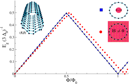
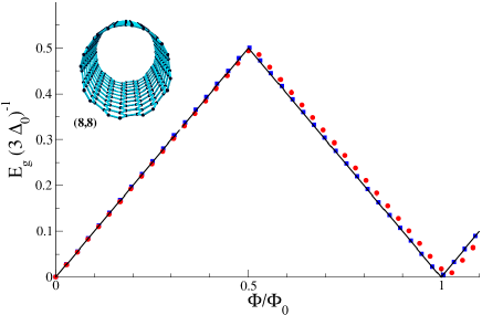
Figure 1: Gap oscillations in the metallic (5,5) and (8,8) CNTs. Two different geometries are considered. In the extended geometry the magnetic field is applied uniformly in all the space (red circles). In the confined geometry , instead, the magnetic field is confined inside the CNT (blue boxes). We compare the ab initio calculations with the ZFA results (black line). We see that in the extended geometry , which represents the standard experimental setup, the Lorentz correction (see text) induces an overestimation of the elemental magnetic flux $\Phi_{0}$.

First we consider two metallic CNTs: a (5,5) tube with radius 6.41 Bohr and a (8,8) tube with radius 10.22 Bohr. In 1 we compare the gap dependence on the applied magnetic flux in the two geometries with the result of the ZFA. In the case of the smaller (5,5) tube we immediately see a first important deviation of the extended geometry from the confined geometry . The extended geometry , which represents the standard experimental setup, overestimates by $\sim$7% the elemental flux $\Phi_{0}$ which defines the periodicity of the gap oscillations. This overestimation of the elemental flux alter the periodicity of gap. Indeed the correction induced in the extended geometry grows with the applied flux. From the dependence of the elemental gap on the applied flux we may deduce that the overall electronic properties of the CNT are still periodic, although with a larger period, in the applied flux. This is not true. As we will discuss later, in the extended geometry a non–periodic correction appears that breaks the periodicity of the gap.

We want, first, to explain the different gap dependence obtained in the two geometries introducing, in a formal manner, the Hamiltonian which governs the AB effect in the specific case of a CNT:

$$H=-\frac{\hbar^{2}}{2m}\left[\frac{\partial^{2}}{\partial r^{2}}+\frac{1}{r}\frac{\partial}{\partial r}+\frac{1}{r^{2}}\left(i\frac{\partial}{\partial\varphi}-\frac{er}{\hbar}A\left(r\right)\right)^{2}+\frac{\partial^{2}}{\partial z^{2}}\right]+V(r,\varphi,z)\text{.}$$ (1)

Eq. 1 describes the electronic dynamics under the action of a static magnetic field, written in cylindrical coordinates centered on the axis of the CNT. $A\left(r\right)$ is the vector potential which, in the symmetric gauge, describes a static magnetic field along the $z$ direction and $V(r,\varphi,z)$ is the local DFT potential, which includes the ionic potential plus the Hartree and exchange–correlation terms.

The only term of Eq. 1 which reflects the different geometry (extended or confined) is $A\left(r\right)$. In the extended geometry

$$A^{extended}\left(r\right)=\frac{1}{2}B_{0}r,$$ (2)

with $B_{0}=\left|{\bf B}\right|$. In the confined geometry , instead, we have that

$$A^{confined}\left(r\right)=\frac{1}{2}\frac{\Phi}{\pi r},$$ (3)

with $\Phi=\pi B_{0}R_{CNT}^{2}$ and $R_{CNT}$ the CNT radius. From Eqs. 2,3 we see that $A^{extended}\left(R_{CNT}\right)=A^{confined}\left(R_{CNT}\right)$, which implies that, if the electrons would exactly move on the tube surface the extended geometry and the confined geometry would lead to the same gap oscillations. The different gap dependence observed in 1, is then due to the quantum nature of the electrons, that can spill out of the tube surface. If we plug the two different expressions for $A\left(r\right)$ into Eq. 1 we get two different Hamiltonians, $H^{confined}$ and $H^{extended}$, whose difference is

$$\Delta H=H^{extended}-H^{confined}=\frac{e\hbar B_{0}}{2m}\left[\left(1-\frac{R_{CNT}^{2}}{r^{2}}\right)i\frac{\partial}{\partial\varphi}+\frac{eB_{0}r^{2}}{4\hbar}\left(1-\frac{R_{CNT}^{4}}{r^{4}}\right)\right]\text{,}$$ (4)

with $\Phi_{0}=h/e$. This term is zero when $r=R_{CNT}$, while near the tube surface behaves like $\sim\left(1-\frac{R_{CNT}^{2}}{r^{2}}\right)$. Now, as shown in 2, the electrons are localized near, but not exactly on the tube surface. Consequently $1-\langle R^{2}_{CNT}/r^{2}\rangle\neq 0$ and, $\langle H^{extended}-H^{confined}\rangle\neq 0$.

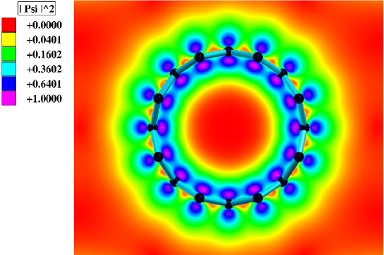
Figure 2: Two dimensional plot of HOMO wave–function at the $\Gamma$ point for the $(8,0)$ CNT. The $\pi$ orbitals, deformed by the curvature of the CNT, have a larger amplitude in the outer part of the CNT surface. As a consequence, in the extended geometry , electrons experience an effective flux which depends on their trajectory, that is not localized on the CNT surface.

We will refer to the correction defined by Eq. 4 as Lorentz Correction (LC) as it introduces a magnetic term which depends on the electronic trajectory (through the term $rA^{extended}_{\phi}$). In the case of pure SWCNTs the LC appears, to first order, as an effective different radius of the electronic orbitals, as the correction would be zero defining the flux with respect to the effective radius which satisfy the equation $1-\langle R^{2}_{eff}/r^{2}\rangle=0$ and so an effective magnetic flux $\Phi^{\prime}$.

From 1 we see that the ZFA matches the ab initio simulation of the standard AB effect corresponding to the confined geometry setup. This agreement is due to the fact that, in the ZFA the LC is strictly zero as the electrons are assumed to move exactly on the graphite sheet, which represents the CNT surface. Consequently in the ZFA the electronic gap is function of the flux only.

Our results reveal that, if the flux is not confined inside the tube the electrons spilled out from the CNT surface can alter the periodicity of the gap oscillations. More importantly the LC can see any deviation of the electron orbital from the perfectly circular surface of the tube. Consequently, even if the LC goes to zero in the case of SW–CNTs with increasing radius, impurities or defects can alter the electronic trajectory creating deviations from a perfect circle of radius $R_{CNT}$. Even in large CNTs. We will see later a particularly large effect of the LC in the case of MWCNTs where bunches of electrons are confined on tubes with different radii.

From 1, we may deduce that the LC increases the elemental flux $\Phi_{0}$ of the gap oscillations, still maintaining the gap periodicity. However this is not true. The gap periodicity is a distinctive feature of the standard AB effect. This is related to the gauge invariance of the theory, that, in the confined geometry follows from the dependence of Eq. 3 on the magnetic flux only. In the extended geometry , instead, Eq. 2 depends on the explicit position of the electron. The LC, therefore, breaks the gauge–invariance of the theory inducing a gap correction that is not periodic in the applied flux.

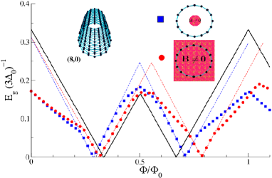
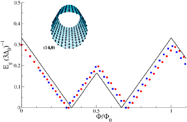
Figure 3: Gap oscillations in a semiconducting CNTs: (8,0) and (14,0). In the extended geometry the magnetic field is applied uniformly in all the space (red circles). In the confined geometry , instead, the magnetic field is confined inside the CNT (blue boxes). We compare the ab initio calculations with the ZFA results (black line). In contrast to the metallic case the curvature effects induce more evident differences between the confined and the extended geometries. In the (8,0) tube the appearance of a metallic band in the gap deeply influences the gap behavior (see text).

We now consider two semi-conducting CNTs: the (8,0) and the (14,0). The flux dependent electronic gap is shown in 3. Similarly to the metallic case, LC makes the extended geometry to oscillate with a period greater than $h/e$. In contrast to the metallic case, the gap vanishes at two values of $\Phi$, which the ZFA predicts to be at $\Phi_{0}/3$ and $2\Phi_{0}/3$, when the Dirac points becomes allowed $k$ points ⁴. Noticeably both points are renormalized in the ab initio simulation by curvature effects. It is well known, indeed, that, compared to graphene, curvature effects shift the Dirac points ⁴ $K$ at a position $|K|<2\pi/3a$, with $2\pi/3a$ the Dirac point position in graphene. Accordingly a lower magnetic field is needed to let the Dirac point belong to the set of the allowed $k$ points and semiconducting CNTs becomes metallic at $\Phi<\Phi_{0}/3$. Being the oscillations symmetric, the second metallic point is reached at $\Phi>2\Phi_{0}/3$.

The deformation of the oscillations in the $(n,0)$ CNTs is smaller in bigger tubes. However it goes to zero slowly because both the shift and the magnetic period depend on the size of the tube. For this reason the effect is still not negligible in the large $(14,0)$ tube as shown in 3.

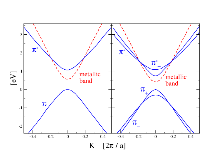
Figure 4: Metallic–like (red dashed line) and $\pi/\pi^{*}$ (blue continuous line) bands of the $(8,0)$ CNT. On the left panel $\Phi=0$, while on the right $\Phi>0$. At finite fluxes the metallic–like band is not split by the breaking of the time reversal symmetry.

From 3 we see that the $(8,0)$ gap oscillations strongly deviate from the ZFA that does not reproduce, even qualitatively, the full ab initio results. The reason for this large discrepancy traces back to the presence of a metallic–like band located near the Fermi surface.

This band is shown in 4 together with the $\pi/\pi^{*}$ bands close to the Fermi level. When the $\mathbf{B}$ field is increased we see that, in contrast to the $\pi/\pi^{*}$ bands, the metallic–like band does not shift, but moves inside the gap. Consequently by changing the flux intensity the gap is defined by transitions between the $\pi/\pi^{*}$ states or between the $\pi$ and the metallic–like band. This explains the anomalous $\Phi$ dependence of $E_{g}$ shown in 3.

Although SW–CNTs are routinely synthesized, MW–CNTs still constitute the majority of cases used in the experiments. In 5 we consider the case of a $(5,5)@(10,10)$ CNT with radii 3.39 and 6.78 Å. In this case the confined geometry is implemented considering the flux $\Phi=\pi B_{0}R_{(10,10)}^{2}$. This flux is roughly the same experienced, in the extended geometry , by the electrons of the $(10,10)$ CNT.

There is here a clear difference between the confined geometry and the extended geometry . The former describes a pure AB effect, where all the electrons feel the same magnetic flux, while in the latter electrons can move on tubes with different radii and it is not possible any more to define a unique magnetic flux. In this case the ZFA can be applied only by considering two different Hamiltonians, one for the $(5,5)$ and one for the $(10,10)$ and by neglecting the tube–tube interaction.

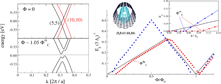
Figure 5: Gap oscillations in a Multi–walled CNT: (5,5)@(10,10) (right frame). Zoom of the metallic intersection of the $\pi/\pi^{*}$ bands at zero and at low flux (left frames). Two different geometries are considered. In the extended geometry the magnetic field is applied uniformly in all the space (red circles). In the confined geometry , instead, the magnetic field is confined inside the CNT (blue boxes). We compare the ab initio calculations with the ZFA results (black line). We immediately see that, in contrast to the ZFA, both geometries are characterized by a metallic phase at low fluxes, highlighted in the inset. The flux which defines the end of the metallic phase is defined as $\Phi^{m}_{c}$. For $\Phi>\Phi^{m}_{c}$ the MW–CNT is an indirect semiconductor. For $\Phi=\Phi^{dg}_{c}$ the tube turns in a direct–gap semiconductor (see text).

The gap calculated in the extended geometry follows the ZFA prediction except in the very low field regime (and near the first inversion point, $\Phi\approx\Phi_{0}$). Moreover, from 5, we notice that, in the confined geometry , $\Phi_{0}$ is $\approx 4\%$ larger then in the ZFA. This renormalization is larger then in the isolated $(10,10)$ SW–CNT that, according to our results, is $<1\%$. This follows from the fact that in the smaller $(8,8)$ tube the renormalization is $\approx 1\%$ and it is expected to further decrease increasing the CNT radius. The reason for the enhancement of the LC in MW–CNTs can be understood by noticing that, in this case, the inner tube attracts the electrons of the outer tube thus increasing the fraction of electronic charge that is spilled out of the tube surface. This phenomena decreases the effective radius felt by the electrons, thus increasing the effect of the LC.

One of the most severe problems that prevent a full investigation of the AB effect in small nano–structures is the need of huge magnetic fields. For example the magnetic field corresponding to the elemental flux of the $(10,10)$ tube is $\approx 2900$ T. Nevertheless the present results suggest possible physical phenomena that can be experimentally observed. We have seen, indeed, that in the simple case of a DW–CNT the existence of an inner tube increases the LC effect by more than a factor 4. Therefore the effect of the LC, although decreasing with increasing tube radius, can be enhanced by altering mechanically the trajectories of the electrons. This is what commonly happens in the case of junctions, defects, dislocations or deformed CNTs. In this last case, for example, an elliptical section of the tube would introduce an angle $\phi$ dependence in Eq.4. This would contribute to the breaking of the gauge–invariance, thus enhancing the LC.

Another phenomena, predicted by the present ab initio calculations, that can be experimentally investigated, is the metallic regime for $\Phi\leq\Phi^{m}_{c}$ observed in MW–CNTs. This regime can be described only by using a TBM with ad–hoc parameters included, a posteriori, to mimic the tube–tube interaction ¹⁷. The present scheme, instead, in a parameter–free manner, predicts a metallic phase and, in addition, a transition from an indirect to a direct semi–conductive phase. The metallic phase is a consequence of the different chemical potential felt by the electrons moving on the $(5,5)$ and the $(10,10)$ surfaces. The ab initio calculations shows that there is a $\approx 0.09eV$ shift between the two chemical potentials, as shown in 5 (left frames), where the band structure of the tube is shown at $\Phi=0$ (upper frame), and at $\Phi\approx 1.1\Phi^{m}_{c}$ (lower frame).

At zero magnetic flux we see two pairs of crossing bands which can be identified as the $\pi-\pi^{*}$ bands of the $(5,5)$ and the $(10,10)$ CNTs respectively. The two crossing points are not aligned in energy so that when a magnetic flux is applied two small direct gap opens but the CNT remains metallic as long as the tip of the $\pi^{*}$ band of the $(5,5)$ is lower in energy than the one of the $\pi$ band of the $(10,10)$ CNT. Only when $\Phi=\Phi^{m}_{c}$ a gap opens and the system turns in an indirect–gap semiconductor, where the last occupied is a $\pi$ band of the outer (10,10) tube, while the first unoccupied is a $\pi^{*}$ band of the inner (5,5) tube.

From the right frame of 5 we also notice a sudden change in the gap velocity ¹⁸, defined as $v_{g}\left(\Phi\right)=\frac{1}{\mu_{B}}\frac{dE(B)}{dB}$, when $\Phi=\Phi^{dg}_{c}$. At this flux the MWCNT turns in a direct–gap semiconductor, while for $\Phi<\Phi^{dg}_{c}$ the tube is an indirect–gap semiconductor. This happens because the $\pi$ band of the (10,10) tube moves faster than the $\pi$ band of the (5,5) tube. At $\Phi=\Phi^{dg}_{c}$ the relative ordering of the two bands is inverted and the gap is determined by the $(5,5)$ $\pi-\pi^{*}$ bands, thus recovering the prediction of the ZFA.

The critical field $\Phi^{m}_{c}$ represents, experimentally, an accessible flux regime. Indeed from our ab initio approach $B^{m}_{c}\approx 180$ T for the $(5,5)@(10,10)$. By using the dependence of the electronic properties of the CNTs on the radius¹⁹ we can extrapolate, for example, $B^{m}_{c}\approx 20$ T for a $(10,10)@(15,15)$ MW–CNT.

We have discussed the metal–semiconductor transition induced by the magnetic field in the maximally symmetric geometry of an ideally isolated (n,n)@(m,m) CNT. Nevertheless the effect on the electronic properties of the tube–tube interaction and of a different relative orientation of the two CNTs that compose the DW–CNT is known from both ab–initio simulations ^{20, 21} and TB model results ^{10, 17}. Calculations performed by using the TB model on the (5,5)@(10,10) CNT ¹⁰ show that the main effect is the appearance of four pseudo–gaps. Nevertheless, the tube remains metallic due to the shift in the chemical potential, and the behavior of the electronic states perturbed by the external magnetic flux is not modified ¹⁷. Therefore the overall effect of the tube–tube interaction and of the different relative angular orientation of the two CNTs would be a shortening of the metallic phase. This corresponds to a reduction of the critical flux even below the one we have predicted for the ideal DW–CNT

In conclusion, using an ab initio approach, we have predicted that the gap of SW and MW–CNTs interacting with a magnetic field is characterized by anomalous Aharonov–Bohm oscillations. In the standard experimental setup, when the CNT is fully immersed in a uniform magnetic field, the gap oscillations cannot be interpreted in terms of the standard Aharonov–Bohm effect. Also in the case of a really confined magnetic field the quantum nature of the electrons induce corrections to the pure Aharonov–Bohm oscillations. Curvature effects and metallic bands have been shown to induce an anomalous dependence of the gap on the applied flux, not predicted by the state–of–the–art theory based on the Zone Folding approach. The quantum delocalization of the electronic wave–functions has been shown to induce classical Lorentz Corrections that break the periodicity of the gap. In MW–CNTs we have predicted the existence of metallic, indirect–gap and direct–gap semi–conductive phases with the length of the metallic phase directly connected to the geometry of the applied field. We have also discussed how this metallic phase can be measured by using realistically weak magnetic fields, and how the Lorentz correction can appear, in the extended geometry , any time a dislocation, a defect or a tube deformation alter the circular trajectory of the electrons.

The present results do contribute to improve the state–of–the–art understanding of the Aharonov–Bohm effect at the nano–scale. They clearly bind a quantitative description of the gap oscillations induced by a magnetic flux to a careful inclusion of quantum effects on the electronic trajectories and to an ab initio , parameter–free description of the nano–tube electronic states.

This work was supported by the EU through the FP6 Nanoquanta NoE (NMP4-CT-2004-50019), the FP7 ETSF I3 e-Infrastructure (Grant Agreement 11956). One of the authors (AM) would like to acknowledge support from the HPC-Europa2 Transnational collaboration project. One of the authors (DS) would like to thank prof. Giovanni Onida and prof. Angel Rubio for supporting this work and for useful discussions and suggestions.

References

- Aharonov and Bohm 1959 Aharonov, Y.; Bohm, D. Phys. Rev. 1959, 115, 485–491
- Chambers 1960 Chambers, R. G. Phys. Rev. Lett. 1960, 5, 3–5
- Tonomura et al. 1986 Tonomura, A.; Osakabe, N.; Matsuda, T.; Kawasaki, T.; Endo, J. Phys. Rev. Lett. 1986, 56, 792–795
- Charlier et al. 2007 Charlier, J.-C.; Blase, X.; Roche, S. Rev. Mod. Phys. 2007, 79, 677–732
- Bachtold et al. 1999 Bachtold, A.; Strunk, C.; Salvetat, J. P.; Bonard, J. M.; Forro, L.; Nussbaumer, T.; Schonenberger, C. Nature 1999, 397, 673–675
- Abrahams et al. 1979 Abrahams, E.; Anderson, P. W.; Licciardello, D. C.; Ramakrishnan, T. V. Phys. Rev. Lett. 1979, 42, 673–676
- Al’tshuler et al. 1981 Al’tshuler, B. L.; Aronov, A. G.; Spivak, B. Z. Pis’ma Zh. Eksp. Teor. Fiz. 1981, 33, 101–103
- Coskun et al. 2004 Coskun, U. C.; Wei, T.; Vishveshwara, S.; Goldbart, P. M.; Bezryadin, A. Science 2004, 304, 1132–1134
- Zaric et al. 2004 Zaric, S.; Ostojic, G. N.; Kono, J.; Shaver, J.; Moore, V. C.; Strano, M. S.; Hauge, R. H.; Smalley, R. E.; Wei, X. Science 2004, 304, 1129–1131
- Kwon and D. 1998 Kwon, Y.-K.; D., T. Physical Review B 1998, 58, R16001
- Goedecker et al. 1996 Goedecker, S.; Teter, M.; Huetter, J. Phys. Rev. B 1996, 54, 1703
- 12 The ground state calculations were performed using a plane–wave basis and norm–conserving Troullier–Martins pseudopotentials. The kinetic energy cut–off used is Ha. The Brillouin zone was sampled using k–points grids aligned with the tube axis. After carefull convergence tests we used k–points (in the irreduceble Brillouin Zone) for the , k–points for the and k–points for the CNT. Only for the CNT the elemental gap was calculated by using more refined k–point grids in the non self–consistent calculation.
- Marini et al. 2009 Marini, A.; Hogan, C.; Grüning, M.; Varsano, D. Comp. Phys. Comm. 2009, 180, 1392–1403
- 14 In particular we used Eq. 9 of Ref. 22.
- 15 yambo diagonalizes self–consistently the Hamiltonian in the basis–set of the KS–wavefunctions at zero magnetic field. On average we need to include at least 50 (up to 100) conduction bands in order to obtain a converged gap up to . Moreover, to improve convergence yambotakes advantage of gauge freedom in the choice of the vector potential.
- 16 The confined geometry is commonly used to model the AB effect. However an extended geometry has been used, for example, to describe the effect of quantum confinement induced by strong magnetic fields23.
- Latge and Grimm 2007 Latge, A.; Grimm, D. Carbon 2007, 45, 1905–1910
- 18 The Bohr magneton eV/T is introduced in order to make dimensionless.
- 19 The critical magnetic field depends on the ratio with the shift of the chemical potential with respect to an ideal tube with . This is a curvature induced effect and it is expected 24 to be . As the maximum gap 4 of a CNT during an AB oscillation is proportional to and one oscillation must be completed when one can obtain . From our ab initio simulation of the CNT we know that T and eV. Thus we obtain , , eV and eV. Finally, using these values we can infer that T for a CNT.
- Charlier and Michenaud 1993 Charlier, J.; Michenaud, J. Physical Review Letters 1993, 70, 1858
- 21 However, only recently, new DFT functionals have been proposed to correctly describe the Van Der Waals component of the tube–tube interaction 25.
- Pickard and Mauri 2003 Pickard, C. J.; Mauri, F. Phys. Rev. Lett. 2003, 91, 196401
- Ferrari et al. 2009 Ferrari, G.; Goldoni, G.; Bertoni, A.; Cuoghi, G.; Molinari, E. Nano Letters 2009, 9, 1631–1635
- Kane and Mele 1997 Kane, C. L.; Mele, E. J. Phys. Rev. Lett. 1997, 78, 1932
- Romàn-Pèrez and Soler 2009 Romàn-Pèrez, G.; Soler, J. M. Physical Review Letters 2009, 103, 096102