Metric Deformation and Boundary Value Problems in 2D

Abstract

A new analytical formulation is prescribed to solve the Helmholtz equation in 2D with arbitrary boundary. A suitable diffeomorphism is used to annul the asymmetries in the boundary by mapping it into an equivalent circle. This results in a modification of the metric in the interior of the region and manifests itself in the appearance of new source terms in the original homogeneous equation. The modified equation is then solved perturbatively. At each order the general solution is written in a closed form irrespective of boundary conditions. This method allows one to retain the simple form of the boundary condition at the cost of complicating the original equation. When compared with numerical results the formulation is seen to work reasonably well even for boundaries with large deviations from a circle. The Fourier representation of the boundary ensures the convergence of the perturbation series.

1 Introduction

The two dimensional Helmholtz equation appears in a wide range of physical and engineering problems across diverse fields $-$ like the study of vibration, acoustic and electromagnetic (EM) wave propagation and quantum mechanics. In a large class of these problems one is required to determine the eigenspectrum of the Helmholtz operator for various boundary conditions and geometries. Canonical examples of the Dirichlet boundary condition (DBC) are the vibration of membranes, the propagation of the TM modes of EM waves within a waveguide and a quantum particle confined in an infinite deep potential well. Perhaps the prominent example of the Neumann boundary condition (NBC) is the transmission of the TE modes of EM waves in a waveguide. Analytic closed-form solution to the boundary value problems [1, 2, 3] can however be obtained only for a restricted class of boundaries. The problem for rectangular, circular, elliptical and triangular boundaries are classical ones addressed by Poisson, Clebsch, Mathieu and Lamé respectively [1]. Invoking the geometry of the problem by a suitable choice of co-ordinates often aids in finding the solutions (e.g. elliptic boundary where, separation of variables leads to a solution in the form of Mathieu functions). However, one quickly exhausts the list of such problems where simplification by virtue of using a specific co-ordinate system is possible. In most physical problems, one encounters boundaries which are far removed from such idealization like the case of the quantum dot. The dots are believed to be circular but in practice that can hardly be guaranteed [4, 5, 6, 7]. In such a scenario it is natural to consider the confining region to be a supercircle [8]. Another important deviation from such idealization is the design of waveguides with a shape, other than a rectangular or a circular, that can be handy to purge the losses due to corners [9]. Further, the problem gets analytically intractable for arbitrary boundaries. The study of propagation of the electromagnetic waves in open dielectric systems for an arbitrary cross-section has been studied recently [10].

The problem of solving Helmholtz equation for an arbitrary boundary has mostly been tackled using numerical methods [11, 12, 13, 14, 15, 16, 17, 18, 20, 21, 23, 24, 19, 22]. The analytic approach towards this has mainly revolved around various approximation methods. Of these, the perturbative techniques stand out as being the most widely used [1, 2, 3, 24, 25, 27, 28, 29, 30, 26], where the starting point is the Rayleigh's theorem : which states that the gravest tone of a membrane whose boundary has slight departure from a circle, is nearly the same as that of a mechanically similar membrane in the form of a circle of the same mean radius or area. For slight departure from circular boundary, one expands the wavefunction in terms of a complete set of eigenfunctions (viz. Bessel functions) of the unperturbed case (i.e. a circular boundary). Then the wavefunction is made to satisfy the given condition on the arbitrary boundary and which in turn extracts out the expansion coefficients of the required wavefunction. The works [3, 30, 31, 32, 33] study arbitrary domains in a general formalism using Fourier representation of the boundary asymmetry treated as a perturbation around an equivalent circle. In contrast ref. [24] studies analytic methods where the arbitrary simply connected domain is mapped to a square by conformal mapping and then the eigenvalues are approximated order by order in the basis of a square boundary. In ref. [24] the zeros of Bessel functions are approximated (i.e. energy eigenvalues associated with a unit radius circle) from a square box. In our case we have approximated the eigenvalues associated with a square box from an equivalent circle. The ref. [24] has done a perturbation up to the third order whereas in our case we have done up to first order except the cases for $l=0$ states where the second order corrections are also included. It can be easily seen from the respective tables (Table III in ref. [24] and Table I in our paper) that at the first order, both the methods have comparable efficiency. Ref. [24] focuses its attention mainly towards the eigenvalues in case of Dirichlet boundary condition, whereas our formulation in a single stroke handles Neumann condition as well. Moreover our paper gives at each order of perturbation the correction to the wavefunction exactly. We have also written down the exact expression for the $n^{\rm{th}}$ order correction to the eigenvalue in abstract sense.

We have explored an alternative approach towards solving the eigenvalue problem for the two dimensional Helmholtz operator in the interior of a region bounded by an arbitrary closed curve. The general problem is mapped into an equivalent problem where the boundary is a regular closed curve (for which the Helmholtz equation is exactly solvable) whereas the equation itself gets modified owing to the deformation of the metric in the interior. The modified equation, we see, can be written as the original Helmholtz equation with additional terms arising from transformation in the metric. The extra pieces can now be treated as a perturbation to the original Helmholtz operator. The equation is thereby solved using the Schrödinger perturbation technique [34]. The corrections to the eigenfunctions are expressed in a closed form at each order of perturbation irrespective of boundary condition. The eigenvalue corrections are then obtained by imposing the appropriate boundary condition. This is in contrast to the earlier methods where the formulations are generally boundary condition dependent. In this approach towards solving the equation, the boundary conditions are specified on some known regular curve and maintain the same simple form at each order of perturbation. This bypasses the issue of imposing constraints on a boundary having a complicated geometry [31, 32, 33].

We expect this perturbative scheme to effectively solve the eigenvalue problem for boundaries which reflect slight departure from known regular curves. We have verified our method against the numerically obtained solutions for a supercircle and an ellipse. In this analysis we use Fourier representation of the boundary. This allows us to apply the method to a general class of continuous or discontinuous asymmetries. Section 2 describes the general formalism in abstract sense. In section 3, we deal with the non degenerate case ($l=0$) and find solutions up to second order. Section 4 tackles the degenerate case ($l\neq 0$) and obtains the first order correction to energy and eigenfunction. In section 5, we apply the method for supercircular and elliptical boundaries and compare our analytic perturbative results with the numerically obtained ones. Finally, we summarise our results noting the advantages of our method over the other existing ones and conclude with a few comments.

2 Formulation

The homogeneous Helmholtz equation on a 2 dimensional flat simply connected surface $\cal S$ reads,

$$\left(g_{ij}\nabla^{i}\nabla^{j}+k^{2}\right)\psi\equiv\left(\nabla^{2}+E\right)\psi=0,$$ (1)

where $g_{ij}$ is the flat metric and $\nabla$ represents a covariant derivative. We look for solutions in the interior of the bounded region with the Dirichlet condition $\psi=0$ or the Neumann condition $\frac{\partial\psi}{\partial n}=0$ on $\partial\cal S$, where $\frac{\partial\psi}{\partial n}$ denotes the derivative along the normal direction to $\partial\cal S$. The parameter $k^{2}$ may be identified with $E$, the energy of a quantum particle confined in the region having a boundary $\partial\cal S$.

It is convenient to work in polar coordinate system ($r,\theta$), where any closed curve satisfies the periodicity condition $r(\theta)=r(\theta+2\pi)$. We consider a general arbitrary boundary of the form $r=r(\theta)$. In this analysis we assume that the arbitrary boundary can be expressed as a perturbation around an effective circle (the analysis can in principle work for a deformation around any simple curve for which the Helmholtz equation is exactly solvable). We introduce new coordinates $(R,\alpha)$ with the transformation $(r,\theta)\rightarrow(R,\alpha)$ given by

$$\begin{split}r=~{}&R+\epsilon f(R,\alpha)~{};\\ \theta=~{}&\alpha~{},\end{split}$$ (2)

where $\epsilon$ is a deformation parameter. This defines a diffeomorphism for the entire class of well behaved functions $f(R,\alpha)$. A suitable choice of $f(R,\alpha)$, shall transform our arbitrary boundary into a circle of average radius, say $R_{0}\,(=\frac{1}{2\pi}\int\limits^{2\pi}_{0}r(\theta)\,\,\text{d}\theta)$ in the $R-\alpha$ plane. The deformation of the arbitrary boundary to a circle changes the components of the underlying metric $g_{ij}(r,\theta)$ in the interior ($g_{ij}(r,\theta)\rightarrow\tilde{g}_{ij}(R,\alpha)$). Henceforth, we use the notation

$$\phi^{(i,j)}\equiv\frac{\partial^{i+j}\phi}{\partial R^{i}\partial\alpha^{j}}~{},$$

where $\phi$ is a function of $R$ and $\alpha$. The dependence on the arguments $(R,\alpha)$ are not shown explicitly for brevity. The flat background metric in the ($r,\theta$) system is given by $g_{ij}={\rm diag}(1,r^{2})$. Under the coordinate transformations (2) this takes the form

$$\tilde{g}_{ij}=\left[\begin{array}[]{ll}\quad\left(1+\epsilon f^{(1,0)}\right)^{2}\qquad\quad\,\,\,~{}\epsilon f^{(0,1)}\left(1+\epsilon f^{(1,0)}\right)\\ \epsilon f^{(0,1)}\left(1+\epsilon f^{(1,0)}\right)\qquad(R+\epsilon f)^{2}+\epsilon^{2}f^{{(0,1)}^{2}}\end{array}\right],$$

We note that except for $\Gamma^{\alpha}_{{\phantom{\alpha}}RR}$ all the components of connection $\Gamma$ are non-vanishing. The diffeomorphism (2) does not induce any spurious curvature in the manifold (i.e. Riemann tensor, $R^{i}_{{\phantom{i}}jkl}=0~{}~{}\forall~{}i,j,k,l$).

The Eq. (1), where $\psi=\psi(r,\theta)$, transforms under the map $(r,\theta)\rightarrow(R,\alpha)$ to

$$E~{}\psi+\frac{\psi^{(0,2)}}{(R+\epsilon f)^{2}}+\frac{\left[(R+\epsilon f)^{2}-\epsilon f^{(0,2)}\left(R+\epsilon f\right)+2\epsilon^{2}f^{{(0,1)}^{2}}\right]\psi^{(1,0)}}{(R+\epsilon f)^{3}\left(\epsilon f^{(1,0)}+1\right)}$$

$$+\frac{2\epsilon^{2}f^{(0,1)}\left[(R+\epsilon f)f^{(1,1)}-f^{(0,1)}\left(\epsilon f^{(1,0)}+1\right)\right]\psi^{(1,0)}}{(R+\epsilon f)^{3}\left(\epsilon f^{(1,0)}+1\right)^{2}}-\frac{2\epsilon f^{(0,1)}\psi^{(1,1)}}{(R+\epsilon f)^{2}\left(\epsilon f^{(1,0)}+1\right)}$$

$$-\frac{\epsilon f^{(2,0)}\left[(R+\epsilon f)^{2}+\epsilon^{2}f^{{(0,1)}^{2}}\right]\psi^{(1,0)}}{(R+\epsilon f)^{2}\left(\epsilon f^{(1,0)}+1\right)^{3}}+\frac{\left[(R+\epsilon f)^{2}+\epsilon^{2}f^{{(0,1)}^{2}}\right]\psi^{(2,0)}}{(R+\epsilon f)^{2}\left(\epsilon f^{(1,0)}+1\right)^{2}}=0\,.$$ (3)

The analysis can proceed from here for a specific form of the function $f(R,\alpha)$. We choose $f(R,\alpha)=Rg(\alpha)$, where $g(\alpha)$ can be expanded without a loss of generality in a Fourier series. We further impose $g(\alpha)=g(-\alpha)$ for simplicity whereby only the cosine terms are retained

$$g(\alpha)=\sum_{n=1}^{\infty}C_{n}\cos n\alpha.$$ (4)

The constant part $C_{0}$ can always be absorbed in $R$ defined in (2). With this choice of $f(R,\alpha)$, Eq. (2) simplifies to

$$\sum_{n=0}^{\infty}\epsilon^{n}{\cal L}_{n}\psi+E\psi=0,$$ (5)

where the operator ${\cal L}_{n}$ is given by

$${\cal L}_{n}\psi=(-1)^{n}\frac{(n+1)}{6R^{2}}g^{n-2}\left[3nRg\left\{g^{(0,2)}\psi^{(1,0)}+2g^{(0,1)}\psi^{(1,1)}\right\}\right.$$ (6)

$$\left.\quad+n(n-1)R\left(g^{(0,1)}\right)^{2}\left\{2\psi^{(1,0)}+R\psi^{(2,0)}\right\}+6g^{2}\left\{\psi^{(0,2)}+R\psi^{(1,0)}+R^{2}\psi^{(2,0)}\right\}\right].$$

We shall adopt the method of stationary perturbation theory [34] to solve for $\psi$ and $E$. Thereby, treating $\epsilon$ as a perturbation parameter we expand the eigenfunction $\psi$ corresponding to the eigenvalue $E$ as

$$\psi =\psi^{(0)}+\epsilon\psi^{(1)}+\epsilon^{2}\psi^{(2)}+\cdots;$$ (7a)

$$E =E^{(0)}+\epsilon E^{(1)}+\epsilon^{2}E^{(2)}+\cdots,$$ (7b)

with superscripts denoting the order of perturbation. We assume that the perturbative scheme converges and $(\psi,E)$ can be calculated order by order up to any arbitrarily desired precision. We note that the parameter $\epsilon$ is arbitrarily invoked to track different orders and could be absorbed in the Fourier coefficients $C_{n}$.

Plugging (7) in (5), and collecting the coefficients for different powers of $\epsilon$ yields

$${\mathcal{O}}(\epsilon^{0}) : ({\cal L}_{0}+E^{(0)})\psi^{(0)}=0~{},$$ (8a)

$${\mathcal{O}}(\epsilon^{1}) : ({\cal L}_{0}+E^{(0)})\psi^{(1)}+({\cal L}_{1}+E^{(1)})\psi^{(0)}=0~{},$$ (8b)

$${\mathcal{O}}(\epsilon^{2}) : ({\cal L}_{0}+E^{(0)})\psi^{(2)}+({\cal L}_{1}+E^{(1)})\psi^{(1)}+({\cal L}_{2}+E^{(2)})\psi^{(0)}=0~{},$$ (8c)

$$\vdots$$

$${\mathcal{O}}(\epsilon^{m}) : \sum_{n=0}^{m}\left({\cal L}_{n}+E^{(n)}\right)\psi^{(m-n)}=0~{}.$$ (8d)

The change in the metric components induced by the smooth deformation (2) amounts to a gauge transformation and generates source terms to the unperturbed homogeneous Helmholtz equation at each order in $\epsilon$. At the $i^{\text{th}}$ order we have the terms ${\cal L}_{1}\psi^{(0)},\,{\cal L}_{1}\psi^{(1)},\,\cdots,\,{\cal L}_{i}\psi^{(j(<i))}$, which have no physical origin and are merely artifacts of the chosen gauge. Maintaining the simplicity of the boundary conditions is hence achieved at the cost of new terms appearing in the original equation.

The unperturbed energy $E^{(0)}$ and corrections $E^{(1)}$, $E^{(2)}$ are given by

$$E^{(0)}= -\langle\psi^{(0)}|{\cal L}_{0}|\psi^{(0)}\rangle;$$ (9a)

$$E^{(1)}= -\langle\psi^{(0)}|{\cal L}_{1}|\psi^{(0)}\rangle;$$ (9b)

$$E^{(2)}= -\langle\psi^{(0)}|{\cal L}_{1}+E^{(1)}|\psi^{(1)}\rangle-\langle\psi^{(0)}|{\cal L}_{2}|\psi^{(0)}\rangle.$$ (9c)

$$\vdots$$

$$E^{(m)}= -\Big{\langle}\psi^{(0)}\Bigl{\lvert}\sum_{n=1}^{m-1}\left({\cal L}_{n}+E^{(n)}\right)\Bigr{\rvert}\psi^{(m-n)}\Big{\rangle}-\Big{\langle}\psi^{(0)}\Bigl{\lvert}{\cal L}_{m}\Bigr{\rvert}\psi^{(0)}\Big{\rangle}.$$ (9d)

A unique feature of our method is that both the boundary conditions maintain their simple forms separately for every order in perturbation. Thus, we have for the $i^{\text{th}}$ order wavefunction the DBC and the NBC respectively,

$$~{}\psi^{(i)}(R_{0},\alpha)=0\,,\qquad\qquad\qquad\qquad\quad\qquad~{}\mbox{(DBC)}\,;$$ (10a)

$$\left(\frac{\partial\psi^{(i)}}{\partial R}-\frac{g^{(0,1)}}{R}\frac{\partial\psi^{(i-1)}}{\partial\alpha}\right)\Bigg{\rvert}_{(R_{0},\alpha)}=0\,,\quad\quad~{}\mbox{(NBC)}\,,$$ (10b)

where $i\in\mathbb{N}$. The general solution of the Eq. (8a) is

$$\psi_{l,j}^{(0)} =N_{0,j}J_{0}(\rho)\,,\qquad\qquad\qquad\qquad~{}(l=0)\,;$$

$$=N_{l,j}J_{l}(\rho)\left\{\begin{array}[]{c}\cos(l\alpha)\\ \sin(l\alpha)\end{array}\right\},\qquad\quad(l\neq 0)\,,$$ (13)

where $J_{l}$ is the $l^{\text{th}}$ order Bessel function with the argument $\rho=\sqrt{E_{l,j}^{(0)}}R$, where $E_{l,j}^{(0)}$ are the energies of the unperturbed Helmholtz equation. $N_{l,j}$ is a suitable normalisation constant with $l\in\mathbb{N}$, $j\in\mathbb{N}_{>0}$. It is to be noted that the normalisation constant will be different for the different boundary conditions. Henceforth, we will discuss both the cases, viz. the Dirichlet and the Neumann boundary condition parallely. The energy $E_{l,j}^{(0)}$ is dictated by the $j^{\text{th}}$ zero of $J_{l}$, denoted by $\rho_{{}_{l,j}}$, and the $j^{\text{th}}$ zero of $J^{\prime}_{l}$, denoted by $\rho^{\prime}_{{}_{l,j}}$, for DBC and NBC respectively. Using Eq. (10a) and (10b) for $i=0$, we have

$$E_{l,j}^{(0)}=~{} \rho^{2}_{{}_{l,j}}/R_{0}^{2}\,,~{}\qquad\qquad\mathrm{(DBC)}~{};$$ (14)

$$=~{} \rho^{\prime^{2}}_{{}_{l,j}}/R_{0}^{2}\,,\qquad\qquad~{}\mathrm{(NBC)}~{},$$ (15)

where all the levels with non-zero $l$ are doubly degenerate.

In this formulation the energy corrections can be obtained in two ways. Firstly, $E^{(i)}$ can be estimated from the knowledge of $\psi^{(m)}(\forall~{}m<i)$ using Eqs. (9). Alternatively it can be extracted by imposing the boundary condition on $\psi^{(i)}$ given by Eqs. (10), which in addition yields the coefficients of Bessel functions (in $\psi^{(i)}$). The method can in principle be used to calculate corrections at all orders of perturbation. We next calculate the energy corrections for both the boundary conditions for the following two cases.

3 Case I: Non-degenerate states ($l=0$)

The first order correction to the eigenfunction is obtained solving the Eq. (8b). Thus, we have

$$\psi_{0,j}^{(1)}= \,a_{0}J_{0}(\rho)-\frac{\rho E_{0,j}^{(1)}}{2E_{0,j}^{(0)}}N_{0,j}J_{1}(\rho)+\sum_{p=1}^{\infty}{\Big{\{}}a_{p}J_{p}(\rho)-\rho N_{0,j}C_{p}J_{1}(\rho){\Big{\}}}\cos(p\alpha),$$ (16)

where $E_{0,j}^{(1)}$, $a_{0}$ and $a_{p}$ are constants to be fixed by the boundary conditions. The terms contain $N_{0,j}J_{1}(\rho)$ make the particular integral of the Eq. (8b). The first order energy corrections are obtained by imposing the respective boundary condition, given by Eq. (10a) or by substituting $\psi_{0,j}^{(1)}$ and $\psi_{0,j}^{(0)}$ into the Eq. (10b), (for $i=1$). This yields

$$E_{0,j}^{(1)}=0~{}~{}~{}\mbox{(for both the cases)};$$

$$a_{p}=\rho_{{}_{0,j}}N_{0,j}C_{p}J_{1}(\rho_{{}_{0,j}})/J_{p}(\rho_{{}_{0,j}})\,,~{}(p\neq 0)~{}\mbox{(DBC)};$$

$$a_{p}=\rho^{\prime}_{{}_{0,j}}N_{0,j}C_{p}J_{0}(\rho^{\prime}_{{}_{0,j}})/J^{\prime}_{p}(\rho^{\prime}_{{}_{0,j}})\,,~{}(p\neq 0)~{}\mbox{(NBC)}.$$

The vanishing of the first order correction, $E_{0,j}^{(1)}$, is verified using Eq. (9b). The remaining constant $a_{0}$ of Eq. (16) is zero for both the boundary conditions by virtue of orthogonality of $\psi_{0,j}^{(0)}$ and $\psi_{0,j}^{(1)}$. These results are consistent with the results obtained in [31, 32, 33] by other methods.

The first non-vanishing energy correction occurs at the second order. The correction $E_{0,j}^{(2)}$ is obtained by substituting $\psi_{0,j}^{(0)}$ and $\psi_{0,j}^{(1)}$ in Eq. (9c) and have

$$E_{0,j}^{(2)}=E_{0,j}^{(0)}\sum_{n=1}^{\infty}\xi_{n,j}C^{2}_{n}\,;~{}~{}\xi_{n,j}=\frac{1}{2}+\frac{\rho_{{}_{0,j}}J^{\prime}_{n}(\rho_{{}_{0,j}})}{J_{n}(\rho_{{}_{0,j}})},$$ (17)

and

$$E_{0,j}^{(2)}=-\,E_{0,j}^{(0)}\sum_{n=1}^{\infty}\lambda_{n,j}C^{2}_{n}\,;~{}\lambda_{n,j}=\frac{1}{2}+\frac{\rho^{\prime}_{{}_{0,j}}J_{n}(\rho^{\prime}_{{}_{0,j}})}{J^{\prime}_{n}(\rho^{\prime}_{{}_{0,j}})},$$ (18)

for the DBC and the NBC respectively. We may as well solve (8c) to obtain

$$\psi_{0,j}^{(2)}=b_{0}J_{0}(\rho)-\frac{\rho E_{0,j}^{(2)}}{2E_{0,j}^{(0)}}N_{0,j}J_{1}(\rho)+\sum_{n=1}^{\infty}C_{n}{\cal J}_{n,j}(\rho)$$

$$+\sum_{p=1}^{\infty}{\Big{\{}}b_{p}J_{p}(\rho)-\rho a_{0}C_{p}J_{1}(\rho)+\sum_{n=1}^{\infty}\left(C_{n+p}+C_{|n-p|}\right){\cal J}_{n,j}(\rho){\Big{\}}}\cos(p\alpha)\,,$$ (19)

where

$${\cal J}_{n,j}(\rho)=\frac{\rho}{2}{\Big{\{}}a_{n}J^{\prime}_{n}(\rho)-\frac{\rho}{2}N_{0,j}C_{n}J^{\prime}_{1}(\rho){\Big{\}}}.$$

Boundary conditions, Eqs. (10) (for $i=2$), extract $E_{0,j}^{(2)}$ as given in Eq. (17) or Eq. (18) and in addition the coefficients $b_{p}$ are respectively given by

$$b_{p}= ~{}\frac{\rho_{{}_{0,j}}J_{1}(\rho_{{}_{0,j}})}{J_{p}(\rho_{{}_{0,j}})}\left\{a_{0}C_{p}-\frac{N_{0,j}}{2}\sum_{n=1}^{\infty}C_{n}(C_{n+p}+C_{|n-p|})\xi_{n,j}\right\},~{}~{}~{}\mbox{(DBC)};~{}$$

$$= ~{}\frac{\rho^{\prime}_{{}_{0,j}}J_{0}(\rho^{\prime}_{{}_{0,j}})}{J^{\prime}_{p}(\rho^{\prime}_{{}_{0,j}})}\left\{a_{0}C_{p}+\frac{N_{0,j}}{2\rho^{\prime}_{{}_{0,j}}}\sum_{n=1}^{\infty}np\,C_{n}(C_{n+p}-C_{|n-p|})\right.$$

$$\left.\qquad\qquad\qquad\qquad+\frac{N_{0,j}}{2}\sum_{n=1}^{\infty}C_{n}(C_{n+p}+C_{|n-p|})\lambda_{n,j}\right\},~{}~{}~{}~{}\mbox{(NBC)}.$$

The remaining constant $b_{0}$ can be fixed by normalising the corrected wavefunction.

4 Case II: Degenerate states ($l\neq 0$)

In the $l\neq 0$ case, the first order wavefunction correction is given by

$$\psi_{l,j}^{(1)}=\,a_{0}J_{0}(\rho)+\frac{\rho N_{l,j}C_{l}}{2}J^{\prime}_{l}(\rho)+\left\{a_{l}J_{l}(\rho)+\frac{\rho N_{l,j}J^{\prime}_{l}(\rho)}{2}\left(C_{2l}+\frac{E_{l,j}^{(1)}}{E_{l,j}^{(0)}}\right)\right\}\cos(l\alpha)$$

$$\qquad\qquad+\sum_{\begin{subarray}{c}p=1\\ p\neq l\end{subarray}}^{\infty}\left\{a_{p}J_{p}(\rho)+\frac{\rho}{2}N_{l,j}J^{\prime}_{l}(\rho)\left(C_{l+p}+C_{|l-p|}\right)\right\}\cos(p\alpha).$$ (20)

Here we have considered only the `cosine' form of $\psi_{l,j}^{(0)}$ (see Eq. (13)) for the $l\neq 0$ case. The other solution with the $\sin(l\alpha)$ term can be treated similarly. We have estimated the first order energy corrections by imposing the respective boundary conditions for $i=1$ given in Eqs. (10). $E_{l,j}^{(1)}$ is also verified by substituting $\psi_{l,j}^{(0)}$ in Eq. (9b). We have

$$E_{l,j}^{(1)}= -E_{l,j}^{(0)}C_{2l}~{},~{}\qquad\qquad\qquad\qquad\mbox{(DBC)}~{};$$

$$E_{l,j}^{(1)}= -E_{l,j}^{(0)}C_{2l}\left(\frac{\rho^{\prime^{2}}_{{}_{l,j}}+l^{2}}{\rho^{\prime^{2}}_{{}_{l,j}}-l^{2}}\right)~{},~{}~{}~{}\qquad\mbox{(NBC)}~{},$$

where the corresponding $E_{l,j}^{(0)}$ are given by Eq. (14) and Eq. (15) respectively. This is generally non-vanishing unlike the earlier case. The second order energy correction becomes crucial when $C_{2l}=0$. The choice of the `sine' solution for $\psi_{l,j}^{(0)}$ (Eq. 13) gives

$$E_{l,j}^{(1)}= ~{}E_{l,j}^{(0)}C_{2l}~{},\qquad\qquad\qquad\quad\mbox{(DBC)}~{};$$

$$E_{l,j}^{(1)}= ~{}E_{l,j}^{(0)}C_{2l}\left(\frac{\rho^{\prime^{2}}_{{}_{l,j}}+l^{2}}{\rho^{\prime^{2}}_{{}_{l,j}}-l^{2}}\right)~{},~{}~{}\quad\mbox{(NBC)}~{}.$$

Further, the coefficients $a_{0}$ and $a_{p}$ (for $p\neq 0,~{}l$) are obtained as a bonus giving,

$$\left.\begin{array}[]{cl}a_{0}=&-\frac{N_{l,j}\rho_{{}_{l,j}}C_{l}}{2}\frac{J^{\prime}_{l}(\rho_{{}_{l,j}})}{J_{0}(\rho_{{}_{l,j}})}\\ a_{p}=&-\frac{N_{l,j}\rho_{{}_{l,j}}J^{\prime}_{l}(\rho_{{}_{l,j}})}{2J_{p}(\rho_{{}_{l,j}})}\left[C_{p+l}+C_{|p-l|}\right]\phantom{(\rho^{\prime^{2}}_{l,j}-pl)C_{|p-l|}^{(1)}}\\ a_{l}=&0\end{array}\right\}\mathrm{(DBC)}$$

$$\left.\begin{array}[]{cl}a_{0}=&-\frac{N_{l,j}\rho^{\prime}_{l,j}C_{l}}{2}\frac{J_{l}(\rho^{\prime}_{l,j})}{J_{1}(\rho^{\prime}_{l,j})}\\ a_{p}=&\frac{N_{l}J_{l}(\rho^{\prime}_{l,j})}{2\rho^{\prime}_{l,j}J_{p}^{\prime}(\rho^{\prime}_{l,j})}\left[(\rho^{\prime^{2}}_{l,j}+pl)C_{p+l}^{(1)}+(\rho^{\prime^{2}}_{l,j}-pl)C_{|p-l|}^{(1)}\right]\\ a_{l}=&\frac{l^{4}}{(\rho^{\prime^{2}}_{l,j}-l^{2})^{2}}C_{2l}\end{array}\right\}\mathrm{(NBC)}$$

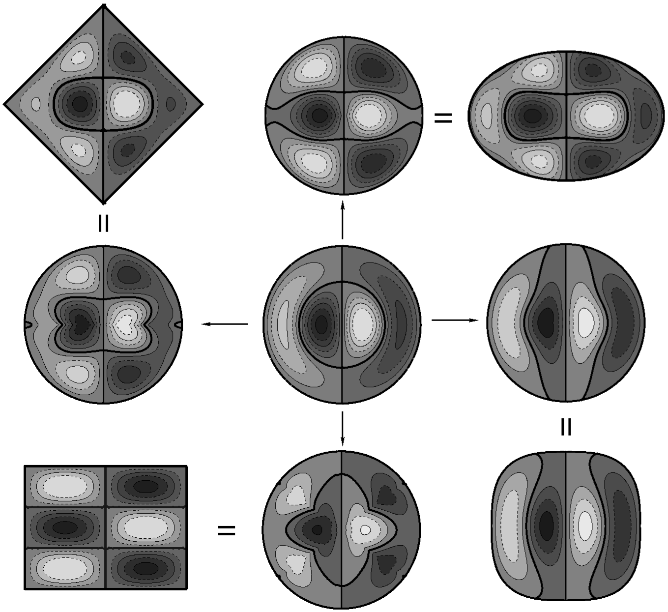
Figure 1: Contours (dashed and continuous black lines) and nodal lines (thick solid black lines) of the wavefunction for a particular case, say, $l=1$ and $j=2$. The figure in the center is that for a circular boundary of unit radius and is the starting point for all the four cases shown here. The figures pointed by the arrows in the right, left, up and down directions are the contours and nodal lines of the metric deformed wavefunction in a circular boundary and correspond to supercircular ($t=3$), square ($t=1$), elliptical ($\epsilon=0.75$, $a=1$) and rectangular (of length is to width ratio $4/3$) boundaries respectively. The figures next to these at corners are the plots of wavefunctions in their original shape.

The coefficient $a_{l}$ is calculated from the normalisation of the corrected wavefunction up to first order. These results are consistent with the ones obtained in earlier investigations [31, 32, 33]. The contours and the nodal lines of a wavefunction corrected up to first order for different boundary geometries are shown in Fig. 1. The small change in the nodal lines is visible for the case of supercircle deformation whereas for the other cases, viz. square, rectangle and ellipse, the changes are violent. At first glance it seems that one gets a wrong eigenmode for the square in the upper left corner of the Fig. 1. A closer look shows that it is indeed an eigenfunction of a square membrane where two degenerate modes, viz. (1,4) and (4,1), are mixed in equal proportion with a relative negative sign. Under deformation among the nodal lines only the line of symmetry is preserved as can be seen from the examples of Fig. 1. Moreover the number of crossings of the nodal lines is also not conserved for such violent perturbation. What seems to be preserved between the equivalent domains is the number of humps and valleys.

5 Results and Discussions

We next apply the analytical formalism developed in the earlier section to a few specific boundary geometries. We have compared our perturbative results against the numerical solutions obtained by using the Partial Differential Equation Toolbox^TM of MATLAB^®. To ensure the convergence of the eigenvalues in numerical method we have restricted only to convex domains. We have considered the case of a supercircle and an ellipse. The polar form for these two families of curves are respectively given by

$$r(\theta) =\frac{a}{(|\cos\theta|^{t}+|\sin\theta|^{t})^{1/t}}~{},$$ (21)

$$r(\theta) =\frac{a\sqrt{1-\epsilon^{2}}}{\sqrt{1-\epsilon^{2}\cos^{2}\theta}}~{}.$$ (22)

The parameters defining the boundaries are $(a>0,t\geq 1)$ and $(a>0,\epsilon>0)$ respectively. Eq. (21) defines a diamond ($45^{\circ}$ rotated square) for $t=1$, a circle for $t=2$, a supercircle for $t>1$ and $t\neq 2$ and a square as $t\rightarrow\infty$. The specific form of $r(\theta)$ for these closed curves are used to calculate the metric deformation and thereby estimate energy corrections. These curves are chosen because they have a reflection symmetry about y-axis and hence they can be represented by a Fourier series given in Eq. (4) with only cosine terms. The perturbative prescription is seen to converge with dominant non-zero corrections coming from the first few orders. It can be seen that the first and second order corrections in energy are linear and bi-linear in $C_{n}$ respectively. Further, it is clear that $E^{(m)}$ will be $m$-linear in $C_{n}$, hence convergence of the Fourier coefficients, $C_{n}$, will ensure the convergence of the series. In this analytic formalism the approximation appears only through truncation of the series given by Eqs. (7).

We have estimated energy corrections up to the second order in perturbation for the $l=0$ states and only first order corrections for the $l\neq 0$ states. The two-fold degeneracy of the original $l\neq 0$ states splits at the first order for $C_{2l}\neq 0$. In Figs. 2 and 3 we have illustrated the comparison of the analytical values calculated by our perturbation scheme with their respective numerical ones for the supercircular boundary in the range of $t$ from $1$ to $3$ for first few energy levels. Our results are in good agreement with the numerical ones. The discrepancy is $\sim 1\%$ for the supercircle within the range $1.5\leq t\leq 3$ and is relatively larger ($\sim 5\%$) as it tends toward the diamond shape, i.e., $t=1$. This larger discrepancy is anticipated because a square is a violent departure from a circle and this large deformation is against the inherent ingredient of the perturbative method. Furthermore, energy levels corresponding to some $l$ values exhibit level crossing phenomenon as reported earlier [32, 33]. It is clear from the Figs. 2 and 3 that the overall matching for the DBC is outstanding except for few occasions in case of square where only the first order correction (for $l\neq 0$ case) is included. However, inclusion of higher order corrections will definitely improve the accuracy of our method. In contrast, for the case of NBC most of the low-lying states with non-zero $l$ values do not even have the first order correction. So, in such cases the error is distinct for the square. The method is expected to yield better results for smooth boundaries without vertices. The results for the supercircle even at the first order show better accuracy than their second order counterparts for the square. Similarly, the comparison for elliptical boundaries is shown in Figs. 4 and 5. Here also, the agreement is highly satisfactory for a wide range of $\epsilon$ and the discrepancy is $\sim 2\%$. A typical comparison between the results obtained by numerical method ($Ns$) or the exact solution ($Es$) and our perturbative scheme ($Ps$) is shown in the Table 1.

In conclusion, we note that Fourier decomposition of the boundary asymmetry makes the method completely general and it holds good for a wide variety of boundaries and for general boundary conditions also. The main advantage of this method over the others is that it is boundary condition free and has general closed form solutions at every order of perturbation. Next it maintains the same simple form of boundary condition at every order of perturbation making the application of the boundary condition easier. In principle, the higher order corrections could also be calculated exactly but they are algebraically more complicated and tedious to evaluate. Since our solutions of the wavefunction are general (i.e. independent of boundary condition), the other mixed boundary conditions such as, Cauchy[35] or Robin[36], could also be applied to obtain the corresponding spectrum easily.

6 Acknowledgements

SP would like to acknowledge the Council of Scientific and Industrial Research (CSIR), India for providing the financial support. The authors would like to thank S. Bharadwaj, S. Kar, A. Dasgupta, S. Das and Ganesh T. for useful discussions and help. The authors would like to thank the referee for critical comments and suggestions for improving the text.

Figure 2: Comparison of the first few energy levels obtained numerically (denoted by points) and analytically (denoted by solid lines) for the supercircular boundary with the variation of the supercircular exponent ($t$) for fixed $a=1$ for DBC.

Figure 3: Comparison of the first few energy levels obtained numerically (denoted by points) and analytically (denoted by solid lines) for the supercircular boundary with the variation of the supercircular exponent ($t$) for fixed $a=1$ for NBC.

Figure 4: Comparison of the first few energy levels obtained numerically (denoted by points) and analytically (denoted by solid lines) for the elliptical boundary with the variation of the eccentricity ($\epsilon$) for fixed $a=1$ for DBC.

Figure 5: Comparison of the first few energy levels obtained numerically (denoted by points) and analytically (denoted by solid lines) for the elliptical boundary with the variation of the eccentricity ($\epsilon$) for fixed $a=1$ for NBC.

Table 1: Comparison of the first few energy eigenvalues with the magnitude of $\%$ error (= $\rvert\frac{Ns-Ps}{Ns}\lvert\times 100\%$ or $\rvert\frac{Es-Ps}{Es}\lvert\times 100\%$) for a supercircle (with $t=3,~{}a=1$), an ellipse (with $\epsilon=0.5,~{}a=1$) and a tilted square (with $t=1,~{}a=1$).

Supercircle			Ellipse			Square
$Ns$	$Ps$	$\%$	$Ns$	$Ps$	$\%$	$Es$	$Ps$	$\%$
		Error			Error			Error
Dirichlet Boundary Condition
5.219	5.217	0.04	6.744	6.744	0.00	9.870	10.129	2.62
13.193	13.076	0.89	15.893	15.776	0.74	24.674	23.317	5.49
13.202	13.076	0.95	18.339	18.218	0.66	24.674	23.317	5.49
22.372	22.141	1.03	29.080	30.416	4.59	39.478	36.047	8.69
25.088	24.838	1.00	30.725	30.652	0.24	49.348	47.726	3.29
27.157	27.138	0.07	37.191	37.777	1.58	49.348	49.533	0.37
36.042	36.254	0.59	45.762	47.115	2.96	64.152	64.648	0.77
36.046	36.254	0.58	46.570	47.136	1.22	64.152	64.648	0.77
44.449	43.835	1.38	54.937	52.886	3.73	83.892	78.166	6.82
44.490	43.835	1.47	62.334	61.073	2.03	83.892	78.166	6.82
50.967	51.203	0.46	65.343	66.662	2.02	88.826	87.429	1.57
Neumann Boundary Condition
2.975	3.019	1.48	3.426	3.407	0.55	4.935	5.384	9.09
2.978	3.019	1.38	4.462	4.442	0.45	4.935	5.384	9.09
7.136	7.115	0.29	10.387	10.695	2.97	9.870	9.648	2.25
9.524	9.500	0.25	10.846	10.904	0.53	19.739	19.981	1.23
12.788	12.779	0.07	17.563	17.596	0.19	19.739	20.059	1.62
15.513	15.719	1.33	20.067	20.419	1.75	24.674	28.031	13.61
15.529	15.719	1.22	20.206	20.448	1.19	24.674	28.031	13.61
25.100	25.039	0.24	31.018	30.370	2.09	39.478	37.785	4.29
25.190	25.315	0.50	32.288	32.733	1.38	44.413	45.141	1.64
25.232	25.315	0.33	32.322	32.736	1.28	44.413	45.141	1.64
25.246	25.327	0.32	35.969	35.442	1.47	49.348	52.028	5.43

References

- [1] J. W. S. B. Rayleigh, Theory of Sound : Vol 1 (Dover, New York, 1945).
- [2] P. M. Morse and H. Feshbach, Methods of Theoretical Physics: Vol 2 (McGraw Hill Book Company, 1953).
- [3] A. L. Fetter and J. D. Walecka, Theoretical Mechanics of Particles and Continua: Vol 2 (McGraw Hill Book Company, 1980).
- [4] I. Sobchenko, J. Pesicka, D. Baither, R. Reichelt and E. Nembachet, \JLAppl. Phys. Lett. ,89,2006,133107.
- [5] K. Lis, S. Bednarek, B. Szafran and J. Adamowski, \JLPhysica E,17,2003,494.
- [6] P. S. Drouvelis, P. Schmelcher and F. K. Diakonos, \PRB69,2004,155312.
- [7] I. Magnúsdóttir and V. Gudmundsson, \PRB60,1999,16591.
- [8] N. T. Gridgeman, \JLThe. Math. Gaz. ,54,1970,31.
- [9] L. Eyges, P. Gianino and P. Wintersteiner, \JLJ. Opt. Soc. Am. ,69,1979,1226.
- [10] R. Dubertrand, E. Bogomolny, N. Djellali, M. Lebental and C. Schmit, \PRA77,2008,013804.
- [11] B. A. Troesch and H. R. Troesch, \JLMath. Comput. ,27,1973,755.
- [12] R. C. T. George and P. R. Shaw, \JLJ. Acoust. Soc. Am. ,56,1974,796.
- [13] J. Mazumdar, \JLShock Vib. Dig. ,14,1982,11.
- [14] J. R. Kuttler and V. G. Sigillito, \JLSIAM Review,26,1984,163.
- [15] M. Robnik, \JLJ. Phys. A: Math. Gen. ,17,1984,1049.
- [16] R. Hettich, E. Haaren, M. Ries and G. Still, \JLJ. Appl. Math. Mech. ,67,1987,589.
- [17] D. L. Kaufman, I. Kosztin and K. Schulten, \JLAm. J. Phys. ,67,1999,133.
- [18] D. Cohen, N. Lepore and E. J. Heller, \JLJ. Phys. A: Math. Theor. ,37,2004,2139.
- [19] A. H. Barnett and T. Betcke, \JLCHAOS, 17,2007,043125.
- [20] H. B. Wilson and R. W. Scharstein, \JLJ. Eng. Math. ,57,2007,41.
- [21] P. Amore, \JLJ. Phys. A: Math. Theor. ,41,2008,265206.
- [22] P. Guidotti and J. Lambers, \JLNumer. Func. Anal. Opt. ,29,2008,507.
- [23] E. Lijnen, L. F. Chibotaru and A. Ceulemans, \PRE77,2008,016702.
- [24] P. Amore, \JMP51,2010,052105.
- [25] A. H. Nayfeh, Introduction to Perturbation Techniques: Vol 1 (J. Wiley, New York, 1981).
- [26] J. K. Bhattacharjee and K. Banerjee, \JLJ. Phys. A: Math. Gen. ,20,1987,L759.
- [27] W. W. Read, \JLMath. Comput. Model. ,24,1996,23.
- [28] L. Molinari, \JLJ. Phys. A: Math. Gen. ,30,1997,6517.
- [29] Y. Wu and P. N. Shivakumar, \JLComput. Math. Appl. ,55,2008,1129.
- [30] N. Bera, J. K. Bhattacharjee, S. Mitra and S. P. Khastgir, \JLEur. Phys. J. D,46,2008,41.
- [31] R. G. Parker and C. D. Jr. Mote, \JLJ. Sound and Vib. ,211,1998,389.
- [32] S. Chakraborty, J. K. Bhattacharjee and S. P. Khastgir, \JLJ. Phys. A: Math. Gen. ,42,2009,195301.
- [33] S. Panda, S. Chakraborty and S. P. Khastgir, \JLEur. Phys. J. Plus,126,2011,62.
- [34] E. Schrödinger, \JLAnn. Physik,80,1926,437.
- [35] L. Marin, L. Elliott, P. J. Heggs, D. B. Ingham, D. Lesnic and X. Wen, \JLComput. Mech. ,31,2003,367
- [36] B. J. McCartin, \JLInternat. J. Math. Math. Sci. ,2004,2004,807.