2D massless QED Hall half-integer conductivity and graphene

Abstract

Starting from the photon self-energy tensor in a magnetized medium, the 3D complete antisymmetric form of the conductivity tensor is found in the static limit of a fermion system $C$ non-invariant under fermion-antifermion exchange. The massless relativistic 2D fermion limit in QED is derived by using the compactification along the dimension parallel to the magnetic field. In the static limit and at zero temperature the main features of quantum Hall effect (QHE) are obtained: the half-integer QHE and the minimum value proportional to $e^{2}/h$ for the Hall conductivity . For typical values of graphene the plateaus of the Hall conductivity are also reproduced.

1 Introduction

In 2004, graphene - genuine monolayer of carbon atoms in a honeycomb array - was obtained experimentally [1, 2]. The theoretical description of this material was studied with some anticipation [3]-[4] to the experimental results [5]-[7] and the analogy to the 2D quantum electrodynamics and some particular features of this system were examined in the 1980s [8]-[10]. The experimental confirmation of its existence obtained as isolated individual graphene layers leads to increase the theoretical and experimental studies of its properties with the aim to look for nanoescale electronic applications.

Theoretically, its properties are essentially described by Dirac massless fermions (electrons) in two dimensions. This system is relativistic in the sense that the spectra of electrons and holes can be mimicked as two-dimensional relativistic chiral fermions where electrons and holes move at velocities $v_{F}\approx 10^{6}m/s$ one hundredth the speed of light [11].

Being the quasiparticles chiral charged massless Dirac fermions, this has triggered a lot of papers from physicists from high energy physics (for exhaustive review see Ref. [12] and references therein). From the point of view of high energy physics graphene could be interesting to test some quantum field theories and their features in the well known QED, in table top experiments [13] and provides the possibility to explore exotic phenomena which could be important for cosmology and astrophysics [14]-[15].

Emerging from theoretical studies of graphene by methods and technics from Quantum Field Theory (QFT) and condensed matter physics, one of the main challenges is to gain understanding and matching between both descriptions and interpretations.

On the other hand the boom in the applications demand the study of transport properties [16], [17], such as conductivity [18]-[20] and QHE [21]-[29], theoretically as well as experimentally [30]-[38].

The most remarkable result related to the graphene Hall conductivity is the typical plateau structure for integer quantum filling factors and the non-zero value of the Hall conductivity when the carrier density goes to zero [11] and these properties have been related to the relativistic nature of the graphene dynamics [32]-[37].

The effect has been observed for densities around $10^{12}cm^{-2}$, magnetic fields strength in the range of $15-25T$ even at room temperature.

Inspired by these results of QH of graphene we have as a main goal of the present paper to revisit the relativistic QHE, especially the 2D case. Our starting point will be the conductivity tensor derived in the static limit from the quantum relativistic electron self-energy tensor in QED in presence of a magnetic field.

As different to [41] in which 3D and 2D QHE was studied with the motivation to apply the results to condensed matter physics, in the present paper we consider it as model for graphene-like systems. We start from the simple model of a charged fermion-antifermion plasma in a magnetic field which is also interacting perturbatively with an electromagnetic wave. The study was done by using the methods of finite temperature quantum field theory in the search of its kinetic properties. Two properties are found for the conductivity tensor. First, in the static limit, $\omega=0$, $k=0$, it is found that the conductivity tensor is given by a complete antisymmetric expression for the 3D as well as 2D cases. Second, the Hall conductivity as a function of the external magnetic field in the 2D case exhibits the typical plateaus structure of the integer QHE at zero temperature limit under the hypothesis of variable number of particles [42]-[43]. The formalism is a general method, also valid for studying the cases $\omega\neq 0$, and $k\neq 0$.

The outcomes of the present paper are interesting due to several facts: first, we find the conductivity tensor for both the 3D and 2D cases, by starting from a massive system, for which we get the massless limit. (The 2D is obtained as a compactification of the 3D case, since we are interested in the Hall conductivity of a graphene-like system). Second, our general expressions can be used for studying the static as well as the non-static limits. Third, the non-vanishing of the conductivity in the lowest Landau level occupancy (leading to the magnetic catalysis) is a consequence of the $C$-non-invariance of the system. We must also mention that our basic equations may be used also for studying wave propagation phenomena, such as Faraday effect; this, however, is out of the scope of the present paper.

Our results are valid at the one-loop level, for magnetic fields not very high ($B<<20$ T). Experimental results [44],[45] suggest that higher magnetic fields would demand to introduce higher loops.

The paper is organized as follows. In section 2 we briefly recall the expression for the charged fermions Green function in a constant magnetic field [39], in section 3 is obtained the current density and Hall conductivity starting from the photon self-energy. In Section 4 the QH conductivity is found for the 2D massless fermion system using the compactification of z-dimension. Finally it is shown the QHE for the graphene-like system. The conclusions are drawn in section 5.

2 Green functions for charged fermions in presence of a magnetic field

In this section we outline how to obtain the one particle Green function in a medium, e.g., for a system of charged fermions in presence of the constant magnetic field at finite temperature $T=1/\beta$ and density characterized by a chemical potential $\mu$. It is necessary for the calculation of the photon self-energy tensor from which the conductivity tensor will be found. In this section we will take $m\neq 0$ in our expressions and in the next Section we will take the limit $m=0$.

The temperature dependent Green function for a gas of charged and fermions and anti-fermions in a constant external magnetic field (which we will take parallel to the third axis) $A_{\nu}=Bx_{1}\delta_{2\nu}$, is given by the solution of the Dirac equation

$$[\gamma_{\nu}(\partial_{\nu}+ieA_{\nu})+m]G(x,x^{\prime}|A)=\delta(x-x^{\prime}),$$ (1)

where $\nu=1,2,3,4$, $\partial_{4}=\partial/\partial_{4}-\mu$, and $\mu$ is the chemical potential of the system. The temperature Green functions are determined by (1) for $-\beta<x_{4}<\beta$, where $\beta=\frac{1}{kT}$, $k$ is the Boltzmann constant. For simplicity we use $k=\hbar=c$ and recover the units at the end of the paper.

According to the established procedure, to obtain the solution of (1) we start from the Fourier transform in time of the time dependent Green function, the Fourier parameter $p_{0}$ is then continued to the complex value $-ip_{4}+\mu$, and the resulting expression, multiplied by $e^{ix_{4}p_{4}}$, is summed over the Matsubara frequencies $p_{4}=\frac{(2s+1)\pi}{\beta}$, and $s$ runs from $-\infty$ to $-\infty$. The time dependent Green function can be built from the solutions of the Dirac equation in relativistic quantum mechanics. We use the following energy eigenfunctions, according to [47]-[48], the signs $\pm$ correspond to positive and negative energy solutions, respectively

$$\phi^{\pm}_{p_{2},p_{3},n,1}(\mathbf{x}) = \large(\frac{\varepsilon_{n,p_{3}}\pm m}{8\pi^{2}\varepsilon_{n,p_{3}}}\large)^{1/2}e^{ip_{2}x_{2}+ip_{3}x_{3}}\left(\begin{array}[]{c}\psi_{n-1}(\xi)\\ 0\\ \frac{\pm p_{3}}{(\varepsilon_{n,p_{3}}\pm m)}\psi_{n-1}(\xi)\\ \frac{\pm i(2eBn)^{1/2}}{(\varepsilon_{n,p_{3}}\pm m)}\psi_{n}(\xi)\\ \end{array}\right),$$ (6)

$$\phi^{\pm}_{p_{2},p_{3},n,-1}(\mathbf{x}) = \large(\frac{\varepsilon_{n,p_{3}}\pm m}{8\pi^{2}\varepsilon_{n,p_{3}}}\large)^{1/2}e^{ip_{2}x_{2}+ip_{3}x_{3}}\left(\begin{array}[]{c}0\\ \psi_{n}(\xi)\\ \frac{\mp i(2eBn)^{1/2}}{(\varepsilon_{n,p_{3}}\pm m)}\psi_{n-1}(\xi)\\ \frac{\mp p_{3}}{(\varepsilon_{n,p_{3}}\pm m)}\psi_{n}(\xi)\\ \end{array}\right).$$ (11)

Here the subindex $(p_{2},p_{3},n,\sigma)$ refers to the $p_{2},p_{3}$ momenta, to the total quantum number $n$ and to the spin $\sigma_{3}$-eigenvalues $\sigma_{3}=\pm 1$, respectively. The energy eigenvalues are

$$\varepsilon_{n,p_{3}}=\sqrt{p_{3}^{2}+m^{2}+2neB}.$$ (12)

These are two fold spin degenerate, except for $n=0,\sigma_{3}=-1$, and are also $p_{2}$ degenerate.

We have written $\xi=\sqrt{eB}(x_{1}+x_{0}),$ with $x_{0}=p_{2}/eB$ being the eigenvalue of the $x_{1}$ coordinate operator of the center of the orbit described by the particle) and

$$\psi_{n}(\xi)=\frac{(eB)^{1/4}}{\pi^{1/4}2^{n/2}(n!)^{1/2}}e^{-\frac{\xi^{2}}{2}}H_{n}(\xi),$$ (13)

are the Hermite functions multiplied by $(eB)^{1/4}$.

The time dependent Green function in the Furry picture is

$$G(\mathbf{x},t,\mathbf{x^{\prime}},t^{\prime})=\left\{\begin{array}[]{cccc}-i\displaystyle\sum\limits_{q}e^{-i\varepsilon_{q}(t-t^{\prime})}{\cal{G}}_{q}^{+}(\mathbf{x},\mathbf{x^{\prime}})&&\textrm{for}&t>t^{\prime}\\ \\ i\displaystyle\sum\limits_{q}e^{i\varepsilon_{q}(t-t^{\prime})}{\cal{G}}_{q}^{-}(\mathbf{x},\mathbf{x^{\prime}})&&\textrm{for}&t<t^{\prime}\\ \end{array}\right.\hskip 14.22636pt,$$ (14)

where $q$ denotes the set of quantum numbers $(p_{2},p_{3},n)$, $\displaystyle\sum\limits_{q}$ indicates integration on $p_{2},p_{3}$ and sum over $n=0,1,2,...$ and (the bar means Dirac adjoint). Here

$${\cal{G}}_{q}^{\pm}(\mathbf{x},\mathbf{x^{\prime}}) = \sum_{\sigma}\phi^{\pm}_{q,\sigma}(\mathbf{x})\bar{\phi}^{\pm}_{q,\sigma}(\mathbf{x^{\prime}})$$ (15)

$$= \frac{e^{ip_{2}(x_{2}-x^{\prime}_{2})+ip_{3}(x_{3}-x^{\prime}_{3})}}{8\pi^{2}\varepsilon_{n,p_{3}}}\Lambda_{q},$$

where

$$\Lambda_{q}=\left(\begin{array}[]{cccc}C_{n-1,n-1}(\varepsilon_{n,p_{3}})&0&-D_{n-1,n-1}&-E_{n-1,n}\\ 0&C_{n,n}(\varepsilon_{n,p_{3}})&E_{n,n-1}&D_{n,n}\\ D_{n-1,n-1}&E_{n-1,n}&C_{n-1,n-1}(-\varepsilon_{n,p_{3}})&0\\ -E_{n,n-1}&-D_{n,n}&0&C_{n,n}(-\varepsilon_{n,p_{3}})\\ \end{array}\right),$$

and

$$C_{k,k^{\prime}}(\varepsilon_{n,p_{3}})=(\varepsilon_{n,p_{3}}\pm m)\psi_{k}(\xi)\psi_{k^{\prime}}(\xi^{\prime}),\hskip 14.22636ptD_{k,k^{\prime}}=\pm p_{3}\psi_{k}(\xi)\psi_{k^{\prime}}(\xi^{\prime}),$$

$$E_{k,k^{\prime}}=\mp i(2eBn)^{1/2}\psi_{k}(\xi)\psi_{k^{\prime}}(\xi^{\prime}).$$

It is understood in (14) that $\psi_{-1}(\xi)\equiv 0$. Taking the Fourier transform in time of (14), and making the continuation $p_{0}\rightarrow-ip_{4}+\mu$, we get for the $x_{4}$ Fourier transform of the solution of (1)

$$G(-ip_{4}+\mu,\mathbf{x},\mathbf{x^{\prime}})=\frac{{\cal{G}}_{q}^{+}(\mathbf{x},\mathbf{x^{\prime}})}{-ip_{4}+\mu-\varepsilon_{n,p_{3}}}+\frac{{\cal{G}}_{q}^{-}(\mathbf{x},\mathbf{x^{\prime}})}{-ip_{4}+\mu+\varepsilon_{n,p_{3}}}.$$ (16)

After multiplication by $e^{ip_{4}x_{4}}$ and summation over $p_{4}$ we have the following expression for the temperature dependent Green function:

$$G(\mathbf{x},\mathbf{x^{\prime}}) = \displaystyle\sum_{q}\left[(n_{e}(\varepsilon_{n,p_{3}})-1)e^{-(\varepsilon_{n,p_{3}}-\mu)(x_{4}-x^{\prime}_{4})}{\cal{G}}_{q}^{+}(\mathbf{x},\mathbf{x^{\prime}})\right.$$

$$\hskip 59.75095pt\left.-n_{p}(\varepsilon_{n,p_{3}})e^{(\varepsilon_{n,p_{3}}+\mu)(x_{4}-x^{\prime}_{4})}{\cal{G}}_{q}^{-}(\mathbf{x},\mathbf{x^{\prime}})\right]\hskip 5.69046pt\textrm{for }x_{4}>x^{\prime}_{4},$$

$$G(\mathbf{x},\mathbf{x^{\prime}}) = \displaystyle\sum_{q}\left[n_{e}(\varepsilon_{n,p_{3}})e^{-(\varepsilon_{n,p_{3}}-\mu)(x_{4}-x^{\prime}_{4})}{\cal{G}}_{q}^{+}(\mathbf{x},\mathbf{x^{\prime}})\right.$$

$$\hskip 28.45274pt\left.-(n_{p}(\varepsilon_{n,p_{3}})-1)e^{(\varepsilon_{n,p_{3}}+\mu)(x_{4}-x^{\prime}_{4})}{\cal{G}}_{q}^{-}(\mathbf{x},\mathbf{x^{\prime}})\right]\hskip 5.69046pt\textrm{for }x_{4}<x^{\prime}_{4},$$

where

$$n_{e}(\varepsilon_{n,p_{3}}) = \frac{1}{1+e^{(\varepsilon_{n,p_{3}}-\mu)\beta}},$$

$$n_{p}(\varepsilon_{n,p_{3}}) = \frac{1}{1+e^{(\varepsilon_{n,p_{3}}+\mu)\beta}},$$ (18)

are the mean number of fermions and anti-fermions, respectively.

Later we will be interested in the massless and 2D limits of the Green function (2).

3 Current density and conductivity from the photon self-energy

This section is devoted to obtain the general expression of the conductivity tensor for the quantum relativistic fermion plasma which is linear in the perturbative electromagnetic field $A_{\mu}$. In Euclidean variables we have the Maxwell equations $D_{0\mu\nu}^{-1}A_{\nu}=j_{\mu}(A)$, where $D_{0\mu\nu}^{-1}=(\partial_{\lambda}^{2}\delta_{\mu\nu}-\partial_{\mu}\partial_{\nu})$

Our starting point will be the linear term in $A_{\mu}$ in the expansion of $j_{\mu}(A)$ in powers of $A_{\lambda}$, the coefficient being the photon self-energy tensor. The current density can be written as

$$j_{i}=\pi_{i\nu}A_{\nu}=Y_{ij}E_{j},\,\,\,\nu=1,2,3,4,\,\,\,i=1,2,3,$$ (19)

where $E_{j}=i(\omega A_{j}-k_{j}A_{0})$ is the electric field of the electromagnetic wave, $A_{4}=iA_{0}$, $k_{4}=i\omega$ and $Y_{i,j}=\pi_{ij}/i\omega$ is the complex conductivity tensor or admittivity, and the third term in (19) comes from the second one by using the four-dimensional transversality of $\pi_{\mu\nu}$, $\pi_{\mu\nu}k_{\nu}=0$, due to gauge invariance.

We are interested in the real conductivity which can be expressed in terms of the imaginary part of the photon self-energy and the frequency as $\sigma_{ij}=\mathrm{Im}\pi_{ij}/\omega$ [39].

The components of the photon self-energy tensor in the case of non zero temperature and density and in presence of the external magnetic field $B$ can be obtained from

$$\pi_{\nu\mu}(x,y)=e^{2}Tr\int\gamma_{\mu}G(x,z)\Gamma_{\nu}(z,y^{\prime},y)G(y^{\prime},x)d^{3}zd^{3}y^{\prime}.$$ (20)

$G(y^{\prime},x)$ is the Green function of the charged fermions obtained in section I and $\Gamma_{\nu}$ is the vertex function which in one loop approximation has the form $\Gamma_{\nu}=\gamma_{\nu}\delta(z-y^{\prime})\delta(z-y)$.

In [39]-[40] it was obtained the expression (20) for electron positron plasma. Details of the calculations can be seen there. In that paper it was shown that $\pi_{\mu\nu}$ can be expressed as a linear combination of the six four-dimensional transverse tensors, four of them symmetric and two antisymmetric with respect to the indices $\mu,\nu$, $\pi_{\mu\nu}=\sum_{i=1}^{6}\pi^{i}\Phi^{i}_{\mu\nu}$. The scalar coefficients $\pi^{(i)}$ in that expansion are expressed in terms of six scalars functions $p,t,s,q,r$ and $v$ [39](after the dimensional reduction $3+1\to 2+1$ the scalars $q$ and $v$ vanish and the number of independent scalars is reduced to four, $p,t,s,r$). By studying the analytic properties of $\pi_{\mu\nu}$ it was proved that the imaginary components of its symmetric part are due to the singularities produced by the photon absorptive processes (excitations of the electrons and positrons and pair creation), whereas the imaginary part of its antisymmetric terms is connected with the interaction of the net charge and current of the electron-positron system with the external magnetic field. The first mechanism contributes to Ohm conductivity whereas the second, to Hall conductivity.

Let us note that all these arguments can be extended to our present calculation and the contribution to the current density $j_{i}$ in the equation (19) due to conductivity can be written then in the general form as

$$j_{i}=\sigma_{ij}^{0}E_{j}+(E\times\mathcal{S})_{i},$$ (21)

where $\sigma_{ij}^{0}=\mathrm{Im}\pi_{ij}^{S}/\omega$ and $\mathcal{S}_{i}=\frac{1}{2}\epsilon^{ijk}\sigma_{jk}^{H}$ is a pseudovector associated to $\sigma_{jk}^{H}=\mathrm{Im}\pi_{ij}^{A}/\omega$, $\pi_{ij}^{S}$, $\pi_{ij}^{A}$ are the symmetric and antisymmetric parts of the spatial photon self-energy. The first term in (21) corresponds to the Ohm current and the second is the Hall current E is the electric field corresponding to the electromagnetic wave eigenmodes of $\pi_{\mu\nu}$. Let us consider the specific case when the electric field $\mathbf{E}$ is due to a transverse mode propagating along the magnetic field $\mathbf{B}$, and thus $\mathbf{E}$ is perpendicular to $\mathbf{B}$ and does not depend on the components $k_{1},k_{2}$ $(\mathbf{B}\parallel k_{3})$. The expression for the conductivity, according to [41], is

$$\sigma_{ij}=\sigma^{0}_{3D}\delta_{ij}+\epsilon^{ij}\sigma^{H}_{3D},$$ (22)

where $\epsilon^{ij}$ is the antisymmetric $2\times 2$ unit tensor, $\epsilon^{12}=-\epsilon^{21}=1$ and $\sigma^{0}_{3D}=\mathrm{Im}t/\omega$, $\sigma^{H}_{3D}=\mathrm{Im}r/\omega$ and the expressions for the scalar quantities $\mathrm{Im}t$, $\mathrm{Im}r$ were found in [41]. Let us take the limit $m\to 0$, that is, let us consider a version of QED in the fermion massless limit. This would require a more detailed discussion, since chiral invariance appears and also the Feynman diagrams and renormalizability must be discussed in the new context. We assume that limit as satisfactory and proceed with its consequences. We have now

$$\mathrm{Im}t=\frac{e^{3}B}{4\pi}\sum\limits_{n,n^{\prime}=0}^{\infty}\frac{\Upsilon(\delta_{n,n^{\prime}-1}+\delta_{n-1,n^{\prime}})[N^{+}(\epsilon_{q})-N^{+}(\epsilon_{q}+\omega)]}{\sqrt{(z_{1}+2eB(n-n^{\prime}))^{2}+4z_{1}\varepsilon_{n,0}}},$$ (23)

where

$$\Upsilon=z_{1}+2eB(n+n^{\prime}),\hskip 14.22636ptz_{1}=(k_{3}^{2}-\omega^{2}),\hskip 14.22636ptN^{+}(\epsilon_{q})=n_{e}(\epsilon_{q})+n_{p}(\epsilon_{q}),\hskip 14.22636pt$$

$$\epsilon_{q}=\frac{-\omega z_{1}+|k_{3}|\sqrt{(z_{1}+2eB(n-n^{\prime}))^{2}+4z_{1}\varepsilon_{n,0}}}{2z_{1}},\,\,\,\varepsilon_{n,0}=\sqrt{2eBn}$$

and

$$\mathrm{Im}r=\frac{e^{3}B\omega}{2\pi}\sum\limits_{n,n^{\prime}=0}^{\infty}(\delta_{n,n^{\prime}-1}-\delta_{n-1,n^{\prime}})\int dp_{3}\frac{\Upsilon}{|Q|^{2}}(n_{e}(\varepsilon_{n,p_{3}})-n_{p}(\varepsilon_{n,p_{3}})),$$ (24)

$$|Q|^{2}=[2p_{3}k_{3}-z_{1}+2eB(n-n^{\prime})]^{2}-4\omega^{2}(2eBn).$$

It is easy to prove that in the static limit $\omega=0$, $k_{3}=0$, the conductivity tensor becomes completely antisymmetric ($\sigma^{0}_{3D}=0$), because the term $\mathrm{Im}t/\omega$ vanishes in that limit [41] and the conductivity is $\sigma_{ij}=\sigma^{H}_{3D}\epsilon^{ij}$. However, the Hall conductivity is non zero in the same limit and it has the form

$$\sigma^{H}_{3D}=\frac{e^{2}}{4\pi^{2}}\sum_{n=0}^{\infty}\alpha_{n}\int_{-\infty}^{\infty}dp_{3}(n_{e}(\varepsilon_{n,p_{3}})-n_{p}(\varepsilon_{n,p_{3}})),\hskip 28.45274pt\alpha_{n}=2-\delta_{0n}.$$ (25)

The expression (25) is valid for the massive as well as for the massless limit. If the system is $C$-invariant, as in a neutral gas of electrons and positrons, $\mu=0$ and it implies $\sigma^{H}_{3D}=0$. No Hall current is excited. But if the system is not $C$-invariant, as it happens in ordinary matter composed from charged baryons and leptons, this is not the case (see below). At zero temperature and for $\mu>0$ ($\mu<0$) the contribution of antifermions (fermions) is zero, the fermion gas is completely degenerate, and $\sigma^{H}_{3D}$ takes in the massless case the form

$$\sigma^{H} = \pm\frac{e^{2}}{4\pi^{2}}\sum_{n=0}^{n_{\mu}}\alpha_{n}\int\limits_{-\infty}^{\infty}dp_{3}\theta(\mu\mp\varepsilon_{n,p_{3}})$$ (26)

$$= \pm\frac{e^{2}}{4\pi^{2}}\sum_{n=0}^{n_{\mu}}\alpha_{n}\sqrt{\mu^{2}-2eBn}.$$

where $n_{\mu}=I(\mu^{2}/2eB)$, and $\theta(x)$, $I(x)$ are the step and the integer functions, respectively. Obviously, for $\mu<\sqrt{2eB}$ only the lowest Landau level (LLL) is occupied and $\sigma^{H}=\pm\frac{e^{2}}{4\pi^{2}}\mu$ does not depend explicitly on $B$. However, if the density $N$ is fixed, $\mu$ depends both on $N$ and on $B$ . But if $\mu$ is fixed, the condition of occupying only the LLL is always achieved by choosing $B$ large enough. Actually, this is valid even in the massive case, as is seen if in the previous inequality $\mu$ is replaced by $\mu^{\prime}=\sqrt{\mu^{2}-m^{2}c^{4}}$ as the effective chemical potential.

We must emphasize that the properties of (25)-(26) come from the scalar $r$ which as well as other components of $\pi_{\mu\nu}$ emerge from the relativistic, charge conjugation, parity and time reversal CPT and gauge invariance of QED.

Our next step will be to obtain the relativistic 2D Hall conductivity which describe a graphene-like system.

4 2D massless fermion conductivity

Let us describe the 2D massless QED behavior as an effective 2D theory, which is obtained from the 3D one, after dimensional compactification. To that end we assume that the coordinate $z$ is compact with a certain compactification length $L_{3}$; that is, $z$ varies in the interval $0\leq z\leq L_{3}$, and points $z=0$ and $z=L_{3}$ are identified. The momentum along the $z$ direction will be then quantized $p_{3}=2\pi s/L_{3}$, $s=0,1,2,...$, and below the energy scale $E_{0}=2\pi/L_{3}$ only zero modes with $s=0$ (corresponding to $p_{3}=0$) are relevant, i.e. the theory is effectively two-dimensional. In this reduced space, the external magnetic field $B$ behaves like a pseudo-scalar. In this section we will return to units $c$, $h=2\pi\hbar$, starting from equation (39).

The mentioned zero modes with $p_{3}=0$ satisfy then the reduced Dirac equation

$$\gamma_{\nu}(\partial_{\nu}+ieA_{\nu})G(x,x^{\prime}|A)=\delta(x-x^{\prime}),$$ (27)

where $\nu=1,2,4$, and the corresponding energy eigenfunctions are the $m=0$, $p_{3}=0$ limits of (6)

$$\phi^{\pm}_{p_{2},0,n,1}(\mathbf{x}) = \frac{1}{2\pi^{1/2}L_{3}}e^{ip_{2}x_{2}}\left(\begin{array}[]{c}\psi_{n-1}(\xi)\\ 0\\ 0\\ \pm i(2eBn)^{1/2}\varepsilon_{n,0}^{-1}\psi_{n}(\xi)\\ \end{array}\right),$$ (32)

$$\phi^{\pm}_{p_{2},0,n,-1}(\mathbf{x}) = \frac{1}{2\pi^{1/2}L_{3}}e^{ip_{2}x_{2}}\left(\begin{array}[]{c}0\\ \psi_{n}(\xi)\\ \mp i(2eBn)^{1/2}\varepsilon_{n,0}^{-1}\psi_{n-1}(\xi)\\ 0\\ \end{array}\right).$$ (37)

The eigenvalues $\sigma_{3}=\pm 1$ are now interpreted, from the 2D point of view, as the pseudo spin quantum numbers, and the energy eigenvalues are simply

$$\varepsilon_{n,0}=\sqrt{2neB}.$$ (38)

Let us remark that as different from the $3+1$ QED in which there is only one $4\times 4$ irreducible representation for the Dirac $\gamma$-matrices, in $2+1$ dimensions [49] there are two $2\times 2$ inequivalent irreducible representations of $\gamma$-matrices (which in graphene correspond to two points of the Fermi surface, $K$ and $K^{\prime}$ describing respectively states on sublattices ($A$ , $B$) of the hexagonal lattice). Therefore, the dimensional reduction we have made correspond to the sum of these two $2\times 2$ irreducible representations. However, from (37), which is the $2D+1$ limit of (6), we see that to each spin state $\pm 1$ correspond two (obviously inequivalent) positive and negative energy eigenstates $\phi^{\pm}$.

All the expressions obtained previously from the photon self-energy are translated immediately to the 2D case. For instance, in the static limit $\omega=0$ ($k_{3}=0$ by assumption), and to obtain the zero mode 3D Hall conductivity we should substitute in (24) $p_{3}=2\pi s/L_{3}$, replace the integral over $p_{3}$ by a sum over the integers $s$ and retain only the $s=0$ term. Then, the corresponding zero mode 2D Hall conductivity $\sigma^{H}_{2D}\equiv L_{3}\sigma^{H}_{3D}$ is

$$\sigma^{H}_{2D} = \frac{L_{3}\mathrm{Im}r}{\omega}$$ (39)

$$= \frac{e^{2}}{h}\sum_{n=0}^{\infty}\alpha_{n}(n_{e}(\varepsilon_{n,0})-n_{p}(\varepsilon_{n,0})).$$

At zero temperature, for positive (negative) chemical potential $\mu>0$ ($\mu<0$), the contribution of antifermions (fermions) is zero, the fermion (antifermion) gas is completely degenerate. Taking into account the spectrum energy (38) and by considering that the chemical potential is $n_{\mu}<|\mu^{2}|/2eB<n_{\mu}+1$, we obtain for $\sigma^{H}_{2D}$

$$\sigma^{H}_{2D}=\left\{\begin{array}[]{cccc}\displaystyle\frac{e^{2}}{h}\sum\limits_{n=0}^{n_{\mu}}\alpha_{n}\theta(\mu-\varepsilon_{n,0})=2\frac{e^{2}}{h}\left(n_{\mu}+\frac{1}{2}\right)&&\textrm{for}&\mu>0\\ \\ -\displaystyle\frac{e^{2}}{h}\sum\limits_{n=0}^{n_{\mu}}\alpha_{n}\theta(\mu+\varepsilon_{n,0})=-2\frac{e^{2}}{h}\left(n_{\mu}+\frac{1}{2}\right)&&\textrm{for}&\mu<0\\ \end{array}\right.\hskip 14.22636pt.$$ (40)

The expression (40) describes the anomalous Hall conductivity of the 2D relativistic massless fermions and antifermions.

4.1 Thermodynamical potential for 2D fermions

The Hall conductivity obtained before can be derived from the 2D thermodynamical potential which is obtained from the 3D expression [46] and has the following form

$$\Omega_{2D}=-\frac{eB}{hc\beta}\sum_{n=0}^{\infty}\alpha_{n}\ln(1+e^{-(\varepsilon_{n,0}-\mu)\beta})(1+e^{-(\varepsilon_{n,0}+\mu)\beta}).$$ (41)

The particle density is $N=-\frac{\partial\Omega}{\partial\mu}$, for the 2D system at zero temperature has the form

$$N_{2D}=\frac{eB}{hc}\sum_{n=0}^{\infty}\alpha_{n}\theta(\mu-\varepsilon_{n,0}).$$ (42)

The expression for the density (42) shows a non-zero value at the LLL. This leads to the so-called magnetic catalysis (MC) phenomenon, a chiral symmetry breaking determined by the dimensional reduction of the charged system in a magnetized medium [28]. Consequently the absolute value of the 2D Hall conductivity (40) has a minimum value of order $2\frac{e^{2}}{h}$ for small $\mu>T\to 0$ such that $0<\frac{\mu^{2}}{2eB}<1$.

In presence of an uniform electric field it has been proved in [25] that the minimum quantum conductivity in graphene is $4e^{2}/h$.

It is possible to rewrite the Hall conductivity (40) in terms of the particle density as given by the well-known classical expression [50] as

$$\sigma^{H}_{2D}=\frac{ecN_{2D}}{B},$$ (43)

which is a result obtained for 3D Hall conductivity but we take now $N$ as the 2D density, (number of particles per unit area).

This result agree with the calculations presented in [21] where the authors have started from the effective action of the 2D fermion gas in presence of a magnetic field which is equivalent to the treatment of the thermodynamical potential as a way to confirm that our results, obtained through the photon self energy, are in agreement with the more usual form of dealing with the Hall conductivity.

Previously we have dealt with a C-invariant system of particles-antiparticles (as electrons and positrons) being their chemical potentials $\mu_{e}=\mu$, $\mu_{p}=-\mu$ in the frame of QED at finite temperature. As we want to understand our results as a graphene-like system, we note that for graphene the electron-hole subsystem behaves also as C-invariant [51]. Thus, we must replace the positron distribution $n_{p}$ by the hole distribution $n_{h}$ in (39)). We get then at $T\neq 0$, that if $\mu=0$, the carrier density $N_{e,h}=\frac{eB}{hc}\sum_{n=0}^{\infty}\alpha_{n}(n_{e}-n_{h})=0$ and in consequence $\sigma^{H}_{2D}=0$, the Hall conductivity goes smoothly to zero when the chemical potential swaps from negative to positive values [18].

4.2 Graphene half-integer Hall conductivity

Expressions (40), (43) can also describe a graphene like half-integer Hall conductivity by substituting for the values of the typical parameters of graphene. In addition to the the spin degeneracy, an extra factor two comes from the sublattice-valley degeneracy in graphene. Also the substitution $c\rightarrow v_{F}^{2}/c$, where $v_{F}$ is the Fermi velocity must be made in the energy eigenvalue equation and in other corresponding places). Finally we get the well known expression for the graphene Hall conductivity (measured in c.g.s. units) as

$$\sigma^{H}=\pm 4\frac{e^{2}}{h}(n_{g}+1/2),\hskip 28.45274ptn_{g}=I(\frac{\mu^{2}c}{2eB\hbar v_{F}^{2}}).$$ (44)

In Figs. 1 and 2 we have plotted the Hall conductivity as a function of magnetic field and density for typical values of the experiments where QHE has been observed. As can be seen, the degenerate limit ($T=0$) describes quite well the behavior for $T\ll T_{F}$ which, is fulfilled for graphene-like system where the effect is observed at room temperatures (300 K) with densities of $10^{12}cm^{-2}$.

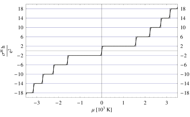
Figure 1: Graphene-like Hall conductivity $\sigma^{H}$ (measured in $e^{2}/h$ units) as a function of chemical potential $\mu$ for $B=1.4*10^{5}$ G, $T=0$ K (dashed line) and $T=15$ K (continuous line). We use $v_{F}=1.0\times 10^{8}$ $cm/s$, which leads to an energy scale (given in units of temperature) $\frac{eB\hbar v_{F}^{2}}{c}\rightarrow$ $\frac{eB\hbar v_{F}^{2}}{ck_{B}^{2}}$(K²) $=8.858\frac{K^{2}}{G}$B(G).

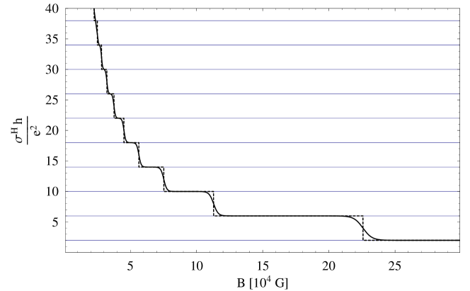
Figure 2: Graphene-like Hall conductivity $\sigma^{H}$ (measured in $e^{2}/h$ units) as a function of magnetic field $B$ for $\mu=2\times 10^{3}$ K, $T=0$ K (dashed line) and $T=15$ K (continuous line).

5 Conclusions

To summarize, we have presented some kinetic properties of the 3D quantum relativistic massless fermion gas in presence of the magnetic field, due to the $C$ non-invariance of the system, and we have obtained the conductivity tensor in the static limit showing that it is completely antisymmetric, since the Ohm conductivity vanish $\sigma_{0}=0$ and the Hall conductivity remains as different from zero at the limit of zero temperature. With the aim to study 2D relativistic system we have introduced an ansatz: the dimensional compactification of $z$-dimension allowing to obtain the Hall conductivity of the system showing the plateaus. From this framework it is possible to obtain the graphene-like half-integer Hall conductivity, if an extra degeneracy factor two, due to the sublattice-valley of graphene, is introduced. Our results are in agreement with the results of [11]-[21] where the Hall conductivity was obtained. The absolute value of graphene conductivity, as well as the 2D relativistic Hall conductivity, exhibits a minimum value of order $e^{2}/h$. This phenomenon is connected to the magnetic catalysis mechanism [28].

References

- [1] Novoselov, K. S. et al., Science 306, 666-669 (2004).
- [2] Novoselov, K. S. et al., Proc. Natl Acad. Sci. USA 102, 10451-10453 (2005).
- [3] P. R. Wallace, Phys. Rev. 71, 622 (1947)
- [4] J. C. Slonczewski and P. R. Weiss, Phys. Rev. 109, 272 (1958).
- [5] J. W. McClure, Phys. Rev. 104, 666 (1956).
- [6] J. Gonzalez, F. Guinea, and M. A. H. Vozmediano, Phys. Rev. B. 59 R2474-7 (1999)
- [7] J. Gonzalez, F. Guinea, and M. A. H. Vozmediano, Phys. Rev. B. 63 134421 (2001).
- [8] Semenoff, G. W., Phys. Rev. Lett. 53, 2449-2452 (1984).
- [9] Fradkin, E., Phys. Rev. B 33, 3263-3268 (1986).
- [10] Haldane, F. D. M., Phys. Rev. Lett. 61, 2015-2018 (1988).
- [11] K. S. Novoselov, A. K. Geim, S. V. Morozov, D. Jiang, M. I. Katsnelson, I. V. Grigorieva1, S. V. Dubonos, A. A. Firsov, Nature 438, 197-200 (2005).
- [12] A. H. Castro Neto, F. Guinea, N. M. R. Peres, K. S. Novoselov and A. K. Geim, Rev. Mod. Phys. 81, 109-162 (2009).
- [13] E. M. C. Abreu, M. A. De Andrade, L. P. G. de Assis, J. A. Helayel-Neto, A. L. M. Nogueira and R. C. Paschoal, JHEP 1105, 001 (2011) [arXiv:1002.2660 [hep-th]].
- [14] E. Fradkin, Field Theories of Condensed Matter Systems (Westview Press, Oxford, 1997). 28.
- [15] G. E. Volovik, The Universe in a Helium Droplet (Clarendon Press, Oxford, 2003).
- [16] M. Khodas,1, 2, . I. A. Zaliznyak,2 and D. E. Kharzeev, Phys. Rev. B 80, 125428 (2009) arXiv:0904.1248v1 [cond-mat.mes-hall]
- [17] V. P. Gusynin, S. G. Sharapov, Phys. Rev. B 71, 125124 (2005).
- [18] V. P. Gusynin, S. G. Sharapov, Phys.Rev. B 73, 245411 (2006).
- [19] V. P. Gusynin, S. G. Sharapov, J. P. Carbotte, Int. J. Mod. Phys. B 21, 4611-4658 (2007).
- [20] V. Juricic, O. Vafek, I. F. Herbut, Phys. Rev. B 82, 235402 (2010).
- [21] C. G. Beneventano, P. Giacconi, E. M. Santangelo and R. Soldati, J. Phys. A 40, F435 (2007) [arXiv:hep-th/0701095].
- [22] A. Raya, E. D. Reyes, J. Phys. A 41, 355401 (2008).
- [23] C. G. Beneventano, E. M. Santangelo, J. Phys. A 41, 164035 (2008).
- [24] C. G. Beneventano, P. Giacconi, E. M. Santangelo, R. Soldati, J. Phys. A 42, 275401 (2009).
- [25] P. Giaconni and R.Soldati, Mod. Phys. Lett, B 24 (2010) 2225.
- [26] E. V. Gorbar, V. P. Gusynin, V. A. Miransky, LowTemp. Phys. 34, 790 (2008).
- [27] Y. Zheng. and T. Ando, Phys. Rev. B 65, 245420 (2002).
- [28] E. V. Gorbar, V. P. Gusynin, V. A. Miransky, I. A. Shovkovy, Phys. Rev. B 78, 085437 (2008).
- [29] V. P. Gusynin, S. G. Sharapov, Phys.Rev. Lett. 95, 146801 (2005).
- [30] Z. Jiang, Y. Zhang, Y.-W. Tan, H.L. Stormer, P. Kim, Solid State Commun. 143, 14 19 (2007).
- [31] Y. Zhang, Y.-W. Tan, H. L. Stormer and P. Kim, Nature 438, 201 204 (2005).
- [32] G.W. Semenoff, Phys. Rev. Lett. 53, 2449 (1984).
- [33] F.D.M. Haldane, Phys. Rev. Lett. 61, 2015 (1988).
- [34] D.V. Khveshchenko, Phys. Rev. Lett. 87, 206401 (2001); ibid. 87, 246802 (2001).
- [35] E.V. Gorbar, V.P. Gusynin, V.A. Miransky, and I.A. Shovkovy, Phys. Rev. B 66, 045108 (2002).
- [36] S.G. Sharapov, V.P. Gusynin, and H. Beck, Phys.Rev. B 69, 075104 (2004).
- [37] I.A. Luk yanchuk and Y. Kopelevich, Phys. Rev. Lett. 93, 166402 (2004).
- [38] K. S. Novoselov, Z. Jiang, Y. Zhang, S. V. Morozov, H. L. Stormer, U. Zeitler, J. C. Maan, G. S. Boebinger, P. Kim, A. K. Geim1, Science 315, 1379 (2007).
- [39] H. Perez Rojas and A. E. Shabad, Annals Phys. 121, 432 (1979).
- [40] H. Perez Rojas and A. E. Shabad, Annals Phys. 138, 1 (1982).
- [41] R. Gonzalez Felipe, A. Perez Martinez and H. Perez Rojas, Mod. Phys. Lett. B 4, 1103 (1990).
- [42] R. Joynt and R. E. Prange, Phys Rev B 29, 3303 (1984)
- [43] A. Cabo and D. Martinez Pedrera, Phys Rev B 67, 245310 (2003)
- [44] Y. Zhang, Z. Jiang, J. P. Small, M. S. Purewal, Y.-W. Tan, M. Fazlollahi, J. D. Chudow, J. A. Jaszczak, H. L. Stormer, P. Kim, Phys. Rev. Lett. 96, 136806 (2006).
- [45] Z. Jiang, Y. Zhang, H. L. Stormer, and P. Kim, Phys. Rev. Lett. 99, 106802 (2007)
- [46] H. Perez Rojas and A. E. Shabad, Kratkie Soob po Fiz. (Lebedev Institute Report, Moscow (New York: Allerton Press) p 16 (1976).
- [47] M.H. Johnson and B. A. Lippmann Phys. Rev. 76 828 (1949)
- [48] A. I. Akhiezer, V. B. Berestetskii, Quantum electrodynamics. (New York: Interscience Publishers) Interscience Publishers, New York (1965).
- [49] V.P. Gusynin, V.A. Miransky, I.A. Shovkovy, Phys.Rev D 52, 4718 (1995)
- [50] C Kittel, Quantum Theory of Solids (New York: John Wiley & Sons, Inc. New York. London) (1963)
- [51] M.I. Katsnelson, K.S. Novoselov Solid State Communications 143 (2007) 3 13