Finite-momentum superfluidity and phase transitions in a $p$-wave resonant Bose gas

Abstract

We study a degenerate two-species gas of bosonic atoms interacting through a $p$-wave Feshbach resonance as for example realized in a ⁸⁵Rb-⁸⁷Rb mixture. We show that in addition to a conventional atomic and a $p$-wave molecular spinor-1 superfluidity at large positive and negative detunings, respectively, the system generically exhibits a finite momentum atomic-molecular superfluidity at intermediate detuning around the unitary point. We analyze the detailed nature of the corresponding phases and the associated quantum and thermal phase transitions.

I Introduction

I.1 Background and Motivation

Since the experimental realization of Bose-Einstein condensation (BEC) in trapped alkali-metal-atom gases cornell.95 ; ketterle.95 , the resulting burgeoning field of degenerate atomic gases has seen an ever-expanding research activity. It has been fueled by the steady advances in new experimental techniques to control and interrogate the continually growing class of degenerate atomic systems. A Feshbach resonance (FR) has been one of these exceptionally fruitful experimental “knobs” that lends exquisite tunability (via magnetic field) of interactions in the ultracold atomic gases. For fermionic trapped gases, it enabled a realization of a fermionic atom-paired $s$-wave superfluidity and exploration of its BEC-BCS crossover and resonant universality regal.04 ; zwierlein.04 ; kinast.04 ; chin.grimm.04 ; hulet.05 ; zwierlein.ketterle.05 ; timmermans.99 ; dieckmann.ketterle.02 ; ohara.thomas.02 ; salomon.03 ; hulet.03 ; duine.stoof.04 ; nozieres.85 ; sademelo.93 ; holland.01 ; ohashi.griffin.02 ; radzihovsky.04 ; levinsen.gurarie.06 ; radzihovsky.07 .

Motivated by the demonstration of $p$-wave FR in ⁴⁰K and ⁶Li, $p$-wave paired fermionic superfluidity has also been extensively explored theoretically ho.diener.05 ; radzihovsky.05 ; radzihovsky.07 ; yip.05 , predicting to exhibit an even richer phenomenology. A recent laboratory production of $p$-wave Feshbach molecules gaebler.07 ; zhang.salomon.04 shows considerable promise toward a realization of $p$-wave fermion-paired superfluidity and the associated rich phenomenology radzihovsky.07 , though substantial challenges of stability remain gaebler.07 ; levinsen.cooper.gurarie.08 .

The bosonic counterparts have also been extensively explored and in fact in the $s$-wave FR case of ⁸⁵Rb wieman.00 predate recent fermionic developments. As was recently emphasized radzihovsky.04.boson ; radzihovsky.08.boson ; romans.04 , in contrast to their fermionic analogs, which undergo a smooth BEC-BCS crossover, resonant bosonic gases are predicted to exhibit magnetic-field- and/or temperature-driven sharp phase transitions between distinct molecular and atomic superfluid phases. One serious impediment to a laboratory realization of this rich physics is the predicted efimov.71 ; mueller.08 and observed wieman.01 instabilities of a resonantly attractive Bose gas sufficiently close to a FR. Nevertheless, a number of features of the phase diagram are expected to be exhibited away from the resonance and/or reflected in the nonequilibrium phenomenology (before the onset of the instability) of a resonant Bose gas. Furthermore, recent extension to an $s$-wave resonant Bose gas in an optical lattice zoller1.10 ; zoller2.10 demonstrated the stabilization through a quantum Zeno mechanism proposed by Rempe rempe.08 , which dates back to Bethe’s bethe analysis of the triplet linewidth in hydrogen. The predictions radzihovsky.04.boson ; radzihovsky.08.boson ; romans.04 ; zoller1.10 ; zoller2.10 have been supported by recent density matrix renormalization group Ejima.Simons.11 , exact diagonalization Bhaseen.Simons.09 , and quantum Monte Carlo Bonnes.Wessel.11 studies, as well extensions to two species Bhaseen.Simons.09 .

Along with the ubiquitous $s$-wave resonances, recent experiments on a ⁸⁵Rb-⁸⁷Rb mixture have demonstrated an interspecies $p$-wave FR at $B=257.8$ G papp.thesis ; papp.08 . Although the consequences of this two-body $p$-wave resonance on the degenerate many-body state of such a gas mixture has not been explored experimentally, it provided the main motivation for our recent RCprl.09 and present studies. We note that closely related studies of BEC in $p$ (and higher) bands in optical lattices have been carried out in Refs. kuklov.06, ; liu.06, .

The rest of the paper is organized as follows. We conclude the Introduction with a summary of our main results and their experimental implications. In Sec. II we introduce a microscopic two-channel $p$-wave FR model for a description of a two-component Bose gas, as for example realized by a ⁸⁵Rb-⁸⁷Rb mixture. Having related the parameters of the model to two-body scattering experiments on a dilute gas, in Sec. III we present a general symmetry-based discussion of phases and associated phase transitions expected in such an atomic gas at finite density. In Sec. IV, by minimizing the corresponding imaginary-time coherent state action, we map out a generic mean-field phase diagram for this system. In Sec. V, we supplement this Landau analysis with a derivation of the corresponding Goldstone-mode Lagrangians and extract from them the low-energy elementary excitations and dispersions characteristic of each phase. The true (beyond-mean-field) nature of the quantum and thermal phase transitions is discussed in Sec. VI. In Sec. VII we study the topological defects, vortices and domain walls, in each of the phases. We make a more direct contact with cold-atom experiments in Sec. VIII by using a local density approximation (LDA) to include the effects of the trapping potential. We close with a brief summary in Sec. IX.

I.2 Summary of results

Before turning to the analysis of the system, we present the main predictions of our work, a small subset of which was previously reported in a Letter RCprl.09 . Our key results are summarized by a FR temperature-detuning phase diagram, illustrated in Fig. 1, and by the properties of the corresponding phases and transitions.

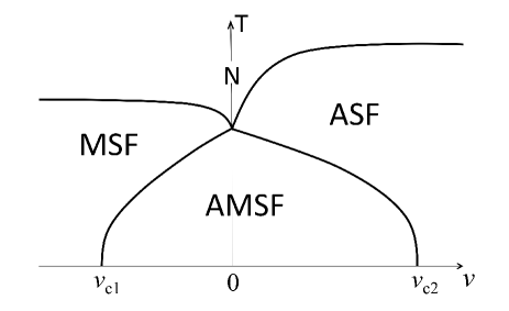
Figure 1: Schematic temperature-detuning phase diagram for a balanced two-species $p$-wave resonant Bose gas. As illustrated, it exhibits atomic (ASF), molecular (MSF), and atomic-molecular (AMSF) superfluid phases. The AMSF state is characterized by a $p$-wave, molecular, and finite-momentum $Q$ (see Fig. 2) atomic superfluidity.

We find that in addition to the normal (i.e., non-superfluid) high-temperature phase, the $p$-wave Feshbach-resonant two-component balanced Bose gas (e.g., equal mixture of ⁸⁵Rb and ⁸⁷Rb atoms) generically exhibits three classes of superfluid phases: atomic (ASF), molecular (MSF), and atomic-molecular (AMSF) condensates, where atoms, $p$-wave molecules, and both are Bose-Einstein-condensed, respectively. Our most interesting finding is that the AMSF phase, sandwiched between (large positive detuning) ASF and (large negative detuning) MSF phases, is necessarily a finite-momentum Q spinor superfluid, akin to (but distinct from) a supersolid Andreev.69 ; Chester.70 ; Leggett.70 ; Kim.Chan.04 . It is characterized by a momentum $\hbar{\textbf{\em Q}}$, with its magnitude

$$Q=\alpha m\sqrt{n_{m}}\sim\sqrt{\gamma_{p}\ell n_{m}}\lesssim\sqrt{\gamma_{p}}/\ell,$$ (1)

tunable with a magnetic field [via FR detuning, $\nu$ that primarily enters through the molecular condensate density $n_{m}(\nu)$], with $\alpha$, $m$, $\ell$, and $\gamma_{p}$, respectively, the FR coupling, atomic mass, average atom spacing, and a dimensionless measure of FR width radzihovsky.07 .

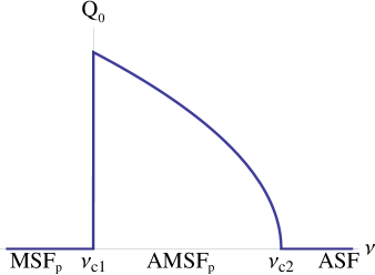
Figure 2: (Color online) Schematic momentum $Q(\nu)$ characteristic of the AMSF (polar) state, ranging between zero and the $p$-wave FR width-dependent value.

As illustrated in the phase diagram (Fig. 1), the ASF appears at a large positive detuning (weak FR attraction) and low temperature, where one of the three combinations (ASF₁, ASF₂, ASF₁₂) of the ⁸⁵Rb and ⁸⁷Rb atoms is Bose-Einstein-condensed into a conventional, uniform superfluid and the $p$-wave ⁸⁵Rb-⁸⁷Rb molecules are energetically costly and therefore appear only as gapped excitations.

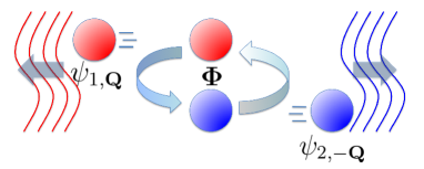
Figure 3: (Color online) A cartoon of a $p$-wave molecule decaying into two oppositely moving species of atoms, illustrating a resonant mechanism for a finite-momentum Q atomic superfluidity (indicated by wavy lines) in the AMSF phase.

In the complementary regime of a large negative detuning, the attraction between two flavors of atoms is sufficiently strong so as to bind them into tight $p$-wave heteromolecules (e.g., ⁸⁵Rb-⁸⁷Rb molecule), which at low temperature condense into a $p$-wave superfluid, with atoms in the species-balanced case existing only as gapped excitations. In this tight-binding molecular regime the gas reduces to a well-explored system of a spinor-$1$ condensate stenger.ketterle.98 ; gorlitz.ketterle.03 ; chang.chapman.04 ; chang.chapman.05 ; kurn.08 ; ho.spinor.98 ; ohmi.machida.98 ; stamperkurn.98 ; matthews.cornell.98 ; bigelow.98 ; ho.yip.00 ; zhou.spinor.01 ; demler.zhou.02 ; barnett.demler.06 ; mukerjee.moore.06 ; mur-petit.06 ; lamacraft.07 ; mukerjee.moore.07 , with the spinor corresponding to the relative orbital angular momentum $\ell=1$ of the two constituent atoms of the $p$-wave molecule. Thus, for negative detuning we predict the existence of $\ell_{z}=0$ “polar” (MSF_p) and $\ell_{z}=\pm 1$ “ferromagnetic” (MSF_fm) molecular $p$-wave superfluid phases, with their relative stability determined by the ratio $a_{0}/a_{2}$ of molecular spin-0 ($a_{0}$) to molecular spin-2 ($a_{2}$) scattering lengths. We find that this ratio and therefore the first-order MSF_p-MSF_fm transition are, in turn, controlled with the $p$-wave FR detuning $\nu$, or equivalently, the atomic $p$-wave scattering volume $v\sim 1/\nu$, tunable with a magnetic field.

We emphasize that (in contrast to the $s$-wave case radzihovsky.04.boson ; radzihovsky.08.boson ; romans.04 ) because a $p$-wave resonance does not couple a uniform atomic condensate to the molecular one, a $p$-wave molecular condensate is not automatically induced inside the ASF state.

The most distinctive signatures of these superfluids should be directly detectable via time-of-flight shadow images, with the ASF exhibiting an atomic condensate peak and the MSF displaying a $p$-wave molecular one. At higher densities in a trap, the bulk phase diagram as a function of the chemical potential (see Fig. 20 and  21) translates into shell structure of distinct phases, which we estimated within the LDA bloch.06 ; campbell.ketterle.06 ; vishveshwara.07 .

In addition to these fairly conventional uniform atomic and molecular BECs, for intermediate detuning around a unitary point we predict the existence of AMSF_p and AMSF_fm phases, characterized by a finite momentum $Q$ atomic condensate kuklov.06 ; RCprl.09 , that is a superposition of the two atomic species. Such a generically supersolid state Andreev.69 ; Chester.70 ; Leggett.70 ; Kim.Chan.04 is always accompanied by a $p$-wave molecular condensate, concomitantly induced through the $p$-wave FR interaction. In addition to exhibiting an off-diagonal long-range order (ODLRO) of an ordinary superfluid the two AMSF_p,fm states (distinguished by the polar versus ferromagnetic nature of their $p$-wave molecular condensates) spontaneously partially break orientational and translational symmetries, akin to polar and smectic liquid crystals degennes.prost.95 and the putative Fulde-Ferrell-Larkin-Ovchinnikov states of imbalanced paired fermions ff.64 ; lo.65 ; hulet.10 ; Sarrao.03 ; mizushima.05 ; SRprl.06 ; SRaop.07 ; RSreview.10 .

As illustrated in Fig. 4, in the AMSF_p state, Q aligns along the quantization axis along which the molecular condensate has a zero projection of its internal $\ell=1$ angular momentum. For the case of the AMSF_fm state, Q lies in the otherwise isotropic plane, transverse to the $p$-wave molecular condensate axis, as illustrated in Fig. 5.

In the narrow FR approximation we find that the AMSF_p,fm states are collinear, characterized by a single Q of a Fulde-Ferrell-like form ff.64 , as opposed to a $+{\textbf{\em Q}}$ and $-{\textbf{\em Q}}$ Larkin-Ovchinnikov-like lo.65 or other more complicated crystalline forms, found in imbalanced paired fermionic systems SRprl.06 ; SRaop.07 ; RSreview.10 . However, because the detailed spatial structure of the AMSF_fm (but not the AMSF_p state) sensitively depends on the interactions (since it spontaneously breaks symmetry transverse to the $\ell_{z}=1$ axis), we do not exclude a more general lattice structure in a more generic beyond-mean-field model, which is best analyzed numerically.

The phase boundaries between this rich variety of phases can be calculated for a narrow FR and in a dilute Bose-gas limit, but are notoriously difficult to estimate in a strongly interacting system, where they can only be qualitatively estimated within a mean-field analysis. In the former case the zero-temperature phase boundaries are given by critical detunings:

$$\nu_{c}^{\rm MSF_{p}-AMSF_{p}} = -\big{(}g_{1}+g_{2}-2g_{am}+\frac{m\alpha^{2}}{\hbar^{2}}\big{)}n_{m},\,\,\,\ \ \ \ \ \ \$$ (2a)

$$\nu_{c}^{\rm AMSF_{p}-ASF} = \big{(}2\lambda-g_{am}+\frac{m\alpha^{2}}{2\hbar^{2}}\big{)}n_{a},\ \ \text{for}\ g_{2}<0,$$

with similar expressions for transitions out of the ferromagnetic phases, which can be found in Eq. (54). Here $g_{i}$’s and $\lambda_{i}$’s are molecular and atomic two-body interaction pseudopotentials, respectively related to the background molecular ($a_{0}^{bg}$ and $a_{2}^{bg}$) and atomic scattering lengths ($a^{bg}_{11}$, $a^{bg}_{22}$, and $a^{bg}_{12}$).

As any neutral superfluid, ASF, MSF, and AMSF are each characterized by Bogoliubov modes, illustrated in Figs. 13, 14, 15, and 16, with long-wavelength acoustic “sound” dispersions,

$$E^{\rm B}_{\sigma}({\bf k})\approx c_{\sigma}\hbar k,$$ (3)

where $c_{\sigma}$ (with $\sigma=$ASF_1,2,12, MSF_p,fm, AMSF_p,fm) are the associated sound speeds with standard Bogoliubov form $c_{\sigma}\approx\sqrt{g_{\sigma}n_{\sigma}/2m}$. In each of these SF states one Bogoliubov mode (and only one in the ASF_i states) corresponds to the overall condensate phase fluctuations. In addition, the MSF_p exhibits two degenerate “transverse” Bogoliubov orientational acoustic modes. The MSF_fm is also additionally characterized by one “ferromagnetic” spin-wave mode, $E_{k}^{\rm MSF_{fm}}\sim k^{2}$ and one gapped mode, consistent with the characteristics of a conventional spinor-1 condensate ho.spinor.98 ; ohmi.machida.98 .

Because MSF_p,fm’s are paired MSFs, they also exhibit gapped single atomlike quasiparticles (akin to Bogoliubov excitations in a fermionic paired BCS state) that do not carry a definite atom number. These single-particle excitations are “squeezed” by the presence of the molecular condensate, offering a mechanism to realize atomic squeezed states kimble.90 , which can be measured by interference experiments, similar to those reported in Ref. kasevich.01, . The low-energy nature of these single-atom excitations is guaranteed by the vanishing of the gap at the MSF-AMSF transition at $\nu_{c}^{\rm MSF_{p,fm}-AMSF_{p,fm}}$, with $E^{\rm gap}_{\rm MSF}(\nu_{c})=0$.

We also note that inside the MSF_p,fm, for $\nu>\nu^{\rm p,fm}_{*}=-(g_{\rm p,fm}+C_{\rm p,fm}m\alpha^{2}/\hbar^{2})n_{m}$, where $C_{\rm p,fm}=2,1$ for polar and ferromagnetic phases, respectively, the minimum of the single-atom excitations (that for $\nu<\nu_{*}$ is at $k=0$) shifts to a finite momentum, $k\approx Q$. This is a precursor of the atomic gap-closing MSF-AMSF transition at $\nu_{c}^{\rm MSF-AMSF}$, where atoms also Bose condense at finite momentum $Q$.

We predict that in addition to the conventional Bogoliubov superfluid mode associated with the phase common to the atomic and molecular condensates, the AMSF also exhibits a Goldstone mode corresponding to the fluctuation of a relative phase between the two atomic condensate components. Furthermore, a spatially periodic, collinear AMSF state, characterized by at least $\pm{\textbf{\em Q}}$ momenta (but not just single Q) further exhibits the condensate phonon mode $u$ corresponding to the difference between phases of the $\pm{\textbf{\em Q}}$ condensate components, akin to the Larkin-Ovchinnikov state lo.65 ; radzihovsky.vishwanath.08 ; FFLOlongLeo .

For the single Q AMSF states, we predict the smecticlike “phonon” spectra in the polar and ferromagnetic cases,

$$\omega_{\rm AMSF_{p}}({\textbf{\em k}}) = \sqrt{(Bk_{z}^{2}+Kk^{4}_{\perp})/\chi_{-}},$$ (4a)

$$\omega_{\rm AMSF_{fm}}({\textbf{\em k}}) = \sqrt{(Bk_{z}^{2}+k^{2}(K_{x}k_{x}^{2}+K_{y}k_{y}^{2}))/\chi_{-}},$$

as well as the conventional Bogoliubov modes associated with superfluid order, and an orientational mode $\omega_{\rm fm}^{\gamma}$, associated with orientational symmetry breaking in AMSF_fm

$$\omega_{+p}({\textbf{\em k}})= \sqrt{\frac{2\rho_{s}}{\chi_{+}m}}k,$$ (5a)

$$\omega_{\rm fm}^{\gamma}({\textbf{\em k}})= \sqrt{\frac{Jk^{2}\left[Bk^{2}_{z}+k^{2}(K_{x}k_{x}^{2}+K_{y}k_{y}^{2})\right]}{J\chi_{-}k^{2}+\kappa^{2}k_{y}^{2}}},$$ (5b)

where $B=\frac{2\hbar^{2}n_{a}}{m}$, $K=K_{x}=2K_{y}=\frac{\hbar^{6}}{2m^{3}\alpha^{2}}$, $J=\frac{\hbar^{2}n_{m}}{4m}$, $\kappa=\frac{\hbar^{2}\sqrt{n_{m}}}{\alpha m}$, and $\chi_{-}^{-1}=\frac{1}{2}(\lambda-\lambda_{12})$.

Having summarized the results of our study, we next turn to the definition of the two-component $p$-wave resonant Bose-gas model, followed by its detailed analysis.

II Model

We study a gas mixture of two distinguishable bosonic atoms (e.g., ⁸⁵Rb, ⁸⁷Rb) papp.08 , created by field operators $\psi_{\sigma}^{\dagger}({\bf r})=\left(\psi_{1}^{\dagger}({\bf r}),\psi_{2}^{\dagger}({\bf r})\right)$ and interacting through a $p$-wave FR associated with a tunable “closed”-channel bound state. The corresponding $p$-wave ($\ell=1$) closed-channel hetero-molecule (e.g., ⁸⁵Rb-⁸⁷Rb) is created by a Cartesian vector field operator ${\bm{\phi}}^{\dagger}({\bf r})=(\phi_{x}^{\dagger},\phi_{y}^{\dagger},\phi^{\dagger}_{z})$, related to $\phi_{\pm}^{\dagger}=(\phi_{x}^{\dagger}\pm i\phi_{y}^{\dagger})/\sqrt{2},\phi_{z}^{\dagger}=\phi_{z}^{\dagger}$ operators, which create closed-channel molecules in the $\ell_{z}=\pm 1,0$ eigenstates, respectively. This system is governed by a grand-canonical Hamiltonian density (with $\hbar=1$ throughout),

$${\cal H} = \sum_{\sigma=1,2}\hat{\psi}_{\sigma}^{{\dagger}}\hat{\varepsilon}_{\sigma}\hat{\psi}_{\sigma}+\hat{\bm{\phi}}^{{\dagger}}\cdot\hat{\omega}\cdot\hat{\bm{\phi}}+{\cal H}_{bg}$$

$$+\frac{\alpha}{2}\left(\hat{\bm{\phi}}^{{\dagger}}\cdot\left[\hat{\psi}_{1}(-i{\bm{\nabla}})\hat{\psi}_{2}-\hat{\psi}_{2}(-i{\bm{\nabla}})\hat{\psi}_{1}\right]+h.c.\right),$$

where single-particle atomic and molecular Hamiltonians are given by

$$\hat{\varepsilon}_{\sigma} = -\frac{1}{2m}{\bm{\nabla}}^{2}-\mu_{\sigma},$$ (7a)

$$\hat{\omega} = -\frac{1}{4m}{\bm{\nabla}}^{2}-\mu_{m},$$ (7b)

with the effective molecular chemical potential,

$$\mu_{m}=\mu_{1}+\mu_{2}-\nu,$$ (8)

adjustable by a magnetic-field-dependent detuning $\nu$, the latter being the rest energy of the closed-channel molecule relative to a pair of open-channel atoms. For simplicity we have taken atomic masses to be identical (a good approximation for the ⁸⁵Rb-⁸⁷Rb mixture that we have in mind) and will focus on the balanced case of $\mu_{1}=\mu_{2}=\mu$, with $\mu$ fixing the total number of ⁸⁵Rb and ⁸⁷Rb atoms, whether in the (open-channel) atomic or (closed-channel) molecular form. The FR interaction encodes a coherent interconversion between a pair of open-channel atoms $1,2$ (in a singlet combination of $1,2$ labels, as required by bosonic statistics) and a closed-channel $p$-wave molecule, with amplitude $\alpha$ commentFRequalmass .

The FR coupling $\alpha$ and detuning $\nu$ are fixed experimentally through measurements of the low-energy two-atom $p$-wave scattering amplitude regal.03 ; gaebler.07 ,

$$f_{p}(k)=\frac{k^{2}}{-v^{-1}+\frac{1}{2}k_{0}k^{2}-ik^{3}},$$ (9)

where $v$ is the scattering volume (tunable via magnetic field dependent detuning $\nu$) and $k_{0}$ (negative for the FR case) is the characteristic wave vector landau.QM ; radzihovsky.07 ,

$$v^{-1} = -\frac{6\pi}{m\alpha^{2}}(\nu-c_{1}),$$ (10a)

$$k_{0} = -\frac{12\pi}{m^{2}\alpha^{2}}(1+c_{2}),$$ (10b)

respectively analogous to the scattering length $a$ and the effective range $r_{0}$ in $s$-wave scattering case. In the above equations, constants $c_{1,2}$ are determined by the details of the $p$-wave interaction at short scales, which in the pseudopotential model above are given by radzihovsky.07

$$c_{1} = \frac{m\alpha^{2}}{9\pi^{2}}\Lambda^{3},$$ (11a)

$$c_{2} = \frac{m^{2}\alpha^{2}}{3\pi^{2}}\Lambda,$$ (11b)

where $\Lambda=2\pi/d$ is the inverse size of the closed-channel molecular bound state, on the order of the interatomic potential range.

The $p$-wave resonance and bound-state energy are determined by the poles of $f_{p}(k)$. At low energies (where $ik^{3}$ can be neglected) the energy of the pole is given by

$$E_{p}=\frac{k_{p}^{2}}{2m}\approx-\frac{1}{mv|k_{0}|},$$ (12)

which is real and negative and thus is a bound-state energy for $v>0$ (negative detuning) and a finite lifetime resonance for $v<0$ (positive detuning).

In the above, for simplicity we have focused on a rotationally invariant FR interaction, with $\hat{\omega}$ and $\alpha$ independent of the molecular component $i$. This is an approximation for our system of interest, the ⁸⁵Rb-⁸⁷Rb mixture, where, indeed, the $p$-wave FR around $B=257.8$ G papp.thesis ; papp.08 is split into a doublet by approximately $\Delta B=0.6$ G, similar to the fermionic case of ⁴⁰K regal.03 ; gaebler.07 ; radzihovsky.05 ; radzihovsky.07 . We leave the more realistic, richer case for future studies.

The background (nonresonant) interaction density

$${\cal H}_{bg}={\cal H}_{a}+{\cal H}_{m}+{\cal H}_{am}$$ (13)

is given by

$${\cal H}_{a} = \sum_{\sigma=1,2}\frac{\lambda_{\sigma}}{2}\hat{\psi}^{{\dagger}2}_{\sigma}\hat{\psi}^{2}_{\sigma}+\lambda_{12}\hat{\psi}^{{\dagger}}_{1}\hat{\psi}^{{\dagger}}_{2}\hat{\psi}_{2}\hat{\psi}_{1},$$ (14a)

$${\cal H}_{m} = \frac{g_{1}}{2}(\hat{\bm{\phi}}^{{\dagger}}\cdot\hat{\bm{\phi}})^{2}+\frac{g_{2}}{2}|\hat{\bm{\phi}}\cdot\hat{\bm{\phi}}|^{2},$$ (14b)

$${\cal H}_{am} = \sum_{\sigma=1,2}g_{am}\hat{\psi}^{{\dagger}}_{\sigma}\hat{\bm{\phi}}^{\dagger}\cdot\hat{\bm{\phi}}\hat{\psi}_{\sigma},$$ (14c)

where coupling constants $\lambda_{\sigma}$, $\lambda_{12}$, $g_{1,2}$, $g_{am}$ are related to the corresponding background $s$-wave scattering lengths ($a_{1}$, $a_{2}$, etc.) in a standard way and thus are fixed experimentally through measurements on the gas in a dilute limit regal.04 . Correspondingly, we take these background $s$-wave couplings to be independent of the $p$-wave detuning, an approximation that we expect to be quantitatively valid in the narrow resonance and/or dilute limits considered here. A miscibility of a two-component atomic gas requires greene.97

$$a_{1}a_{2}>a_{12}^{2}$$ (15)

which may be problematic for the case of ⁸⁵Rb-⁸⁷Rb due to the negative background scattering length of ⁸⁵Rb.

The molecular interaction couplings $g_{1}$, $g_{2}$ (set by the $L=0$ and $L=2$ channels of $p$-wave molecule-molecule scattering), and $g_{am}$ can be derived from a combination of $s$-wave atom-atom ($\lambda_{\sigma}$) and $p$-wave FR ($\alpha$) interactions. We present lowest order of this analysis in Sec.IV.4.3, which shows that these parameters can, in principle, be tuned via a magnetic field through the $p$-wave FR detuning $\nu$.

The above two-channel model [Eq. (II)] faithfully captures the low-energy $p$-wave resonant and $s$-wave nonresonant scattering phenomenology of the ⁸⁵Rb-⁸⁷Rb $p$-wave Feshbach-resonant mixture papp.08 . Its analysis at nonzero balanced atomic densities, which is our focus here, leads to the predictions summarized in the previous section.

II.0.1 Lattice model

As discussed in the Introduction, based on the experience for the $s$-wave case radzihovsky.04.boson ; radzihovsky.08.boson ; romans.04 ; lee.lee.04 , it is likely that a stable realization of the above continuum $p$-wave resonant two-species bosonic model will require an introduction of an optical lattice zoller1.10 ; zoller2.10 . This leads to a two-component atomic Hubbard model, with standard tight-binding atomic and molecular lattice-hopping kinetic energies, density-density interactions, and a lattice projection of the $p$-wave Feshbach resonant coupling that in a single-band Wannier basis is given by

$${\cal H}_{\rm FR_{p}}^{\rm lattice} =\frac{\alpha}{2}\sum_{{\bf r}_{i},\alpha}b_{\alpha{\bf r}_{i}}^{\dagger}(a_{1,{\bf r}_{i}}a_{2,{\bf r}_{i}-{{\bm{\delta}}_{\alpha}}}-a_{1,{\bf r}_{i}}a_{2,{\bf r}_{i}+{{\bm{\delta}}_{\alpha}}})+h.c.,$$ (16)

where, for example, on a cubic lattice, ${\bm{\delta}}_{\alpha}$ are lattice vectors. A related finite angular-momentum FR lattice model was proposed and studied in an interesting paper by Kuklov kuklov.06 , predicting a robust $p$-wave atomic condensate in an optical lattice. As usualFisherWeichmanGrinsteinFisher , at low lattice filling this lattice model reproduces the phenomenology of the continuum model. As an additional qualitative feature, at commensurate lattice fillings we also expect it to admit a rich variety of zero-temperature Mott insulating phases and quantum phase transitions from them to the superfluid ground states exhibited by the continuum system studied here. We leave the detailed analysis of the lattice model to future studies.

II.0.2 Coherence-state formulation of thermodynamics

With the model defined by $\hat{\cal H}$ [Eqs. (II), (13), and (14)], the thermodynamics as a function of the chemical potential $\mu$ (or equivalently total atom density, $n$), detuning $\nu$, and temperature $T$ can be worked out in a standard way by computing the partition function $Z=\text{Tr}[e^{-\beta\hat{H}}]$ ($\beta\equiv 1/k_{B}T$) and the corresponding free energy $F=-k_{B}T\ln Z$. The trace over quantum mechanical many-body states can be conveniently reformulated in terms of an imaginary-time ($\tau=it$) functional integral over coherent-state atomic, $\psi_{\sigma}(\tau,{\bf r})$ ($\sigma=1,2$), and molecular, $\bm{\phi}(\tau,{\bf r})$, fields:

$$Z=\int D\psi^{*}_{\sigma}D\psi_{\sigma}D{\bm{\phi}^{*}}D\bm{\phi}\,e^{-S},$$ (17)

where the imaginary-time action is given by Negele.Orland

$$S= \int_{0}^{\beta}d\tau\int d{{\bf r}}\bigg{[}\psi^{*}_{\sigma}\partial_{\tau}\psi_{\sigma}+\bm{\phi}^{*}\cdot\partial_{\tau}\bm{\phi}$$

$$+{\cal H}(\psi_{\sigma}^{*},\psi_{\sigma},\bm{\phi}^{*},\bm{\phi})\bigg{]},$$ (18a)

$$= \int_{0}^{\beta}d\tau\int d{{\bf r}}{\cal L}.$$ (18b)

The Lagrangian density is given by

$${\cal L} = \psi^{*}_{\sigma}(\partial_{\tau}-\frac{\nabla^{2}}{2m}-\mu_{\sigma})\psi_{\sigma}+\bm{\phi}^{*}\cdot(\partial_{\tau}-\frac{\nabla^{2}}{4m}-\mu_{m})\cdot\bm{\phi}+\frac{\lambda_{\sigma}}{2}|\psi_{\sigma}|^{4}$$ (19)

$$+ \lambda_{12}|\psi_{1}|^{2}|\psi_{2}|^{2}+g_{am}\left(|\psi_{1}|^{2}+|\psi_{2}|^{2}\right)|{\bm{\phi}}|^{2}+\frac{g_{1}}{2}|{\bm{\phi}}^{*}\cdot{\bm{\phi}}|^{2}+\frac{g_{2}}{2}|{\bm{\phi}}\cdot{\bm{\phi}}|^{2}$$

$$+ \frac{\alpha}{2}\left({\bm{\phi}}^{*}\cdot\left[\psi_{1}(-i{\bm{\nabla}})\psi_{2}-\psi_{2}(-i{\bm{\nabla}})\psi_{1}\right]+c.c.\right).$$

Above (and throughout), the summation over a repeated index, as for $\sigma$ in the first term, is implied.

We note that closely related models also arise in completely distinct physical contexts. These include quantum magnets that exhibit incommensurate spin-liquid states sachdev and bosonic atoms in the presence of spin-orbit interactions huizhai .

The associated coherent-state action $S$ is the basis of all of our analysis in subsequent sections for the computation of the phase diagram, the nature of the phases and excitations in each of the corresponding phases of a $p$-wave resonant Bose gas.

III Phases and their symmetries

Before turning to a microscopic analysis, it is instructive to consider the nature of the expected phases, corresponding Goldstone modes and associated phase transitions based on the underlying symmetries and their spontaneous breaking.

The fully disordered symmetric state of our two-component Bose gas confined inside an isotropic and homogeneous boxtrap trap exhibits the $U_{N}(1)\otimes U_{\Delta N}(1)\otimes O(3)\otimes T_{r}\otimes{\cal T}$ symmetries. The first two $U(1)$ groups are associated with the total (whether in atomic or molecular form) atom number $N=N_{1}+N_{2}+2N_{m}$ and the atom species number difference $\Delta N=N_{1}-N_{2}$ conservations. The $O(3)\times T_{r}$ symmetries correspond to the Euclidean group of three-dimensional rotations and translations (in a trap-free case), and ${\cal T}$ is a symmetry of time reversal.

Since our system is composed of bosonic atoms and molecules confined to a large trap commentNoMI , at sufficiently low temperature we expect it to be a superfluid that in three dimensions exhibits BEC, characterized by complex scalar atomic, $\Psi_{\sigma}$, and/or $3$-vector molecular, ${\bm{\Phi}}$, order parameters. Thus, in addition to the high-temperature normal (non-superfluid) state, where the above order parameters all vanish and the full symmetry $U_{N}(1)\otimes U_{\Delta N}(1)\otimes O(3)\otimes{\cal T}\otimes T_{r}$ is manifest commentSymmetries , at low temperature we expect the system to exhibit three classes of SF phases,

1. Atomic Superfluid (ASF), $\Psi_{\sigma}\neq 0$ and ${\bm{\Phi}}=0$,

2. Molecular Superfluid (MSF), $\Psi_{\sigma}=0$ and ${\bm{\Phi}}\neq 0$,

3. Atomic Molecular Superfluid (AMSF), $\Psi_{\sigma}\neq 0$ and ${\bm{\Phi}}\neq 0$,

that spontaneously break one or more of the above symmetries. Although these phase classes resemble the previously studied phases of an $s$-wave Feshbach-resonant system radzihovsky.04.boson ; radzihovsky.08.boson ; romans.04 , as is clear in the following discussion, there are important qualitative differences.

III.1 Atomic superfluid phases, ASF

At large positive detuning $\nu$ it is clear that the molecules are gapped and all atoms are in the unpaired open channel. In this regime, the gapped molecules can be neglected (or integrated out) and the Hamiltonian (II) reduces to that of two bosonic atom species, that can exhibit BEC characterized by $\Psi_{1}$, $\Psi_{2}$ condensates. Such a two-component system is characterized by two types of phase-diagram topologies and has been extensively studied in the statistical physics community LiuFisher ; KNF ; Vicari .

For $a_{1}a_{2}>a_{12}^{2}$ it admits three ASF phases,

1. ASF₁ ($\Psi_{1}\neq 0,\Psi_{2}=0$),

2. ASF₂ ($\Psi_{1}=0,\Psi_{2}\neq 0$),

3. ASF₁₂ ($\Psi_{1}\neq 0,\Psi_{2}\neq 0$),

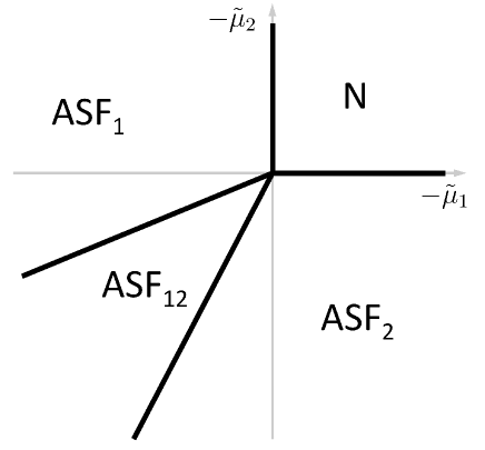
Figure 6: Mean-field phase diagram of a $p$-wave resonant two-component Bose gas for large positive detuning. Molecules are gapped, reducing the system to a conventional two-component Bose gas, for $\lambda_{1}\lambda_{2}>\lambda_{12}^{2}$ displaying three types of ASF phases.

with ASF₁ and ASF₂ separated from ASF₁₂ and the normal phases by continuous phase transitions driven by temperature and density, or atomic polarization (or equivalently the chemical potential imbalance) as illustrated in a mean-field phase diagram (Fig. 6). These phases clearly break $U_{1}(1)$, $U_{2}(1)$, or both of these symmetries, respectively, and are therefore expected to exhibit conventional Bogoliubov modes corresponding to these $U(1)$ symmetries.

Alternatively, for $a_{1}a_{2}<a_{12}^{2}$, the ASF₁₂ state is unstable, with ASF₁ and ASF₂ separated by a first-order transition and the associated phase separation visible in a trap.

We emphasize that, in contrast to the $s$-wave FR bosonic system (where atomic condensation necessarily induces a molecular one, and therefore the ASF phase is not qualitatively distinct from the $s$-wave AMSF phase, being separated from it by a smooth crossover) radzihovsky.04.boson ; radzihovsky.08.boson ; romans.04 , for a $p$-wave FR, above $k=0$ atomic ASF condensates do not automatically induce a $p$-wave molecular condensate since for $k=0$ the $p$-wave FR coupling vanishes. Thus, the ASF class of phases is qualitatively distinct from the AMSF class that we discuss below.

III.2 Molecular superfluid phases, MSF

In the opposite limit of a large negative detuning, atoms are gapped, tightly bound into heteromolecules that at low temperature condense into a $p$-wave MSF. In this regime of atomic vacuum, the gas reduces to that of interacting $p$-wave molecules, a system quite clearly isomorphic to that of the extensively studied $F=1$ spinor condensate kurn.08 ; ho.spinor.98 ; ohmi.machida.98 ; bigelow.98 ; ho.yip.00 ; zhou.spinor.01 ; demler.zhou.02 ; barnett.demler.06 ; mukerjee.moore.06 , with the hyperfine spin $F$ here replaced by the orbital $\ell=1$ angular momentum of two constituent atoms.

Like $F=1$ spinor condensates, the $p$-wave MSF can exhibit two distinct phases depending on the sign of the renormalized interaction coupling $g_{2}$ in Eq. (14b), or equivalently the sign of the difference $a_{0}^{(m)}-a_{2}^{(m)}$ of the molecular $L=0$ and $L=2$ channels $s$-wave scattering lengths comment_g .

III.2.1 Ferromagnetic molecular superfluid, MSF_fm

For $g_{2}>0$ the ground state is the so-called “ferromagnetic” molecular superfluid, MSF_fm, characterized by an order parameter, ${\bm{\Phi}}=\frac{\Phi_{\rm fm}}{\sqrt{2}}({\hat{\bm{n}}}\pm i{\hat{\bm{m}}})$, with ${\hat{\bm{n}}}$, ${\hat{\bm{m}}}$, $\hat{\bm{\ell}}\equiv{\hat{\bm{n}}}\times{\hat{\bm{m}}}$ a real orthonormal triad, $\Phi_{\rm fm}$ a real amplitude, and the state corresponding to $\ell_{z}=\pm 1$ projection of the internal molecular orbital angular momentum along the $\hat{\bm{\ell}}$ axis. MSF_fm spontaneously breaks the time reversal, the $O(3)$ rotational and the global gauge symmetry $U_{N}(1)$, the latter corresponding to a total atom number $N$ conservation. Inside MSF_fm the low-energy order parameter manifold is that of the $O(3)=SU(2)/\mathbb{Z}_{2}$ group, corresponding to orientations of the orthonormal triad ${\hat{\bm{n}}},{\hat{\bm{m}}},\hat{\bm{\ell}}$.

As its hyperfine spinor-condensate cousin, MSF_fm, exhibits two gapless Goldstone modes, one linear ($\propto k$) Bogoliubov mode associating with the broken global gauge symmetry and another quadratic ($\propto k^{2}$) corresponding to the ferromagnetic order, with associated spin waves ho.spinor.98 reflecting the precessional FM dynamics.

III.2.2 Polar molecular superfluid, MSF_p

Alternatively, for $g_{2}<0$ the ground state is the so-called “polar” commentTerminology molecular superfluid, MSF_p, characterized by a (collinear) order parameter, ${\bm{\Phi}}=\Phi_{\rm p}e^{i\varphi}{\hat{\bm{n}}}$, with ${\hat{\bm{n}}}$ a real unit vector, $\varphi$ a (real) phase, and $\Phi_{\rm p}$ a (real) order-parameter amplitude, with the state corresponding to $\ell_{z}=0$ projection of the internal molecular orbital angular momentum along ${\hat{\bm{n}}}$. MSF_p clearly spontaneously breaks rotational symmetry by its choice of the $\ell_{z}=0$ quantization axis ${\hat{\bm{n}}}$ and the global gauge symmetry, corresponding to a total atom number conservation. The low-energy order parameter manifold that characterizes MSF_p is given by the coset space $(U(1)\otimes S_{2})/\mathbb{Z}_{2}$, admitting half-integer “charge” vortices mukerjee.moore.06 akin to (but distinct from) the $s$-wave MSF radzihovsky.04.boson ; romans.04 ; radzihovsky.08.boson .

As we demonstrate explicitly in Sec. V, based on symmetry we expect the polar MSF_p state to exhibit three gapless Bogoliubov-like modes. One corresponds to the breaking of the global atom number conservation and two are associated with the breaking of rotational $O(3)$ symmetry ho.spinor.98 .

III.3 Atomic-molecular superfluid phases, AMSF

As detuning is increased from large negative values of the MSF_p,fm phases, for intermediate $\nu$ the gap to atomic excitations decreases, closing at a critical value of $\nu_{c}^{\rm MSF-AMSF}$ at which, in addition, an atomic BEC takes place. General arguments show that this precedes the atomic condensation in the absence of FR coupling; that is, $\nu_{c}^{\rm MSF-AMSF}(\alpha)<\nu_{c}^{\rm MSF-AMSF}(0)$. The features of this MSF-AMSF transition and the AMSF phase are derived from the fact that at these intermediate detuning, the atomic condensation necessarily takes place at a finite momentum $k=Q$, set by a balance of the $p$-wave FR hybridization and the atomic kinetic energies.

We emphasize that in contrast to the $s$-wave Feshbach-resonant bosons radzihovsky.04.boson ; radzihovsky.08.boson , for which an atomic condensate necessarily induces a molecular condensate, thereby erasing a qualitative distinction between the AMSF and ASF states, for the $p$-wave case, ASF and AMSF phases are qualitatively distinct radzihovsky.04.boson . The latter is ensured by the momentum-dependent nature of the $p$-wave coupling that breaks spatial rotational invariance and vanishes for ${\textbf{\em Q}}=0$.

As with other crystalline states of matter Chaikin.Lubensky ; ff.64 ; lo.65 , the detailed nature of the resulting AMSF states depends on the symmetry of the crystalline order, set by the reciprocal lattice vectors, ${\textbf{\em Q}}_{n}$, at which condensation takes place. Determined by a detailed nature of interactions and fluctuations, typically the nature of crystalline order is challenging to determine generically. Here we focus on the collinear states, with a parallel set of ${\textbf{\em Q}}_{n}=n{\textbf{\em Q}}$, that in the present system can be generically shown to be energetically preferred in the AMSF_p state. There are two possible classes of such collinear states, which are bosonic condensate analogs of the Fulde-Ferrell (FF) ff.64 and Larkin-Ovchinnikov (LO) lo.65 states, extensively studied in fermionic paired superconductors and superfluids SRprl.06 ; SRaop.07 ; RSreview.10 . The qualitative features of these classes of finite-momentum superfluids are well captured by two simplest representative states, one with a single Q and the other with a pair of $\pm{\textbf{\em Q}}$ condensate, which we respectively denote as “vector” (AMSF^v) and “smectic” (AMSF^s). With a choice of Q the AMSF^v,s states both break spatial rotational symmetry. However, they are qualitatively distinguished by the AMSF^v also spontaneously breaking the time-reversal symmetry, while remaining homogeneous, and the AMSF^s instead also breaking the translational symmetry along Q, while remaining symmetric under the time reversal. Because within a mean-field theory analysis it is the former, vector state that appears to be favored, for simplicity we focus on the single Q AMSF states.

The nature and symmetries of these AMSF states furthermore qualitatively depends on the parent MSF, with AMSF_fm and AMSF_p as two possibilities depending on the sign of the renormalized interaction coupling $g_{2}$. In addition to the symmetries already broken in its MSF parent, by virtue of atomic condensation the AMSF state breaks the remaining $U_{\Delta N}(1)$ global gauge symmetry associated with the conservation of the difference in atom species number, $\Delta N$. Other symmetries that it breaks depend on the detailed structure of the AMSF${}_{\rm fm,p}^{v,s}$ states.

III.3.1 Polar atomic-molecular superfluid, AMSF_p

The AMSF_p emerges from the MSF_p. As we see in the next section, in the AMSF_p the finite-momentum atomic condensate orders with Q along the molecular condensate field $\bm{\Phi}$, and therefore (as illustrated in Fig.4) for a single Q the vector superfluid does not break any additional spatial symmetries. With the molecular quantization axis, $\bm{\Phi}$ locked to the atomic condensate momentum Q, on general symmetry grounds (simultaneous rotations of $\bm{\Phi}$ and Q is a zero-energy Goldstone mode), we expect and indeed find that (see Sec. V.3) the superfluid phase will be characterized by a smectic Chaikin.Lubensky Goldstone-mode Hamiltonian. The AMSF${}_{\rm p}^{s}$ superfluid, in addition breaks translational symmetry along $\bm{\Phi}$, with low-energy fluctuations about this state described by a smectic phonon $u$ and a superfluid phase $\varphi$ Goldstone modes.

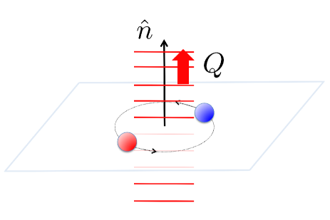
Figure 4: (Color online) Schematic of the AMSF_p state. The thick arrow indicates the atomic condensate momentum Q and the $\hat{n}$ arrow denotes the quantization axis along which the projection of molecular internal orbital angular momentum vanishes.

III.3.2 Ferromagnetic atomic-molecular superfluid, AMSF_fm

In contrast, a finite-momentum atomic condensation from the MSF_fm leads to the AMSF_fm. In this state, a $p$-wave Feshbach resonant interaction leads to the energetic preference for a transverse orientation of the atomic condensate momentum Q to the molecular quantization axis, $\hat{\bm{\ell}}=\hat{\bm{n}}\times\hat{\bm{m}}$. Consequently, as illustrated in Fig. 5, the AMSF_fm state breaks additional orientational symmetry of the uniaxial molecular state in the plane transverse to the molecular quantization axis $\hat{\bm{\ell}}$. That is, the AMSF_fm state is a biaxial nematic superfluid defined by Q and $\hat{\bm{\ell}}$ axes, with the superfluid phase described by a smectic Chaikin.Lubensky Goldstone-mode Hamiltonian akin to that of the FF state FFLOlongLeo . The latter form is enforced by the symmetry associated with a simultaneous reorientation of atomic momentum Q and molecular gauge transformation. The biaxial AMSF${}_{\rm fm}^{s}$ superfluid, in addition breaks translational symmetry along Q, with low-energy fluctuations about this state described by two Goldstone modes, which are a smectic phonon $u$ and a superfluid phase $\varphi$.

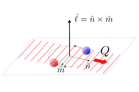
Figure 5: (Color online) Schematic of the AMSF_fm state. The thick arrow indicates the atomic condensate momentum Q, lying in the plane transverse to the quantization axis $\hat{\bm{\ell}}$, along which the projection of the molecular internal orbital angular momentum is $\ell_{z}=+1$.

IV Mean Field Theory

Our main goal in this paper is to establish the phase diagram and nature of phase transitions exhibited by the $p$-wave Feshbach-resonant two-component Bose gas. This requires a minimization of the free energy which, in the presence of interactions and fluctuations is a nontrivial function of a number of systems’ physical parameters. However, outside the critical region, inside each phase where fluctuations are small commentNearTc , we can approximate the Landau free-energy functional $F[\Psi_{\sigma},{\bm{\Phi}}]$ by replacing the atomic and molecular coherent state fields with the classical order parameters, $\Psi_{\sigma}({\bf r})$, ${\bm{\Phi}}({\bf r})$, that minimize the action $S$ via the saddle-point method. In the simplest approximation, the Landau free-energy functional $F[\Psi_{\sigma},{\bm{\Phi}}]$ takes the form identical to $H[\hat{\psi}_{\sigma},\hat{\bm{\phi}}]$,

$$F[\Psi_{\sigma},{\bm{\Phi}}]= \int d^{3}r\Bigg{[}\sum_{\sigma=1,2}\Big{(}\Psi_{\sigma}^{*}\tilde{\varepsilon}_{\sigma}\Psi_{\sigma}+\frac{\tilde{\lambda}_{\sigma}}{2}|\Psi_{\sigma}|^{4}\Big{)}$$

$$+ \tilde{\lambda}_{12}|\Psi_{1}|^{2}|\Psi_{2}|^{2}+\tilde{g}_{am}\left(|\Psi_{1}|^{2}+|\Psi_{2}|^{2}\right)|{\bm{\Phi}}|^{2}$$

$$+ {\bm{\Phi}}^{*}\cdot\tilde{\omega}\cdot{\bm{\Phi}}+\frac{\tilde{g}_{1}}{2}|{\bm{\Phi}}^{*}\cdot{\bm{\Phi}}|^{2}+\frac{\tilde{g}_{2}}{2}|{\bm{\Phi}}\cdot{\bm{\Phi}}|^{2}$$

$$+ \frac{\tilde{\alpha}}{2}\left({\bm{\Phi}}^{*}\cdot\left[\Psi_{1}(-i{\bm{\nabla}})\Psi_{2}-\Psi_{2}(-i{\bm{\nabla}})\Psi_{1})\right]+c.c.\right)\Bigg{]},$$ (20)

with the effective couplings $(\tilde{\mu}_{\sigma},\tilde{\mu}_{m},\tilde{\lambda}_{\sigma},\dots)$, which are functions of the microscopic parameters $(\mu_{\sigma},\mu_{m},\lambda_{\sigma},\dots)$ in Eq. (II), encoding all the complexity of the fluctuations and interactions on short scales. Though nontrivial, these parameters are, in principle, derivable from the Hamiltonian. However, we are not concerned with this aspect of the problem. Instead, our goal is to capture the qualitative form of the phase diagram, taking fluctuations into account only when they qualitatively modify the nature of the phases and phase transitions. For simplicity of notation, we therefore neglect the distinction between the microscopic and effective couplings, dropping tildes.

IV.1 Order parameters

We begin by introducing order parameters that in mean-field approximation completely characterize the states of the system. In contrast to a conventional ($s$-wave interacting) Bose gas, anticipating the energetics, we allow the atomic condensates $\Psi_{1}({\bf r})$ and $\Psi_{2}({\bf r})$ to be complex periodic functions characterized by momenta ${\textbf{\em Q}}_{n}$, with the simplest single ${\textbf{\em Q}}_{1}={\textbf{\em Q}}$ form given by

$$\psi_{1}({\bf r}) \rightarrow \Psi_{1}({\bf r})=\Psi_{1,{\textbf{\em Q}}}e^{i{\textbf{\em Q}}\cdot{\bf r}},$$ (21a)

$$\psi_{2}({\bf r}) \rightarrow \Psi_{2}({\bf r})=\Psi_{2,-{\textbf{\em Q}}}e^{-i{\textbf{\em Q}}\cdot{\bf r}},$$ (21b)

$${\bm{\phi}}({\bf r}) \rightarrow {\bm{\Phi}},$$ (21c)

where $\bm{\Phi}$ is a complex 3-vector order parameter characteristic of the $\ell=1$ molecular condensate and the choice of $\pm{\textbf{\em Q}}$ momentum relation for the two atomic condensate fields is dictated by momentum conservation.

More generally, the atomic condensate order parameter is given by

$$\Psi_{\sigma}({\bf r}) = \begin{pmatrix}\Psi_{1}({\bf r})\\ \Psi_{2}({\bf r})\end{pmatrix},$$ (22a)

$$= \sum_{{\textbf{\em Q}}_{n}}\begin{pmatrix}\Psi_{1,{\textbf{\em Q}}_{n}}e^{i{\textbf{\em Q}}_{n}\cdot{\bf r}}\\ \Psi_{2,-{\textbf{\em Q}}_{n}}e^{-i{\textbf{\em Q}}_{n}\cdot{\bf r}}\end{pmatrix}.$$ (22b)

However, as alluded to in the previous section, based on the energetics of the model, we expect that for most of the phase diagram a single ${\textbf{\em Q}}_{n}={\textbf{\em Q}}$ and double ${\textbf{\em Q}}_{n}=\pm{\textbf{\em Q}}$ collinear forms of the atomic order parameters are sufficient to capture the ground-state atomic condensates. The latter LO-like form can equivalently, more simply be written as

$$\Psi_{\sigma}({\bf r})=\Psi_{\sigma,{\textbf{\em Q}}}e^{i{\textbf{\em Q}}\cdot{\bf r}}+\Psi_{\sigma,-{\textbf{\em Q}}}e^{-i{\textbf{\em Q}}\cdot{\bf r}},$$ (23)

with $\Psi_{\sigma,\pm{\textbf{\em Q}}}$, $\Phi$, and Q to be determined by the minimization of the mean-field free energy. As we demonstrate in Appendix A, it is the single Q (FF-like) condensate that is preferred energetically in a mean-field approximation and is therefore the primary focus of the analysis presented here.

The molecular condensate complex order parameter ${\bm{\Phi}}$ can, in general, be decomposed in terms of orthonormal real 3-vectors ${\bf u}$ and ${\bf v}$, radzihovsky.07

$${\bm{\Phi}}={\bf u}+i{\bf v}.$$ (24)

As we demonstrate explicitly shortly, in this representation the two possible $\ell=1$ MSFs, ferromagnetic and polar condensates are described by

$${\bf u}\perp{\bf v},\ \mbox{``ferromagnetic'', $\ell_{z}=\pm 1$ condensate},$$ (25a)

$${\bf u}\parallel{\bf v},\ \mbox{``polar'', $\ell_{z}=0$ condensate},$$ (25b)

where for ferromagnetic state $u=v$ and the polar state can obviously be equivalently characterized by a vanishing of one (but not both) of ${\bf u}$ and ${\bf v}$. These two molecular condensate states are the bosonic analogs of the $p_{x}+ip_{y}$ and $p_{x}$ $p$-wave paired superfluids radzihovsky.05 ; radzihovsky.07 .

We next consider the Landau free energy as a function of these atomic and molecular order parameters and, by minimizing it for a range of experimentally tunable parameters, compute the mean-field phase diagram for this $p$-wave resonant two-component Bose gas.

IV.2 Atomic Superfluid (ASF)

As is clear from Eqs. (8) and (20) for large positive detuning, $\nu$, the molecular chemical potential $\mu_{m}<0$ is negative, with molecules gapped and therefore the ground state is a molecular vacuum. We can thus safely integrate out the small Gaussian molecular excitations, leading to an effective atomic free energy,

$$F_{a}[\Psi_{\sigma}] \approx F[\Psi_{\sigma},0]$$ (26)

$$\approx \int d^{3}r\Bigg{[}\sum_{\sigma=1,2}\left(\Psi_{\sigma}^{*}\hat{\varepsilon}_{\sigma}\Psi_{\sigma}+\frac{\lambda_{\sigma}}{2}|\Psi_{\sigma}|^{4}\right)$$

$$+\lambda_{12}|\Psi_{1}|^{2}|\Psi_{2}|^{2}\Bigg{]},$$

with coefficients that are only slightly modified from their bare values in Eq. (20). This functional is a special $U(1)\otimes U(1)$ form of a $O(N)\otimes O(M)$ model, first studied many years ago by Fisher et al. and more recently in magnetic and many other contexts LiuFisher ; KNF ; Vicari . This free energy is clearly minimized by a spatially uniform atomic order parameter, $\Psi_{\sigma}$, giving

$$f_{\rm asf}= F[|\Psi_{\sigma}|,0]/V$$ (27a)

$$= \sum_{\sigma=1,2}\big{[}-\mu_{\sigma}|\Psi_{\sigma}|^{2}+\frac{\lambda_{\sigma}}{2}|\Psi_{\sigma}|^{4}\big{]}+\lambda_{12}|\Psi_{1}|^{2}|\Psi_{2}|^{2}$$ (27b)

as the ASF free-energy density.

A minimization of $f_{\rm asf}$, leads to four states corresponding to condensed and normal (nonsuperfluid) combinations of the two-component Bose gas. For both negative chemical potentials, $\mu_{1}<0$, $\mu_{2}<0$, both atoms are in the noncondensed, normal (N) phase

$$|\Psi_{1}|=|\Psi_{2}|=0.$$ (28)

On a lattice (e.g., generated by a periodic optical potential Bloch.08 ) at commensurate atom filling, this would correspond to a Mott insulating phase extending down to zero temperature. In a continuum (e.g., a trap), the normal state can only be realized by heating the gas above its degeneracy temperature.

As physical parameters are varied (e.g., a weaker periodic potential, lower temperature, and higher density for one of the atomic species) for asymmetric mixture (different densities and/or masses), one of the two atomic chemical potentials, $\mu_{1},\mu_{2}$ can turn positive, leading to a conventional normal-superfluid transition to ASF₁ or ASF₂ states, respectively. The order parameters and mean-field phase boundaries in each of these conventional single-component atomic BECs are given by

$$\mbox{ASF${}_{1}$:}\ \ \ \ \Psi_{1} = \sqrt{\frac{\mu_{1}}{\lambda_{1}}},\Psi_{2}=0,\text{for}\;\mu_{1}>0,\;\mu_{2}<\frac{\lambda_{12}}{\lambda_{1}}\mu_{1},$$

$$\mbox{ASF${}_{2}$:}\ \ \ \ \Psi_{1} = 0,\Psi_{2}=\sqrt{\frac{\mu_{2}}{\lambda_{2}}},\text{for}\;\mu_{2}>0,\;\mu_{1}<\frac{\lambda_{12}}{\lambda_{2}}\mu_{2}.$$

We note that generically for a symmetric two-component Bose mixture, these phases will be avoided by symmetry.

Further changes in the system’s parameters, so as to drive both chemical potentials positive, for $\lambda_{1}\lambda_{2}>\lambda_{12}^{2}$ leads to ASF₁ - ASF₁₂ or ASF₂ - ASF₁₂ transitions. The resulting two-component condensate, ASF₁₂, is characterized by two nonzero atomic condensates and mean-field phase boundaries given by

ASF₁₂:

$$\Psi_{1}=\left[\frac{\lambda_{2}\mu_{1}-\lambda_{12}\mu_{2}}{\lambda_{1}\lambda_{2}-\lambda_{12}^{2}}\right]^{\frac{1}{2}},\Psi_{2}=\left[\frac{\lambda_{1}\mu_{2}-\lambda_{12}\mu_{1}}{\lambda_{1}\lambda_{2}-\lambda_{12}^{2}}\right]^{\frac{1}{2}},$$

$$\mbox{for $\mu_{1}>0,\mu_{2}>0,\frac{\lambda_{2}}{\lambda_{12}}>\frac{\mu_{2}}{\mu_{1}}>\frac{\lambda_{12}}{\lambda_{1}}$}.$$ (30)

These classical phase transitions are generically continuous, in the XY universality class, breaking the associated $U(1)$ symmetries. The N-ASF₁₂ transition only takes place in a fine-tuned balanced mixture $\mu_{1}=\mu_{2}$ (which is our primarily focus here) going directly through a tetracritical point, $\mu_{1}=\mu_{2}=0$. Extensive studies demonstrate it to be in the decoupled universality class LiuFisher ; KNF ; Vicari .

For $\lambda_{1}\lambda_{2}<\lambda_{12}^{2}$, the ASF₁ and ASF₂ energies cross before either becomes locally unstable. Consequently, instead of continuous transitions to the ASF₁₂ state, the two-component ASF₁₂ is absent and the ASF₁ and ASF₂ phases are separated by a first-order transition, located at

$$\mu_{2}=\sqrt{\frac{\lambda_{2}}{\lambda_{1}}}\mu_{1}$$ (31)

which terminates at a bicritical point. On this critical line the ASF₁ and ASF₂ states coexist and spatially phase separate.

IV.3 Molecular Superfluid (MSF)

In the opposite limit of large negative detuning, that is, $-\nu\gg|\mu|$, open-channel atoms are gapped and the ground state is an atomic vacuum. Hence, for $\mu<0$ the free energy $F[\Psi_{\sigma},{\bm{\Phi}}]$ is minimized by $\Psi_{\sigma}=0$ and a uniform molecular condensate $\bm{\Phi}$. The free-energy density then reduces to

$$f_{\rm msf}[\bm{\Phi}] =F[0,\bm{\Phi}]/V,$$

$$=-\mu_{m}|{\bm{\Phi}}|^{2}+\frac{g_{1}}{2}|{\bm{\Phi}}^{*}\cdot{\bm{\Phi}}|^{2}+\frac{g_{2}}{2}|{\bm{\Phi}}\cdot{\bm{\Phi}}|^{2},$$ (32a)

$$=-\mu_{m}(u^{2}+v^{2})+\frac{g_{1}}{2}(u^{2}+v^{2})^{2}+\frac{g_{2}}{2}(u^{2}-v^{2})^{2},$$ (32b)

identical to a spinor-1 bosonic condensate, corresponding to the $\ell=1$ molecular Bose gas. Thus, the thermodynamics and low-energy excitations of the MSF are isomorphic to that of the well-studied spin-1 Bose-Einstein condensate ho.spinor.98 ; ohmi.machida.98 .

The minimization of $f_{\rm msf}[\bm{\Phi}]$ then leads to two superfluid phases, the MSF${}_{\text{p}}$ for $g_{2}<0$ and the MSF${}_{\text{fm}}$ for $g_{2}>0$ molecular condensates. For the polar MSF, the order parameter is given by

$$\bm{\Phi}=\sqrt{\frac{\mu_{m}}{g_{1}+g_{2}}}{\hat{\bm{n}}}=\Phi_{\rm p}{\hat{\bm{n}}},\ \ \ \mbox{for $g_{2}<0$},$$ (33)

spanning the $[U(1)\times S_{2}]/{\mathbb{Z}}_{2}$ manifold of degenerate ground states. For the ferromagnetic MSF, we instead find

$$\bm{\Phi}=\sqrt{\frac{\mu_{m}}{2g_{1}}}(\hat{\bm{n}}+i\hat{\bm{m}})=\frac{\Phi_{\rm fm}}{\sqrt{2}}(\hat{\bm{n}}+i\hat{\bm{m}}),\ \ \ \mbox{for $g_{2}>0$},$$ (34)

spanning the $SO(3)$ manifold of states. In the above equation, $\hat{\bm{n}},\hat{\bm{m}},\hat{\bm{l}}\equiv\hat{\bm{n}}\times\hat{\bm{m}}$ is an orthonormal triad and $\Phi_{\rm p,fm}$ are complex order-parameter amplitudes, breaking the $SO(3)\times U_{N}(1)$ symmetry of the disordered phase. For finite $T$ the N-MSF transitions are in the well-studied universality class of a complex $O(3)$ model ho.spinor.98 . The MSF_p and MSF_fm are separated by a first-order transition, at $g_{2}=0$ in mean-field approximation.

IV.4 Atomic Molecular Superfluid (AMSF)

For the intermediate detuning, we consider a condensation of both atoms and molecules, for generality allowing atoms to condense at a nonzero momentum. The latter is motivated by the discussion in the Introduction of the $p$-wave atom-molecule Feshbach coupling, which drives such finite momentum atom condensation kuklov.06 ; RCprl.09 .

To analyze the phase boundaries and the behavior of the order parameters in the AMSF phase, it is convenient to approach the AMSF state from the MSF phase at negative detuning, where molecular condensate is well formed, and study the atomic condensation upon the increase of the detuning and of the atomic chemical potential.

We focus on the simpler case of a single momentum, Q atomic condensate, that we also later find to be the preferred form of the AMSF state. We relegate to Appendix A the conceptually straightforward, but technically slightly involved, analysis of the more general $\pm{\textbf{\em Q}}$ momenta state.

Using the order parameter form from Eqs. (21a), (21b), and (21c) inside the mean-field free-energy density $f_{\rm amsf}=F[\Psi_{\sigma},\bm{\Phi}]/V=f_{Q}+f_{\rm msf}$, we obtain

$$f_{Q} = \varepsilon_{Q}\left(\Psi_{1,{\textbf{\em Q}}}^{*}\Psi_{1,{\textbf{\em Q}}}+\Psi_{2,-{\textbf{\em Q}}}^{*}\Psi_{2,-{\textbf{\em Q}}}\right)-\Delta_{\textbf{\em Q}}\Psi_{1,{\textbf{\em Q}}}^{*}\Psi_{2,-{\textbf{\em Q}}}^{*}-\Delta_{\textbf{\em Q}}^{*}\Psi_{1,{\textbf{\em Q}}}\Psi_{2,-{\textbf{\em Q}}}$$ (35)

$$+\frac{\lambda_{1}}{2}|\Psi_{1,{\textbf{\em Q}}}|^{4}+\frac{\lambda_{2}}{2}|\Psi_{2,-{\textbf{\em Q}}}|^{4}+\lambda_{12}|\Psi_{1,{\textbf{\em Q}}}|^{2}|\Psi_{2,-{\textbf{\em Q}}}|^{2},$$

where $\varepsilon_{Q}=\frac{Q^{2}}{2m}-\mu+g_{am}|\bm{\Phi}|^{2}$, $\Delta_{\textbf{\em Q}}=\alpha\bm{\Phi}\cdot{\textbf{\em Q}}\equiv|\Delta_{\textbf{\em Q}}|e^{i\varphi_{0}}$, and for simplicity we specialized to a balanced mixture set by $\mu_{1}=\mu_{2}=\mu$. To determine the nature of the atomic condensate in the AMSF state, we diagonalize the quadratic part of the free-energy density, $f_{Q}^{0}$ with a unitary transformation $U_{0}$,

$$U_{0}=\frac{1}{\sqrt{2}}\begin{pmatrix}e^{i\varphi_{0}}&-e^{i\varphi_{0}}\\ 1&1\end{pmatrix},$$ (36)

obtaining

$$f_{Q}^{0} =\begin{pmatrix}\Psi_{1,{\textbf{\em Q}}}^{*}&\Psi_{2,-{\textbf{\em Q}}}\end{pmatrix}\begin{pmatrix}\varepsilon_{Q}&-\Delta_{\textbf{\em Q}}\\ -\Delta_{\textbf{\em Q}}^{*}&\varepsilon_{Q}\end{pmatrix}\begin{pmatrix}\Psi_{1,{\textbf{\em Q}}}\\ \Psi_{2,-{\textbf{\em Q}}}^{*}\end{pmatrix},\ \ \ \$$ (37a)

$$=\begin{pmatrix}\Psi_{-}^{*}&\Psi_{+}\end{pmatrix}_{\textbf{\em Q}}U_{0}^{\dagger}\begin{pmatrix}\varepsilon_{Q}&-\Delta_{\textbf{\em Q}}\\ -\Delta_{\textbf{\em Q}}^{*}&\varepsilon_{Q}\end{pmatrix}U_{0}\begin{pmatrix}\Psi_{-}\\ \Psi_{+}^{*}\end{pmatrix}_{\textbf{\em Q}},$$ (37b)

$$=\epsilon^{+}_{\textbf{\em Q}}|\Psi_{+}|^{2}+\epsilon^{-}_{\textbf{\em Q}}|\Psi_{-}|^{2},$$ (37c)

where

$$\begin{pmatrix}\Psi_{-}\\ \Psi_{+}^{*}\end{pmatrix}_{\textbf{\em Q}} =U_{0}^{\dagger}\begin{pmatrix}\Psi_{1,{\textbf{\em Q}}}\\ \Psi_{2,-{\textbf{\em Q}}}^{*}\end{pmatrix}=\frac{1}{\sqrt{2}}\begin{pmatrix}e^{-i\varphi_{0}}\Psi_{1,{\textbf{\em Q}}}+\Psi_{2,-{\textbf{\em Q}}}^{*}\\ -e^{-i\varphi_{0}}\Psi_{1,{\textbf{\em Q}}}+\Psi_{2,-{\textbf{\em Q}}}^{*}\end{pmatrix},$$ (38)

and

$$\epsilon^{+}_{\textbf{\em Q}} =\varepsilon_{\textbf{\em Q}}+|\Delta_{\textbf{\em Q}}|,\quad\quad\epsilon^{-}_{\textbf{\em Q}}=\varepsilon_{\textbf{\em Q}}-|\Delta_{\textbf{\em Q}}|.$$ (39)

Expressing the quartic terms of the free-energy density in terms of the diagonalized atomic condensate fields, $\Psi_{\pm}$, we find

$$|\Psi_{1,{\textbf{\em Q}}}|^{4} = \frac{1}{4}\Big{(}|\Psi_{+}|^{4}+|\Psi_{-}|^{4}+4|\Psi_{+}|^{2}|\Psi_{-}|^{2}+(\Psi_{+}\Psi_{-})^{2}+(\Psi_{+}^{*}\Psi_{-}^{*})^{2}$$ (40a)

$$-2|\Psi_{+}|^{2}(\Psi_{+}\Psi_{-}+\Psi_{+}^{*}\Psi_{-}^{*})-2|\Psi_{-}|^{2}(\Psi_{+}\Psi_{-}+\Psi_{+}^{*}\Psi_{-}^{*})\Big{)},$$

$$|\Psi_{2,-{\textbf{\em Q}}}|^{4} = \frac{1}{4}\Big{(}|\Psi_{+}|^{4}+|\Psi_{-}|^{4}+4|\Psi_{+}|^{2}|\Psi_{-}|^{2}+(\Psi_{+}\Psi_{-})^{2}+(\Psi_{+}^{*}\Psi_{-}^{*})^{2}$$ (40b)

$$+2|\Psi_{+}|^{2}(\Psi_{+}\Psi_{-}+\Psi_{+}^{*}\Psi_{-}^{*})+2|\Psi_{-}|^{2}(\Psi_{+}\Psi_{-}+\Psi_{+}^{*}\Psi_{-}^{*})\Big{)},$$

$$|\Psi_{1,{\textbf{\em Q}}}|^{2}|\Psi_{2,-{\textbf{\em Q}}}|^{2} = \frac{1}{4}\left(|\Psi_{+}|^{4}+|\Psi_{-}|^{4}-(\Psi_{+}\Psi_{-})^{2}-(\Psi_{+}^{*}\Psi_{-}^{*})^{2}\right).$$ (40c)

Since $\epsilon_{\textbf{\em Q}}^{-}<\epsilon_{\textbf{\em Q}}^{+}$, the MSF-AMSF transition takes place at $\epsilon_{\textbf{\em Q}}^{-}=0$, tuned to this point by the FR detuning, $\nu\rightarrow\nu_{c}^{\rm MSF-AMSF}$. At higher detuning, $\nu>\nu_{c}^{\rm MSF-AMSF}$, a finite momentum Q atomic condensate develops, characterized by a nonzero order parameter $\Psi_{-}\neq 0$, and $\Psi_{+}=0$. From the latter condition, we deduce that

$$\Psi_{2,-{\textbf{\em Q}}}^{*}=e^{-i\varphi_{0}}\Psi_{1,{\textbf{\em Q}}},$$ (41)

and

$$\Psi_{-}=\sqrt{2}e^{-i\varphi_{0}}\Psi_{1,{\textbf{\em Q}}},$$ (42)

leading to a considerable simplification of the AMSF Landau free-energy density,

$$f_{\rm amsf} = \epsilon_{\textbf{\em Q}}^{-}|\Psi_{-}|^{2}+\frac{1}{2}\lambda|\Psi_{-}|^{4}$$ (43)

$$-\mu_{m}|\bm{\Phi}|^{2}+\frac{g_{1}}{2}|\bm{\Phi}^{*}\cdot\bm{\Phi}|^{2}+\frac{g_{2}}{2}|\bm{\Phi}\cdot\bm{\Phi}|^{2},\ \ \ \ \quad$$

where $\lambda=\frac{1}{4}(\lambda_{1}+\lambda_{2}+2\lambda_{12})$. The minimization of $f_{\rm amsf}[\Psi_{-},\bf\Phi]$ over the order parameters and the atomic momentum Q is straightforward. The optimum $|{\textbf{\em Q}}_{0}|=Q_{0}$ is given by

$$\frac{\partial f_{\rm amsf}}{\partial Q}=0,$$ (44)

and leads to

$$Q_{0}=\alpha m\left[(u^{2}-v^{2})\cos^{2}\theta_{\textbf{\em Q}}+v^{2}\right]^{1/2},$$ (45)

with $\theta_{\textbf{\em Q}}$ the angle between ${\textbf{\em Q}}_{0}$ and $\bf u$. Without loss of generality, taking $u>v$ and putting $Q_{0}$ back into the free energy shows that $f_{\rm amsf}$ is minimized by $\theta_{\textbf{\em Q}}=0$, that is, by ${\textbf{\em Q}}_{0}$ aligned along the longest of the $\bf u$ and $\bf v$ components, giving

$$Q_{0}=\alpha mu\approx\alpha m\sqrt{n_{m}}.$$ (46)

Thus, as illustrated in Fig. 2, the momentum $Q_{0}$ is at its maximum value near the MSF-AMSF phase boundary and decreases continuously to zero with the molecular condensate $n_{m}$ at the AMSF-ASF transition, tunable with a magnetic field via detuning, $\nu$.

As in the treatment of the MSF phases, it is convenient to express the free energy in terms of the magnitudes of the real, $\bf u$, and imaginary, $\bf v$, vector components of $\bf\Phi$. Minimizing it over $\Psi_{-}$, we obtain

$$f_{\rm amsf} =-\frac{1}{2\lambda}\left(\mu+\frac{m\alpha^{2}}{2}u^{2}-g_{am}(u^{2}+v^{2})\right)^{2}$$

$$-\mu_{m}(u^{2}+v^{2})+\frac{g_{1}}{2}(u^{2}+v^{2})^{2}+\frac{g_{2}}{2}(u^{2}-v^{2})^{2},$$

with the atomic condensate given by

$$|\Psi_{-}|=\left[\big{(}\mu+\frac{m\alpha^{2}}{2}u^{2}-g_{am}(u^{2}+v^{2})\big{)}/\lambda\right]^{1/2}.$$ (48)

Minimization of $f_{\rm amsf}$ with respect to $u$ and $v$ gives a number of solutions. In addition to the normal ($\Psi_{-}=0$, ${\bm{\Phi}}=u=v=0$) and the ASF ($\Psi_{-}\neq 0$, ${\bm{\Phi}}=u=v=0$) phases, we find the AMSF_p ($\Psi_{-}\neq 0$, $u\neq 0$, $v=0$) and the AMSF_fm ($\Psi_{-}\neq 0$, $u>v\neq 0$) phases that are the descendants of the MSF_p and MSF_fm molecular condensates.

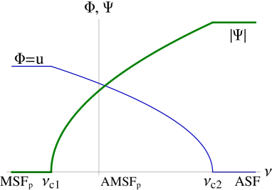
Figure 7: (Color online) Schematic atomic (thick) and molecular (thin) order parameters versus the FR detuning $\nu$ for the polar phase, with $\nu_{\rm c1}=\nu_{\rm c}^{\rm MSF_{\rm p}-AMSF_{\rm p}}$ and $\nu_{\rm c2}=\nu_{\rm c}^{\rm AMSF_{\rm p}-ASF}$.

IV.4.1 Polar AMSF: AMSF_p

A straightforward minimization of $f_{\rm amsf}[u,v]$, Eq.(LABEL:famsf) for $g_{2}<0$ leads to the AMSF_p phase, characterized by order parameters,

$$u_{p} =\sqrt{\frac{\lambda\mu_{m}-\tilde{g}_{am}\mu}{\lambda(g_{1}+g_{2})-\tilde{g}^{2}_{am}}},\ \ \ v_{p}=0,$$ (49a)

$$|\Psi_{-,p}| =\sqrt{\frac{(g_{1}+g_{2})\mu-\tilde{g}_{am}\mu_{m}}{\lambda(g_{1}+g_{2})-\tilde{g}_{am}^{2}}},$$ (49b)

where $\tilde{g}_{am}=g_{am}-m\alpha^{2}/2$.

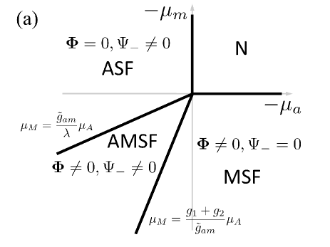
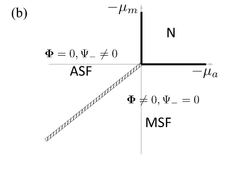
Figure 8: Mean-field phase diagrams for polar phase as a function of atomic and molecular chemical potentials, $\mu_{a}$, $\mu_{m}$, respectively. The ferromagnetic phase is similar but with different parameters. (a) For $\lambda(g_{1}+g_{2})-{\tilde{g}_{am}}^{2}>0$, all three superfluid phases—ASF, AMSF, and MSF—appear and are separated by continuous phase transitions (thick black lines). (b) For $\lambda(g_{1}+g_{2})-{\tilde{g}_{am}}^{2}<0$, AMSF is unstable, and the ASF and MSF are separated by a first-order transition (hatched double line).

The phase boundaries corresponding to the MSF_p - AMSF_p and AMSF_p - ASF transitions are also easily worked out (set by the vanishing of the atomic and molecular condensates, respectively) and are given by

$$\nu_{\rm c}^{\rm MSF_{p}-AMSF_{p}} =-\left(g_{1}+g_{2}-2\tilde{g}_{am}\right)n_{m},$$ (50a)

$$\approx-\frac{1}{2}\left(g_{1}+g_{2}-2\tilde{g}_{am}\right)n,$$ (50b)

$$\nu_{\rm c}^{\rm AMSF_{p}-ASF} =\left(2\lambda-\tilde{g}_{am}\right)n_{a},$$ (50c)

$$\approx\left(2\lambda-\tilde{g}_{am}\right)n,$$ (50d)

where we used $\mu_{m}=2\mu-\nu=(g_{1}+g_{2})n_{m}$ and $\mu=\lambda n_{a}$ to eliminate the molecular and atomic chemical potentials in favor of the molecular condensate $n_{m}$, the atomic condensate $n_{a}$, and the detuning $\nu$. We also used the fact that at low temperature and for weak interactions, $n_{m}\approx n/2$ and $n_{a}\approx n$ in the MSF and ASF, respectively.

It is clear from Fig. 8 (a) and Eq.(49b) for $\Psi_{-,p}$ that the condition

$$\lambda(g_{1}+g_{2})-\tilde{g}_{am}^{2}>0$$ (51)

is necessary for the stability of AMSF_p. We observe that in addition to setting the value of the finite momentum, $Q_{0}$ of the atomic condensate, the $p$-wave FR coupling, $\alpha$, expands the stability of the AMSF phase. Within the mean-field approximation, the MSF_p-AMSF_p and AMSF_p-ASF transitions are of second order. This will be qualitatively modified, as we see when we discuss fluctuation effects in Sec.VI.

For $\lambda(g_{1}+g_{2})-\tilde{g}_{am}^{2}<0$ [Fig. 8 (b)], the AMSF_p state is unstable, replaced by a direct first-order ASF-MSF_p transition. The corresponding phase boundary is given by the degeneracy condition of the ASF and MSF_p free energies

$$f_{\rm asf}=-\frac{\mu^{2}}{2\lambda}=-\frac{\mu_{m}^{2}}{2(g_{1}+g_{2})}=f_{\rm msf_{\rm p}}.$$ (52)

IV.4.2 Ferromagnetic AMSF: AMSF_fm

A minimization of the free energy, $f_{\rm amsf}[u,v]$ for a range of couplings shows that for intermediate detuning, the low-temperature state is the ferromagnetic AMSF_fm, characterized by

$$u_{fm} =\sqrt{\frac{2\lambda g_{2}\mu_{m}-g_{am}^{2}\mu_{m}-(g_{1}+g_{2})\tilde{g}_{am}\mu+(g_{1}-g_{2})g_{am}\mu+g_{am}\tilde{g}_{am}\mu_{m}}{4\lambda g_{1}g_{2}-4g_{2}g_{am}\tilde{g}_{am}-(g_{1}+g_{2})(m\alpha^{2}/2)^{2}}},\quad\quad\quad\quad$$ (53a)

$$v_{fm} =\sqrt{\frac{2\lambda g_{2}\mu_{m}-{\tilde{g}_{am}}^{2}\mu_{m}-(g_{1}+g_{2})g_{am}\mu+(g_{1}-g_{2})\tilde{g}_{am}\mu+g_{am}\tilde{g}_{am}\mu_{m}}{4\lambda g_{1}g_{2}-4g_{2}g_{am}\tilde{g}_{am}-(g_{1}+g_{2})(m\alpha^{2}/2)^{2}}},\quad\quad\quad\quad$$ (53b)

$$|\Psi_{fm}| =\sqrt{\frac{g_{2}(4g_{1}\mu-4g_{am}\mu_{m}+m\alpha^{2}\mu_{m})}{4\lambda g_{1}g_{2}-4g_{2}g_{am}\tilde{g}_{am}-(g_{1}+g_{2})(m\alpha^{2}/2)^{2}}}.$$ (53c)

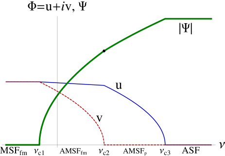
Figure 9: (Color online) Schematic atomic (thick) and molecular (thin and dashed) order parameters versus the FR detuning $\nu$ for ferromagnetic phases. The AMSF_fm-AMSF_p phase transition at $\nu_{c2}$ leads to kinks (change in slope) in the molecular ($u$) and atomic ($\Psi$) order parameter, later indicated by a black dot. Without loss of generality we choose the $\hat{n}$ axis (component of $u$) to lie along ${\textbf{\em Q}}_{0}$. The critical detunings are denoted by $\nu_{\rm c1}=\nu_{\rm c}^{\rm MSF_{\rm fm}-AMSF_{\rm fm}}$, $\nu_{\rm c2}=\nu_{\rm c}^{\rm AMSF_{\rm fm}-AMSF_{\rm p}}$, and $\nu_{\rm c3}=\nu_{\rm c}^{\rm AMSF_{\rm p}-ASF}$.

The behavior of these order parameters as a function of detuning, $\nu$, is illustrated in Fig. 9. With increasing detuning, the component $v$ (being smaller than $u$) vanishes first, signaling a transition of the ferromagnetic AMSF_fm to the polar AMSF_p state. Depending on the value of other parameters, upon further increase of $\nu$ the system either continuously transitions at $\nu_{\rm c}^{\rm AMSF_{p}-ASF}$ to one of the three ASF states or undergoes a first-order AMSF_fm-ASF transition with $u$ discontinuously jumping to zero when $v$ vanishes. As we discuss in Sec.V, on general grounds, beyond the mean-field approximation, we expect the transitions from such smectic like superfluid phases (AMSF_p,fm) to homogeneous and isotropic ASF states to be driven first-order by fluctuations.

The detuning phase boundaries corresponding to the MSF_fm - AMSF_fm and the AMSF_fm - AMSF_p transitions, determined by a vanishing of the atomic and the $v$ (transverse to ${\textbf{\em Q}}_{0}$) component of the molecular condensates, respectively, are given by

$$\nu_{\rm c}^{\rm MSF_{\rm fm}-AMSF_{\rm fm}} =-\left(g_{1}-2g_{am}+m\alpha^{2}/2\right)n_{m},$$ (54a)

$$\approx-\frac{1}{2}\left(g_{1}-2g_{am}+m\alpha^{2}/2\right)n,$$ (54b)

$$\nu_{\rm c}^{\rm AMSF_{\rm fm}-AMSF_{\rm p}} =\frac{8\lambda g_{2}+g_{am}\left(2m\alpha^{2}-4g_{2}\right)-m\alpha^{2}\left(g_{1}-g_{2}+m\alpha^{2}\right)}{4g_{2}+2m\alpha^{2}}n_{a}.$$ (54c)

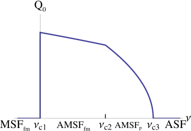
Figure 10: (Color online) Schematic detuning dependence of the momentum ${\textbf{\em Q}}_{0}$ of the atomic condensate starting with the MSF_fm, with $\nu_{\rm c1}=\nu_{\rm c}^{\rm MSF_{\rm fm}-AMSF_{\rm fm}}$, $\nu_{\rm c2}=\nu_{\rm c}^{\rm AMSF_{\rm fm}-AMSF_{\rm p}}$, and $\nu_{\rm c3}=\nu_{\rm c}^{\rm AMSF_{\rm p}-ASF}$.

As with the polar state, the stability of the AMSF_fm is dictated by a condition on the interaction couplings, given by

$$4\lambda g_{1}g_{2}-4g_{2}g_{am}\tilde{g}_{am}-(g_{1}+g_{2})(m\alpha^{2}/2)^{2}>0.$$ (55)

In the opposite regime of $4\lambda g_{1}g_{2}-4g_{2}g_{am}\tilde{g}_{am}-(g_{1}+g_{2})(m\alpha^{2}/2)^{2}<0$ [Fig. 8 (b)], the AMSF_fm state is unstable, replaced by a direct first-order MSF_fm-ASF transition. The corresponding phase boundary is given by the degeneracy condition of the ASF and MSF_fm free energies,

$$f_{\rm asf}=-\frac{\mu^{2}}{2\lambda}=-\frac{\mu_{m}^{2}}{g_{1}}=f_{\rm msf_{\rm fm}}.$$ (56)

IV.4.3 Renormalized molecular interactions couplings

We conclude this section by noting that near a FR the microscopic pseudopotentials $g_{i},\lambda_{i}$ are modified by quantum fluctuations, replaced by corresponding experimentally determined scattering lengths. To lowest order (Born approximation, valid at low densities) in the FR coupling $\alpha$, the diagrammatic corrections illustrated in Figs. 11 and Fig. 12 are given by

Figure 11: A lowest-order diagrammatic correction to molecular interaction coupling $g_{i}$.

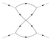
Figure 12: Next-lowest-order diagrammatic corrections to molecular interaction couplings $g_{i}$.

$$\delta g^{R}_{1} =\frac{m^{4}\alpha^{4}\Lambda^{2}}{\pi^{4}}\left(-\frac{2\pi^{2}}{15m\Lambda}+\frac{a_{bg}}{9\pi}-\frac{m\alpha^{2}}{16}(0.468)\right),$$ (57a)

$$\delta g^{R}_{2} =\frac{m^{4}\alpha^{4}\Lambda^{2}}{\pi^{4}}\left(-\frac{\pi^{2}}{15m\Lambda}-\frac{m\alpha^{2}}{16}(0.0489)\right),$$ (57b)

where $a_{bg}=a_{1}+a_{2}+2a_{12}$, the scattering lengths are defined by a standard relation, $\lambda_{\sigma\sigma^{\prime}}=\frac{4\pi\hbar^{2}a_{\sigma\sigma^{\prime}}}{m}$, and $\Lambda\approx 2\pi/d$ is the ultraviolet cutoff set by the interatomic potential range. In the large $\Lambda$ limit, $\delta g^{R}_{i}$ reduce to

$$\delta g^{R}_{1} \simeq\frac{m^{4}\alpha^{4}\Lambda^{2}}{\pi^{4}}\left(\frac{a_{bg}}{9\pi}-\frac{m\alpha^{2}}{16}(0.468)\right),$$ (58a)

$$\delta g^{R}_{2} \simeq-\frac{m^{5}\alpha^{6}\Lambda^{2}}{(2\pi)^{4}}(0.0489).$$ (58b)

This two-loop approximation (though valid only in the narrow FR limit), which finds $\delta g^{R}_{2}<0$, suggests that in the broad-resonance limit it is the MSF_p that prevails.

More generally, the importance of these fluctuation corrections to molecular interactions is that they provide a mechanism to tune and, in principle, even change the sign of the effective $g_{2}$, thereby allowing a detuning-driven MSF_p-MSF_fm transition.

V Elementary excitations

Having established the existence of a variety of superfluid ground states, we now turn our attention to the nature of low-energy excitations in each of these phases. As long as fluctuations remain finite for a range of a system’s parameters, the phases detailed in the previous section are self-consistently guaranteed to be stable in these regimes and to retain their qualitative form.

We study quantum fluctuations within each of the ASF, MSF and AMSF classes of phases established above. To this end we expand the atomic and molecular bosonic operators around their mean-field condensate values $\Psi_{\sigma}$, $\bm{\Phi}$,

$$\psi_{\sigma} = \Psi_{\sigma}+\delta\psi_{\sigma},$$ (59a)

$$\phi_{i} = \Phi_{i}+\delta\phi_{i},$$ (59b)

where $\delta\psi_{\sigma}$ ($\sigma=1,2$) are fluctuation fields for atoms of flavors $1$ and $2$, respectively, and $\delta\phi_{i}$ ($i=x,y,z$) are triplet of the $\ell=1$ molecular fluctuation fields.

For some of the analysis it is convenient to work in momentum space,

$$\delta\psi_{\sigma} = \frac{1}{\sqrt{V}}\sum_{{\textbf{\em k}}}a_{\sigma,{\textbf{\em k}}}\ e^{i{\textbf{\em k}}\cdot{\textbf{\em r}}},$$ (60a)

$$\delta\phi_{i} = \frac{1}{\sqrt{V}}\sum_{\textbf{\em k}}b_{i,{\textbf{\em k}}}\ e^{i{\textbf{\em k}}\cdot{\textbf{\em r}}}.$$ (60b)

Using the above momentum representation inside the Hamiltonian [Eq. (II)] and expanding to second order in the fluctuations operators $a_{\sigma,{\textbf{\em k}}}$, $b_{i,{\textbf{\em k}}}$, we obtain $H=H_{\text{mft}}[\Psi_{\sigma},\bm{\Phi}]+H_{f}$, with

$$H_{f}= \sum_{{\textbf{\em k}}}\Bigg{[}\sum_{\sigma=1,2}\left(\frac{1}{2}\tilde{\varepsilon}_{\sigma,{\textbf{\em k}}+{\textbf{\em Q}}_{\sigma}}a^{\dagger}_{\sigma,{\textbf{\em k}}+{\textbf{\em Q}}_{\sigma}}a_{\sigma,{\textbf{\em k}}+{\textbf{\em Q}}_{\sigma}}+\tilde{\lambda}_{\sigma}a_{\sigma,-{\textbf{\em k}}+{\textbf{\em Q}}_{\sigma}}a_{\sigma,{\textbf{\em k}}+{\textbf{\em Q}}_{\sigma}}\right)+t_{1}a^{{\dagger}}_{1,{\textbf{\em k}}+{\textbf{\em Q}}}a_{2,{\textbf{\em k}}-{\textbf{\em Q}}}+t_{2,{\textbf{\em k}}+{\textbf{\em Q}}}a_{1,{\textbf{\em k}}+{\textbf{\em Q}}}a_{2,-{\textbf{\em k}}-{\textbf{\em Q}}}$$

$$+\sum_{i=x,y,z}\left(\frac{1}{2}\tilde{\omega}_{i,{\textbf{\em k}}}b^{\dagger}_{i,{\textbf{\em k}}}b_{i,{\textbf{\em k}}}+\delta_{i}b_{i,-{\textbf{\em k}}}b_{i,{\textbf{\em k}}}\right)+\frac{1}{2}\sum_{\genfrac{}{}{0.0pt}{3}{i,j=x,y,z}{i\neq j}}\left(g_{ij}b^{{\dagger}}_{j,{\textbf{\em k}}}b_{i,{\textbf{\em k}}}+\gamma_{ij}b_{i,-{\textbf{\em k}}}b_{j,{\textbf{\em k}}}\right)$$

$$-\sum_{\sigma}\bm{\alpha}_{\overline{\sigma},{\textbf{\em k}}}\cdot{\bf b}^{\dagger}_{{\textbf{\em k}}}a_{\sigma,{\textbf{\em k}}+{\textbf{\em Q}}_{\sigma}}+h.c.\Bigg{]},$$ (61a)

$$\equiv\sum_{{\textbf{\em k}},\alpha,\beta}c^{\dagger}_{\alpha,{\textbf{\em k}}}\tilde{h}_{\textbf{\em k}}^{\alpha\beta}c_{\beta,{\textbf{\em k}}}$$ (61b)

where $\tilde{h}_{\textbf{\em k}}^{\alpha\beta}$ is a Bogoliubov Hamiltonian matrix defined by matrix elements

$$\tilde{\varepsilon}_{\sigma,{\bf k}} =\epsilon_{\bf k}-\mu_{\sigma}+2\lambda_{\sigma}|\Psi_{\sigma}|^{2}+\lambda_{12}|\Psi_{\overline{\sigma}}|^{2}+g_{am}|\bm{\Phi}|^{2},$$ (62a)

$$\tilde{\omega}_{i,{\bf k}} =\frac{1}{2}\epsilon_{\bf k}-\mu_{m}+g_{1}|\bm{\Phi}|^{2}+(g_{1}+2g_{2})|\Phi_{i}|^{2},$$

$$+g_{am}(|\Psi_{1}|^{2}+|\Psi_{2}|^{2}),$$ (62b)

$$\tilde{\lambda}_{\sigma} =\frac{1}{2}\lambda_{\sigma}\Psi^{*2}_{\sigma},$$ (62c)

$$t_{1} =\lambda_{12}\Psi_{1}\Psi^{*}_{2},$$ (62d)

$$t_{2,{\textbf{\em k}}} =\lambda_{12}\Psi_{1}^{*}\Psi_{2}^{*}-\alpha\bm{\Phi}^{*}\cdot{\textbf{\em k}},$$ (62e)

$$\delta_{i} =\frac{1}{2}g_{1}\Phi^{*}_{i}\Phi^{*}_{i}+\frac{1}{2}g_{2}\bm{\Phi}^{*}\cdot\bm{\Phi}^{*},$$ (62f)

$$g_{ij} =g_{1}\Phi^{*}_{i}\Phi_{j}+2g_{2}\Phi^{*}_{i}\Phi_{j},$$ (62g)

$$\gamma_{ij} =\frac{1}{2}g_{1}\Phi^{*}_{i}\Phi^{*}_{j},$$ (62h)

$$\bm{\alpha}_{\sigma=(1,2),{\textbf{\em k}}} =\pm\alpha\Psi_{\sigma,{\textbf{\em Q}}_{\sigma}}({\textbf{\em Q}}_{\sigma}-{\textbf{\em k}}/2),$$ (62i)

$\epsilon_{\bf k}=\frac{k^{2}}{2m}$, $\overline{1}=2,\overline{2}=1$, and we suppressed the Q subscript on the atomic condensate order parameter, $\Psi_{\sigma,{\textbf{\em Q}}}$. The ten-dimensional bosonic Nambu spinor $c_{\alpha,{\textbf{\em k}}}$ is given by

$$c_{\alpha,{\textbf{\em k}}}\equiv\left(a_{\sigma,{\textbf{\em k}}+{\textbf{\em Q}}_{\sigma}},b_{i,{\textbf{\em k}}},a^{\dagger}_{\sigma,-{\textbf{\em k}}+{\textbf{\em Q}}_{\sigma}},b^{\dagger}_{i,-{\textbf{\em k}}}\right).$$ (63)

A diagonalization of this ten-dimensional Bogoliubov Hamiltonian, preserving bosonic commutation relations of the $c_{\alpha,{\textbf{\em k}}}$ components gives the spectrum of the five modes throughout the phase diagram. This can be done numerically, but is not very enlightening. Instead, we study the problem one phase at a time, which allows a significantly more revealing solution of the problem.

V.1 ASF phases

In the simplest limit of a large positive detuning, $\nu>\nu^{\rm AMSF-ASF}$, the molecules are gapped, one or both species of the atoms are condensed at zero momentum, ${\textbf{\em Q}}=0$, and the system is in the ASF phases. As discussed in Sec. III, these are conventional well-studied superfluids, characterized by one Bogoliubov mode for each of the atomic $U(1)$ symmetry that is broken. In the ASF phases $\bm{\Phi}=0$, the three molecular modes are gapped and can therefore be integrated out (adiabatically eliminated). Away from the transition, this leads to only a small renormalization (that we will neglect) of effective parameters in the resulting $H_{f}$. From Eq. (61a) the atomic sector of the Bogoliubov Hamiltonian is then given by

$$H^{\rm ASF_{\sigma}}_{f}= \sum_{{\textbf{\em k}}}\left[\sum_{\sigma=1,2}\left(\frac{1}{2}\tilde{\varepsilon}_{\sigma,{\textbf{\em k}}}a^{\dagger}_{\sigma,{\textbf{\em k}}}a_{\sigma,{\textbf{\em k}}}+\tilde{\lambda}_{\sigma}a_{\sigma,-{\textbf{\em k}}}a_{\sigma,{\textbf{\em k}}}\right)+t_{1}a^{{\dagger}}_{\sigma,{\textbf{\em k}}}a_{\overline{\sigma},{\textbf{\em k}}}+t_{2,{\textbf{\em k}}}a_{\sigma,-{\textbf{\em k}}}a_{\overline{\sigma},{\textbf{\em k}}}\right]+h.c..$$ (64)

V.1.1 ASF_σ: single atomic species BEC

In the regime where only a single atomic species of $\psi_{1,2}$ condenses (i.e., $\Psi_{\sigma}\neq 0,\Psi_{\overline{\sigma}}=0$), the system is in an ASF_σ phase. Standard analysis then leads to a conventional, gapless atomic Bogoliubov sound mode for species $\sigma$

$$E^{(a)}_{k\sigma} = \sqrt{\frac{k^{2}}{2m}\Big{(}\frac{k^{2}}{2m}+\lambda_{\sigma}n\Big{)}},$$ (65a)

$$\approx c_{a}k,$$ (65b)

with $c_{a}\approx\sqrt{\frac{\lambda_{\sigma}n}{2m}}$, and a gapped atomic mode for the complementary atomic species $\overline{\sigma}$:

$$E^{(a)}_{k\overline{\sigma}} \simeq \frac{k^{2}}{2m^{*}_{-}}-\mu_{\overline{\sigma}}+\lambda_{12}\frac{n}{2}$$ (66)

where $\frac{n}{2}\simeq n_{1}=n_{2}$ for a balanced case. Above, the coupling parameters are those from Eq. (20), with $\bm{\Phi}=\Psi_{\overline{\sigma}}=0$, and $m^{*}_{\pm}$ are effective atomic masses renormalized by interaction

$$\frac{1}{m^{*}_{+}} = \frac{1}{m}+\frac{3n\alpha^{2}}{2(\nu-\lambda n+\frac{g_{am}}{2}n)},$$ (67a)

$$\frac{1}{m^{*}_{-}} = \frac{1}{m}-\frac{3n\alpha^{2}}{4(\nu-\lambda n+\frac{g_{am}}{2}n)}.\hskip 28.45274pt$$ (67b)

The remaining three molecular-like modes (corrected by coupling to atoms) are gapped and in a $k\rightarrow 0$ limit are given by

$$E^{(m)}_{k1} = E^{(m)}_{k2}=\frac{k^{2}}{4m}+\nu-\frac{\lambda_{\sigma}}{2}n+\frac{g_{am}}{2}n-\mu_{\overline{\sigma}},\quad\quad\quad$$ (68a)

$$E^{(m)}_{k3} \simeq \frac{k^{2}}{4m^{*}_{+}}+\nu-\frac{\lambda_{\sigma}}{2}n+\frac{g_{am}}{2}n-\mu_{\overline{\sigma}}.$$ (68b)

Figure 13: Schematic ASF single BEC (ASF_σ) excitation spectrum. The lowest curve is the atomic Bogoliubov mode and the upper curves are gapped atomic (thin) and molecular (thick) modes.

V.1.2 ASF₁₂: double atomic species BEC

In the regime where both atomic species of $\psi_{1,2}$ condense, that is, $\Psi_{1,2}\neq 0$, the system is in a two-species ASF₁₂ phase. Standard analysis, consistent with two $U(1)$ symmetries spontaneously broken, then leads to two gapless atomic Bogoliubov sound modes for species $1$ and $2$. Together with the gapped molecular excitations this leads to spectra of the five modes:

$$E^{(a_{12})}_{k1} = \sqrt{\frac{k^{2}}{2m}\Big{(}\frac{k^{2}}{2m}+2\lambda n\Big{)}},$$ (69a)

$$E^{(a_{12})}_{k2} \simeq c^{(a_{12})}k,$$ (69b)

$$E^{(m_{12})}_{k1} = E^{(m_{12})}_{k2}=\frac{k^{2}}{4m}+\nu-2\lambda n+g_{am}n,\quad\quad\,$$ (69c)

$$E^{(m_{12})}_{k3} \simeq \frac{k^{2}}{4m^{*}}+\nu-2\lambda n+g_{am}n,$$ (69d)

where for $E^{(a_{12})}_{k2}$ and $E^{(m_{12})}_{k3}$ we took $k\rightarrow 0$ and $\alpha\rightarrow 0$ limit and defined the sound velocity and effective atomic mass:

$$c^{(a_{12})} = \sqrt{\frac{(\lambda-\lambda_{12})n}{m}}-\frac{3n\alpha^{2}\sqrt{(\lambda-\lambda_{12})mn}}{4(\nu-2\lambda n+g_{am}n)},\quad\quad\quad$$ (70a)

$$\frac{1}{m^{*}} = \frac{1}{m}+\frac{3(\nu-(\lambda+\lambda_{12})n+g_{am}n)n\alpha^{2}}{(\nu-2\lambda n+g_{am}n)^{2}}.\quad\quad$$ (70b)

$E^{(a_{12})}_{k1}$ and $E^{(a_{12})}_{k2}$ are atomlike, gapless, in-phase and out-of-phase modes, respectively. $E^{(a_{12})}_{k2}$ and $E^{(m_{12})}_{k3}$ are modified by the FR interaction between atoms and molecules. The ASF-AMSF phase boundary is determined by the point where the molecular gap

$$E^{\rm ASF}_{\rm gap}=\nu-2\lambda n+g_{am}n$$ (71)

closes, and is consistent with the critical detuning determined by the development of the molecular order parameter that we found in Sec. IV.

Figure 14: Schematic ASF double BEC (ASF₁₂) excitation spectrum. There are two gapless atomic Bogoliubov modes (thin) as well as three gapped molecular modes (thick).

V.2 MSF phases

In the opposite limit of a large negative detuning, $\nu<\nu^{\rm MSF-AMSF}$ both atomic species are gapped, $\Psi_{\sigma}=0$, and $p$-wave molecules are condensed into one of the two ($\ell=1$) $\ell_{z}=0$ MSF_p and $\ell_{z}=\pm 1$ MSF_fm, isomorphic to spinor-1 condensates with well-studied properties ho.spinor.98 ; ho.yip.00 ; demler.zhou.02 . To see this, we note that the atomic Bogoliubov excitations are gapped and can therefore be integrated out. Away from the transition, they lead to only a small renormalization of effective parameters. Neglecting these small effects, the vanishing of $\bm{\alpha}_{\sigma,{\textbf{\em k}}}=\pm\alpha\Psi_{\sigma,{\textbf{\em Q}}_{\sigma}}({\textbf{\em Q}}_{\sigma}-{\textbf{\em k}}/2)=0$ decouples the Hamiltonian, $H_{f}=H_{a}+H_{m}$ into atomic and molecular parts, that then are straightforwardly diagonalized.

The atomic sector, $H_{a}$ is of standard Bogoliubov form, simplified to a $2\times 2$ form by $t_{1}=\tilde{\lambda}_{\sigma}=0$ inside the MSF phases, leading to the atomic excitation spectrum, that for the symmetric case of $\mu_{1}=\mu_{2}\equiv\mu$ is given by

$$E^{\rm MSF}_{a,{\textbf{\em k}}}=\sqrt{(\tilde{\varepsilon}_{{\textbf{\em k}}}+|\alpha\bm{\Phi}\cdot{\textbf{\em k}}|)(\tilde{\varepsilon}_{{\textbf{\em k}}}-|\alpha\bm{\Phi}\cdot{\textbf{\em k}}|)},$$ (72)

where $\tilde{\varepsilon}_{{\textbf{\em k}}}=k^{2}/2m-\mu+g_{am}|\bm{\Phi}|^{2}$.

One key observation is that already inside the MSF phases the atomic spectrum, $E^{\rm MSF}_{a,{\textbf{\em k}}}$ (degenerate for $\sigma=1,2$ species) develops a minimum at a nonzero momentum ${\textbf{\em k}}_{\rm min}={\textbf{\em Q}}_{\rm p,fm}$, with the corresponding atomic gap minimum, $E^{\rm MSF_{p,fm}}_{a,{\rm gap}}$, given by a value dependent on the nature of the MSF_p,fm phase.

V.2.1 MSF_p state : $g_{2}<0$

As analyzed in Sec. IV, the MSF_p phase is defined by a molecular condensate order parameter, which can be taken to be a three-dimensional real vector, $\bm{\Phi}=\bm{u}=\Phi_{\rm p}\hat{\bm{n}}$, with $n_{m}=|\Phi_{\rm p}|^{2}$. In terms of the molecular condensate density $n_{m}\approx n/2$ the atomic chemical potential for the symmetric case, $\mu_{1}=\mu_{2}=\mu$ is given by

$$\mu=\frac{1}{2}(\mu_{m}+\nu)=\frac{1}{2}\left((g_{1}+g_{2})n_{m}+\nu\right),$$ (73)

controlled by the FR detuning, $\nu$.

For this symmetric case $\mu_{1}=\mu_{2}=\mu$ (easily generalizable for the asymmetric, imbalanced case), the atomic spectrum minimum is characterized by

$$k_{\rm min} = Q_{\rm p},$$ (74a)

$$= \alpha m\sqrt{n_{m}},$$

$$E^{\rm(MSF_{p},a)}_{\rm gap} = -\mu+g_{am}n_{m}-\frac{m\alpha^{2}n_{m}}{2},\quad\quad$$ (74b)

where in an isotropic trap the orientation of ${\textbf{\em k}}_{\rm min}$ is spontaneously chosen. The MSF_p-AMSF_p phase transition boundary is set by the closing of this atomic gap and is given by

$$\nu^{\rm MSF_{p}-AMSF_{p}}_{c}=-\left(g_{1}+g_{2}-2g_{am}+m\alpha^{2}\right)n_{m}.$$ (75)

Reassuringly, this is identical to the critical detuning for this phase boundary, which we obtained in Sec. IV from the value of detuning at which the finite-momentum atomic order-parameter became nonzero.

The diagonalization of molecular part $H_{m}$ is also straightforward, and is identical to the case of the spinor-1 condensates ho.spinor.98 ; ho.yip.00 ; demler.zhou.02 , with effective parameters of our physically distinct, $p$-wave resonant scalar Bose gas. Substituting characteristics of the polar phase MSF_p (order parameters, $\mu$, $\mu_{m}\approx(g_{1}+g_{2})n_{m}$, $g_{2}<0$, etc. from above) into $H_{m}$, we obtain

$$H^{\rm MSF_{p}}_{m}= \sum_{\textbf{\em k}}\Bigg{[}\left(\frac{1}{2}\epsilon_{{\textbf{\em k}}}+(g_{1}+g_{2})n_{m}\right)b^{{\dagger}}_{\parallel,{\textbf{\em k}}}b_{\parallel,{\textbf{\em k}}}$$

$$+\bigg{(}\frac{1}{2}\epsilon_{{\textbf{\em k}}}+|g_{2}|n_{m}\bigg{)}{\bf b}^{{\dagger}}_{\perp,{\textbf{\em k}}}\cdot{\bf b}_{\perp,{\textbf{\em k}}}$$

$$+\Bigg{(}\frac{1}{2}(g_{1}+g_{2})n_{m}b_{\parallel,-{\textbf{\em k}}}b_{\parallel,{\textbf{\em k}}}$$

$$+\frac{1}{2}g_{2}n_{m}{\bf b}_{\perp,-{\textbf{\em k}}}\cdot{\bf b}_{\perp,{\textbf{\em k}}}+h.c.\Bigg{)}\Bigg{]},$$ (76)

where ${\bf b}_{\perp,{\textbf{\em k}}}$ are two degenerate transverse (to ${\textbf{\em Q}}_{\rm p}$) molecular modes. This leads to three Bogoliubov-type dispersions,

$$E^{\rm MSF_{p}}_{\parallel,k} = \frac{1}{2}\sqrt{\epsilon_{{\textbf{\em k}}}^{2}+4(g_{1}+g_{2})n_{m}\epsilon_{{\textbf{\em k}}}},$$ (77a)

$$\simeq \sqrt{\frac{(g_{1}+g_{2})n_{m}}{2m}}k,$$ (77b)

$$E^{\rm MSF_{p}}_{\perp,k} = \frac{1}{2}\sqrt{\epsilon_{{\textbf{\em k}}}^{2}+4|g_{2}|n_{m}\epsilon_{{\textbf{\em k}}}},$$ (77c)

$$\simeq \sqrt{\frac{|g_{2}|n_{m}}{2m}}k,$$ (77d)

where the longitudinal mode, $E^{\rm MSF_{p}}_{\parallel,k}$ describes the conventional MSF phase fluctuations and the doubly degenerate transverse mode, $E^{\rm MSF_{p}}_{\perp,k}$ is the dispersion for the $\ell=1$ molecular orientational spin-waves. From the second set of $k\rightarrow 0$ expressions we read off the corresponding phase and spin-wave velocities, given by

$$c^{\rm MSF_{p}}_{\parallel} = \sqrt{\frac{(g_{1}+g_{2})n_{m}}{2m}},$$ (78a)

$$c^{\rm MSF_{p}}_{\perp} = \sqrt{\frac{|g_{2}|n_{m}}{2m}}.$$ (78b)

Figure 15: Schematic excitation spectrum for the MSF_p. The doubly degenerate atomic spectrum (upper thin curve) exhibits a minimum gap at nonzero $k$, a precursor of finite-momentum atomic condensation inside the AMSF_p. The molecular spectra (thick curves), one longitudinal (lowest) and two degenerate transverse (middle) modes, are of Bogoliubov type.

V.2.2 MSF_fm state : $g_{2}>0$

Inside the MSF_fm state, the molecular condensate order parameter is given by $\bm{\Phi}=\frac{\Phi_{\rm fm}}{\sqrt{2}}(\hat{\bm{n}}+i\hat{\bm{m}})$, expressed in terms of an orthonormal triad, $\hat{\bm{n}}\times\hat{\bm{m}}=\hat{\bm{\ell}}$. From the earlier mean-field analysis, the molecular condensate density is given by $n_{m}=|\bm{\Phi}|^{2}=\mu_{m}/g_{1}$, leading for the symmetric case, $\mu_{1}=\mu_{2}=\mu$

$$\mu=\frac{1}{2}\left(g_{1}n_{m}+\nu\right).$$ (79)

To lowest order, the atomic spectrum inside MSF_fm has identical structure as that of the MSF_p state [Eq. (77)], but with the replacement $g_{1}+g_{2}\rightarrow g_{1}$ and $\alpha^{2}\rightarrow\alpha^{2}/2$,

$$k_{\rm min} = Q_{\rm fm},$$ (80a)

$$= \frac{1}{\sqrt{2}}\alpha m\sqrt{n_{m}},$$

$$E^{\rm(MSF_{fm},a)}_{\rm gap} = -\mu+g_{am}n_{m}-\frac{m\alpha^{2}n_{m}}{4}.\quad\quad$$ (80b)

The MSF_fm-AMSF_fm phase transition boundary is determined by the vanishing of the atomic gap, and is given by

$$\nu^{\rm MSF_{fm}-AMSF_{fm}}_{c}=-\left(g_{1}-2g_{am}+\frac{1}{2}m\alpha^{2}\right)n_{m},$$ (81)

identical to the critical detuning obtained from mean-field theory for the order parameter in Sec. IV.

Using the above parameters characteristic of the MSF_fm phase inside $H_{m}$, the molecular sector of the Hamiltonian reduces to

$$H^{\rm MSF_{fm}}_{m} = \sum_{\textbf{\em k}}\Big{[}(\frac{1}{2}\epsilon_{{\textbf{\em k}}}+2g_{2}n_{m})b^{{\dagger}}_{+,{\textbf{\em k}}}b_{+,{\textbf{\em k}}}+(\frac{1}{2}\epsilon_{{\textbf{\em k}}}+g_{1}n_{m})b^{{\dagger}}_{-,{\textbf{\em k}}}b_{-,{\textbf{\em k}}}+\frac{1}{2}\epsilon_{{\textbf{\em k}}}b^{{\dagger}}_{z,{\textbf{\em k}}}b_{z,{\textbf{\em k}}}+\frac{1}{2}g_{1}n_{m}b_{-,{\textbf{\em k}}}b_{-,{\textbf{\em k}}}+\frac{1}{2}g_{1}n_{m}b^{{\dagger}}_{-,{\textbf{\em k}}}b^{{\dagger}}_{-,{\textbf{\em k}}}\Big{]},$$

where

$$b_{+} = \frac{1}{\sqrt{2}}(b_{n}+ib_{m}),$$ (83a)

$$b_{-} = \frac{1}{\sqrt{2}}(b_{n}-ib_{m}),$$ (83b)

are expressed in terms of operators $b_{n}$, $b_{m}$, that are components of $\bf b$ along $\hat{\bm{n}}$, $\hat{\bm{m}}$, respectively. Diagonalization of the above Hamiltonian then gives the following spectrum

$$E^{\rm MSF_{fm}}_{z,k} = \frac{1}{2}\epsilon_{{\textbf{\em k}}}=\frac{k^{2}}{4m},$$ (84a)

$$E^{\rm MSF_{fm}}_{+,k} = \frac{1}{2}\epsilon_{{\textbf{\em k}}}+2g_{2}n_{m},$$ (84b)

$$E^{\rm MSF_{fm}}_{-,k} = \frac{1}{2}\sqrt{\epsilon_{{\textbf{\em k}}}^{2}+4g_{1}n_{m}\epsilon_{{\textbf{\em k}}}},$$ (84c)

$$\simeq \sqrt{\frac{g_{1}n_{m}}{2m}}k,$$ (84d)

where the Bogoliubov sound speed is given by $c_{\rm MSF_{fm}}=\sqrt{g_{1}n_{m}/2m}$.

We note that despite a three-dimensional coset space, $SO(3)$ characterizing MSF_fm, only two modes (linear and quadratic in $k$) exhibit a spectrum that vanishes in $k\rightarrow 0$ limit. The spectrum $E^{\rm MSF_{fm}}_{-,k}$ is that of a conventional Bogoliubov superfluid phase, here associated with the $U(1)$ broken gauge symmetry of the molecular condensate. The quadratic in $k$ gapless spectrum is that of the ferromagnetic spin waves, where the two components of the spinor are canonically conjugate and, as a result, combine into a single low-frequency mode.

Figure 16: Schematic excitation spectrum for the MSF_fm. The doubly degenerate atomic spectrum (thin curves) exhibits a minimum gap at nonzero $k$, a precursor of finite momentum atomic condensation. The molecular spectrum (thick curves) consists of a longitudinal gapless quadratic ferromagnetic spin-wave mode (lowest), a Bogoliubov sound mode, and a quadratic gapped mode.

V.3 AMSF phases

To obtain the spectrum inside the AMSF phases requires a solution of the fully general Hamiltonian, $H_{f}$ [Eq. (61a)]. Because in this superfluid state all atomic and molecular modes are coupled, a direct BdG analysis generically involves a diagonalization of a $10\times 10$ Bogoliubov matrix. This can be done numerically. However, instead, below we take a complementary coherent-state path-integral approach that allows us to obtain the modes and dispersions analytically, leading to more insight into their structure. Using the formulation of the problem introduced in Sec. II.0.2, we analyze the low-energy fluctuations in the AMSF states using the coherent-state Lagrangian density, ${\cal L}[\psi_{\sigma},\bm{\phi}]={\cal L}_{\rm MFT}[\Psi_{\sigma},\bm{\Phi}]+\delta{\cal L}$ [Eq. (18)], where ${\cal L}_{\rm MFT}[\Psi_{\sigma},\bm{\Phi}]$ is the mean-field Lagrangian defining the AMSF phase and $\delta{\cal L}$ is the Lagrangian density of the quadratic fluctuations. To obtain $\delta{\cal L}$ we expand the atomic and molecular bosonic fields $\psi_{\sigma},\bm{\phi}$ about their mean-field values (for clarity of notation in this section we choose to use $\rho$ instead of $n$ of the previous sections, where $\rho_{\sigma}=n_{a}/2$, $\rho_{m}=n_{m}$, and $\rho_{s}=n$),

$$\psi_{\sigma} = \sqrt{\rho_{\sigma}}e^{i\theta_{\sigma}+i{\textbf{\em Q}}_{\sigma}\cdot{\textbf{\em r}}},$$ (85a)

$$\bm{\phi} = \sqrt{\rho_{m}}\bm{\hat{\phi}}e^{i\varphi},$$ (85b)

where ${\textbf{\em Q}}_{\sigma}=\pm{\textbf{\em Q}}$ for $\sigma=1,2$, respectively, $\rho_{m}=\rho_{m0}+\delta\rho_{m}$ and $\rho_{\sigma}=\rho_{0}+\delta\rho_{\sigma}$ are the molecular and atomic densities, with the mean-field values $\rho_{m0}=|\bm{\Phi}|^{2}$ and $\rho_{0}=|\Psi_{\sigma}|^{2}$, and, based on Eq. (41), with the latter $\sigma$ independent in the AMSF phase. In addition to the density fluctuations, $\delta\rho_{m},\delta\rho_{\sigma}$, and two atomic and one molecular superfluid phases, $\theta_{\sigma}$, $\varphi$, the molecular Goldstone modes are characterized by a unit vector, $\bm{\hat{\phi}}$, whose form depends on the polar or ferromagnetic nature of the AMSF state:

$$\bm{\hat{\phi}} = {\hat{\bm{n}}},\ \ \ \mbox{for AMSF${}_{\rm p}$},$$

$$= \frac{1}{\sqrt{2}}({\hat{\bm{n}}}+i{\hat{\bm{m}}}),\ \ \ \mbox{for AMSF${}_{\rm fm}$}.$$

Substituting these parametrizations of the atomic and molecular fields into the Lagrangian, Eq. (19), we obtain $\delta{\cal L}$ that controls fluctuations in the AMSF phases.

V.3.1 AMSF_p

Focusing first on the polar state, with $\bm{\phi}=\sqrt{\rho_{m}}{\hat{\bm{n}}}e^{i\varphi}$, we find

$$\delta{\cal L}_{\rm p} = \rho_{\sigma}(i\partial_{\tau}\theta_{\sigma}-\mu_{\sigma})+\frac{\rho_{\sigma}}{2m}({\bm{\nabla}}\theta_{\sigma}+{\textbf{\em Q}}_{\sigma})^{2}+\rho_{m}(i\partial_{\tau}\varphi-\mu_{m})+\frac{\rho_{m}}{4m}({\bm{\nabla}}\varphi)^{2}+\frac{\rho_{m}}{4m}({\bm{\nabla}}\hat{\bm{n}})^{2}$$

$$- \alpha\sqrt{\rho_{m}\rho_{1}\rho_{2}}\;\hat{\bm{n}}\cdot({\bm{\nabla}}\theta_{1}-{\bm{\nabla}}\theta_{2}+2{\textbf{\em Q}})\cos(\varphi-\theta_{1}-\theta_{2})+\frac{1}{8m\rho_{\sigma}}({\bm{\nabla}}\rho_{\sigma})^{2}+\frac{1}{16m\rho_{m}}({\bm{\nabla}}\rho_{m})^{2}+\frac{\lambda_{\sigma}}{2}\rho_{\sigma}^{2}$$

$$+ \lambda_{12}\rho_{1}\rho_{2}+g_{am}(\rho_{1}+\rho_{2})\rho_{m}+\frac{g}{2}\rho_{m}^{2}-{\cal L}_{\rm MFT}[\rho_{0},\rho_{m0},\hat{\bm{n}}_{0},{\textbf{\em Q}}],$$

$$= i\delta\rho_{+}\partial_{\tau}\theta_{+}+\frac{\rho_{0}}{m}({\bm{\nabla}}\theta_{+})^{2}+i\delta\rho_{-}\partial_{\tau}\theta_{-}+\frac{\rho_{0}}{m}({\bm{\nabla}}\theta_{-}+{\textbf{\em Q}})^{2}+i\delta\rho_{m}\partial_{\tau}\varphi+\frac{\rho_{m0}}{4m}({\bm{\nabla}}\varphi)^{2}+\frac{\rho_{m0}}{4m}({\bm{\nabla}}\hat{\bm{n}})^{2}$$

$$- 2\alpha\rho_{0}\sqrt{\rho_{m0}}\;\hat{\bm{n}}\cdot({\bm{\nabla}}\theta_{-}+{\textbf{\em Q}})\cos(\varphi-2\theta_{+})$$

$$+ \frac{1}{16m\rho_{0}}({\bm{\nabla}}\rho_{+})^{2}+\frac{1}{16m\rho_{0}}({\bm{\nabla}}\rho_{-})^{2}+\frac{1}{16m\rho_{m0}}({\bm{\nabla}}\rho_{m})^{2}+\frac{\lambda}{4}\delta\rho_{+}^{2}+\frac{\lambda}{4}\delta\rho_{-}^{2}+\frac{\lambda_{12}}{4}(\delta\rho_{+}^{2}-\delta\rho_{-}^{2})+g_{am}\delta\rho_{+}\delta\rho_{m}+\frac{g}{2}\delta\rho_{m}^{2},$$

where $g\equiv g_{1}+g_{2}$, $\lambda=\lambda_{1}=\lambda_{2}$ for simplicity, and

$$\theta_{\pm} = \frac{1}{2}(\theta_{1}\pm\theta_{2}),$$ (88a)

$$\delta\rho_{\pm} = \delta\rho_{1}\pm\delta\rho_{2},$$ (88b)

$$\mu = \frac{1}{2}(\mu_{1}+\mu_{2}),$$ (88c)

$$h = \frac{1}{2}(\mu_{1}-\mu_{2}),$$ (88d)

Q $$= \alpha m\sqrt{\rho_{m0}}{\hat{\bm{n}}_{0}}.$$ (88e)

In the second form [Eq. (87)], we expanded the Lagrangian about its mean-field value ${\cal L}_{\rm MFT}$ to quadratic order in fluctuations, $\theta_{\sigma},\varphi,\delta\rho_{\sigma},\delta\rho_{m}$, and neglected the constant and subdominant contributions, that are negligible at long scales and low energies. We note that, as usual, the linear terms in $\delta{\cal L}_{\rm p}$ [Eq. (87)] vanish identically, enforced by the saddle-point equations for the condensates, $\rho_{-0}$, $\rho_{m0}$, and Q.

Examining the last form of $\delta{\cal L}_{\rm p}$, it is clear that important simplifications take place at long scales. In particular, the Feshbach resonant (Josephson-like) coupling, $-\alpha\cos(\varphi-2\theta_{+})$, between the closed-channel molecules and atoms (which is always relevant in three dimensions and therefore acts like a “mass”) locks their phases together at low energies giving

$$\varphi=2\theta_{+}.$$ (89)

Integrating $\varphi$ out and completing the square for the ${\bm{\nabla}}\theta_{-}+{\textbf{\em Q}}$ and $\hat{\bm{n}}$, to lowest order then gives

$$\delta{\cal L}_{\rm p} = i(\delta\rho_{+}+2\delta\rho_{m})\partial_{\tau}\theta_{+}+\frac{\rho_{s0}}{m}({\bm{\nabla}}\theta_{+})^{2}+i\delta\rho_{-}\partial_{\tau}\theta_{-}+\frac{\rho_{0}}{m}({\bm{\nabla}}\theta_{-}+{\textbf{\em Q}}-\alpha m\sqrt{\rho_{m0}}\hat{\bm{n}})^{2}+\frac{\rho_{m0}}{4m}({\bm{\nabla}}\hat{\bm{n}})^{2}$$

$$+ \frac{1}{16m\rho_{0}}({\bm{\nabla}}\rho_{+})^{2}+\frac{1}{16m\rho_{0}}({\bm{\nabla}}\rho_{-})^{2}+\frac{1}{16m\rho_{m0}}({\bm{\nabla}}\rho_{m})^{2}+\frac{\lambda}{4}\delta\rho_{+}^{2}+\frac{\lambda}{4}\delta\rho_{-}^{2}+\frac{\lambda_{12}}{4}(\delta\rho_{+}^{2}-\delta\rho_{-}^{2})+g_{am}\delta\rho_{+}\delta\rho_{m}+\frac{g}{2}\delta\rho_{m}^{2},$$

$$= i(\delta\rho_{+}+2\delta\rho_{m})\partial_{\tau}\theta_{+}+\frac{\rho_{s0}}{m}({\bm{\nabla}}\theta_{+})^{2}+i\delta\rho_{-}\partial_{\tau}\theta_{-}+\frac{\rho_{0}}{m}({\bm{\nabla}}\theta_{-}-\alpha m\sqrt{\rho_{m0}}\delta\hat{\bm{n}})^{2}+\frac{\rho_{m0}}{4m}({\bm{\nabla}}\hat{\bm{n}})^{2}$$

$$+ \frac{1}{16m\rho_{0}}({\bm{\nabla}}\rho_{+})^{2}+\frac{1}{16m\rho_{0}}({\bm{\nabla}}\rho_{-})^{2}+\frac{1}{16m\rho_{m0}}({\bm{\nabla}}\rho_{m})^{2}+\frac{\lambda}{4}\delta\rho_{+}^{2}+\frac{\lambda}{4}\delta\rho_{-}^{2}+\frac{\lambda_{12}}{4}(\delta\rho_{+}^{2}-\delta\rho_{-}^{2})+g_{am}\delta\rho_{+}\delta\rho_{m}+\frac{g}{2}\delta\rho_{m}^{2},$$

$$= i(\delta\rho_{+}+2\delta\rho_{m})\partial_{\tau}\theta_{+}+\frac{\rho_{s0}}{m}({\bm{\nabla}}\theta_{+})^{2}+i\delta\rho_{-}\partial_{\tau}\theta_{-}+\frac{\rho_{0}}{m}(\partial_{z}\theta_{-})^{2}+\frac{1}{4m^{3}\alpha^{2}}({\bm{\nabla}}{\bm{\nabla}}_{\perp}\theta_{-})^{2}$$

$$+ \frac{1}{16m\rho_{0}}({\bm{\nabla}}\rho_{+})^{2}+\frac{1}{16m\rho_{0}}({\bm{\nabla}}\rho_{-})^{2}+\frac{1}{16m\rho_{m0}}({\bm{\nabla}}\rho_{m})^{2}+\frac{\lambda}{4}\delta\rho_{+}^{2}+\frac{\lambda}{4}\delta\rho_{-}^{2}+\frac{\lambda_{12}}{4}(\delta\rho_{+}^{2}-\delta\rho_{-}^{2})+g_{am}\delta\rho_{+}\delta\rho_{m}+\frac{g}{2}\delta\rho_{m}^{2},$$

where

$$\rho_{s0} = \rho_{0}+\rho_{m0},$$ (91a)

$$\hat{\bm{z}} = \hat{\textbf{\em Q}},$$ (91b)

and in the second form [Eq. (90)] we used the minimum value of Q [Eq. (88e)] characterizing the AMSF_p phase, which leads to a minimal-like coupling between ${\bm{\nabla}}\theta_{-}$ and $\delta\hat{\bm{n}}$, the latter transverse ($\perp$) to $\hat{\bm{n}}_{0}$ and Q. Subsequently, to obtain our final expression, we integrated out $\delta\hat{\bm{n}}$ that to lowest order via a Higgs-like mechanism introduced a low-energy constraint

$$\delta\hat{\bm{n}} = \frac{1}{\alpha m\sqrt{\rho_{m0}}}{\bm{\nabla}}_{\perp}\theta_{-},$$ (92a)

$$= \frac{1}{Q}{\bm{\nabla}}_{\perp}\theta_{-}.$$ (92b)

Using it inside the $(\nabla\hat{\bm{n}})^{2}$ term then leads to a quantum smecticlike “elasticity” for the $\theta_{-}$ Goldstone mode, with $\hat{\bm{z}}$ chosen to lie along Q, that is, $\hat{\bm{z}}=\hat{{\textbf{\em Q}}}$. This smectic dispersion is expected based on the underlying rotational symmetry, which is spontaneously broken by the periodic AMSF_p state. It is closely related to other periodic superfluids, such as, for example, the Fulde-Ferrell-Larkin-Ovchinnikov pair-density wave states ff.64 ; lo.65 ; radzihovsky.vishwanath.08 ; FFLOlongLeo .

As a final step we now integrate out the densities $\delta\rho_{\pm}$ fluctuations, obtaining at long scales (where ${\bm{\nabla}}\rho_{\pm}$ can be neglected) our final form for the Goldstone mode Lagrangian in the AMSF_p state:

$$\delta{\cal L}_{\rm p} = \frac{1}{2}\chi_{+}(\partial_{\tau}\theta_{+})^{2}+\frac{\rho_{s0}}{m}({\bm{\nabla}}\theta_{+})^{2}+\frac{1}{2}\chi_{-}(\partial_{\tau}\theta_{-})^{2}+\frac{\rho_{0}}{m}(\partial_{z}\theta_{-})^{2}+\frac{1}{4m^{3}\alpha^{2}}({\bm{\nabla}}^{2}_{\perp}\theta_{-})^{2},$$ (93)

where the compressibilities are given by

$$\chi_{-} = \frac{2}{\lambda-\lambda_{12}},$$ (94a)

$$\chi_{+} = \frac{g+4g_{+}-4g_{am}}{g_{+}g-g_{am}^{2}},$$ (94b)

with $g_{+}=\frac{1}{2}(\lambda+\lambda_{12})$.

Thus, the in-phase and out-of-phase Goldstone modes are characterized by dispersions:

$$\omega_{+p}({\textbf{\em k}}) = c_{+}k,$$ (95a)

$$\omega_{-p}({\textbf{\em k}}) = \sqrt{(Bk_{z}^{2}+Kk_{\perp}^{4})/\chi_{-}},$$ (95b)

with defined parameters

$$c_{+} = \sqrt{\frac{2\rho_{s0}}{\chi_{+}m}},$$ (96a)

$$B = \frac{2\rho_{0}}{m},$$ (96b)

$$K = \frac{1}{2m^{3}\alpha^{2}}.$$ (96c)

The linear $\omega_{+}(k)$ dispersion of the superfluid phase $\theta_{+}$ is the expected Bogoliubov mode corresponding to the superfluid order. The anisotropic smecticlike dispersion of the “phonon” $\theta_{-}$ is a reflection of the uniaxial finite-momentum order in the AMSF_p state, akin to the FF superconductor ff.64 ; FFLOlongLeo .

Figure 17: (Color online) The diagram defining various vectors appearing in Eq. (97). $\vec{V}=\hat{\bm{n}}\cos(\varphi-2\theta_{+})-\hat{\bm{m}}\sin(\varphi-2\theta_{+})$, while $\varphi-2\theta_{+}$ is measured relative to the $\hat{\bm{n}}$ axis and $\varphi_{0}$ is measured relative to $\hat{\bm{z}}$.

V.3.2 AMSF_fm

The analysis for the AMSF_fm phase is very similar, with only a single modification of the MSF_fm order parameter, given instead by $\bm{\hat{\phi}}$ in Eq. (86). The corresponding fluctuations Lagrangian density is given by

$$\delta{\cal L}_{\rm fm} \approx i\delta\rho_{+}\partial_{\tau}\theta_{+}+\frac{\rho_{0}}{m}({\bm{\nabla}}\theta_{+})^{2}+i\delta\rho_{-}\partial_{\tau}\theta_{-}+\frac{\rho_{0}}{m}({\bm{\nabla}}\theta_{-}+{\textbf{\em Q}})^{2}+i\delta\rho_{m}\partial_{\tau}(\varphi-\varphi_{0})+i\rho_{m0}\hat{\bm{n}}\cdot\partial_{\tau}\hat{\bm{m}}+\frac{\rho_{m0}}{4m}({\bm{\nabla}}\varphi)^{2}$$

$$+ \frac{\rho_{m0}}{8m}({\bm{\nabla}}\hat{\bm{n}})^{2}+\frac{\rho_{m0}}{8m}({\bm{\nabla}}\hat{\bm{m}})^{2}+\frac{1}{16m\rho_{m0}}({\bm{\nabla}}\rho_{m})^{2}-\sqrt{2}\alpha\rho_{0}\sqrt{\rho_{m0}}\;({\bm{\nabla}}\theta_{-}+{\textbf{\em Q}})\cdot\left[\hat{\bm{n}}\cos(\varphi-2\theta_{+})-\hat{\bm{m}}\sin(\varphi-2\theta_{+})\right]$$

$$+ \frac{1}{16m\rho_{0}}({\bm{\nabla}}\rho_{+})^{2}+\frac{1}{16m\rho_{0}}({\bm{\nabla}}\rho_{-})^{2}+\frac{\lambda}{4}\delta\rho_{+}^{2}+\frac{\lambda}{4}\delta\rho_{-}^{2}+\frac{\lambda_{12}}{4}(\delta\rho_{+}^{2}-\delta\rho_{-}^{2})+g_{am}\delta\rho_{+}\delta\rho_{m}+\frac{g_{1}}{2}\delta\rho_{m}^{2},$$

$$\approx i(\delta\rho_{+}+2\delta\rho_{m})\partial_{\tau}\theta_{+}+\frac{\rho_{s0}}{m}({\bm{\nabla}}\theta_{+})^{2}+i\delta\rho_{-}\partial_{\tau}\theta_{-}+\frac{\rho_{0}}{m}\left({\bm{\nabla}}\theta_{-}-\frac{1}{\sqrt{2}}\alpha m\sqrt{\rho_{m0}}\delta\hat{\bm{n}}\right)^{2}+i\rho_{m0}\delta\hat{\bm{n}}\cdot\partial_{\tau}\hat{\bm{m}}$$

$$+ \frac{\rho_{m0}}{8m}({\bm{\nabla}}\hat{\bm{n}})^{2}+\frac{\rho_{m0}}{8m}({\bm{\nabla}}\hat{\bm{m}})^{2}+\frac{1}{16m\rho_{0}}({\bm{\nabla}}\rho_{+})^{2}+\frac{1}{16m\rho_{0}}({\bm{\nabla}}\rho_{-})^{2}+\frac{1}{16m\rho_{m0}}({\bm{\nabla}}\rho_{m})^{2}$$

$$+ \frac{\lambda}{4}\delta\rho_{+}^{2}+\frac{\lambda}{4}\delta\rho_{-}^{2}+\frac{\lambda_{12}}{4}(\delta\rho_{+}^{2}-\delta\rho_{-}^{2})+g_{am}\delta\rho_{+}\delta\rho_{m}+\frac{g_{1}}{2}\delta\rho_{m}^{2},$$ (97b)

where to get the second form we performed a gauge transformation to absorb the $\hat{\bm{n}}-\hat{\bm{m}}$ planar rotations angle $\hat{\bm{m}}\cdot\partial_{\tau}\hat{\bm{n}}\equiv\partial_{\tau}\varphi_{0}$ into $\partial_{\tau}\varphi$ and to simplify the FR term, as well as subsequently integrated out $\varphi$, completed the square into a minimal-like coupling for ${\bm{\nabla}}\theta_{-}$, and chose ${\textbf{\em Q}}=\alpha m\sqrt{\frac{\rho_{m0}}{2}}\hat{\bm{n}}_{0}$, similar to the polar state analysis of the previous section.

Integrating out $\delta\hat{\bm{n}}$, with the effective minimal-coupling constraint [Eq. (92b)] and the constraint on the in-plane ($\hat{\bm{n}}-\hat{\bm{m}}$) component of $\delta\hat{\bm{m}}$,

$$\hat{\bm{n}}\cdot\delta\hat{\bm{m}} = -\hat{\bm{m}}\cdot\delta\hat{\bm{n}},$$ (98)

at long scales we find

$$\delta{\cal L}_{\rm fm} \approx i(\delta\rho_{+}+2\delta\rho_{m})\partial_{\tau}\theta_{+}+\frac{\rho_{s0}}{m}({\bm{\nabla}}\theta_{+})^{2}+i\delta\rho_{-}\partial_{\tau}\theta_{-}+\frac{\rho_{0}}{m}(\partial_{z}\theta_{-})^{2}+\frac{1}{4m^{3}\alpha^{2}}({\bm{\nabla}}{\bm{\nabla}}_{\perp}\theta_{-})^{2}+\frac{1}{4m^{3}\alpha^{2}}({\bm{\nabla}}\partial_{x}\theta_{-})^{2}$$

$$+ i\frac{\sqrt{2\rho_{m0}}}{\alpha m}\partial_{y}\theta_{-}\partial_{\tau}\gamma+\frac{\rho_{m0}}{8m}({\bm{\nabla}}\gamma)^{2}+\frac{1}{16m\rho_{0}}({\bm{\nabla}}\rho_{+})^{2}+\frac{1}{16m\rho_{0}}({\bm{\nabla}}\rho_{-})^{2}+\frac{1}{16m\rho_{m0}}({\bm{\nabla}}\rho_{m})^{2}$$

$$+ \frac{\lambda}{4}\delta\rho_{+}^{2}+\frac{\lambda}{4}\delta\rho_{-}^{2}+\frac{\lambda_{12}}{4}(\delta\rho_{+}^{2}-\delta\rho_{-}^{2})+g_{am}\delta\rho_{+}\delta\rho_{m}+\frac{g_{1}}{2}\delta\rho_{m}^{2},$$

$$= \frac{1}{2}\chi_{+}(\partial_{\tau}\theta_{+})^{2}+\frac{\rho_{s0}}{m}({\bm{\nabla}}\theta_{+})^{2}+\frac{1}{2}\chi_{-}(\partial_{\tau}\theta_{-})^{2}+\frac{1}{2}B(\partial_{z}\theta_{-})^{2}+\frac{1}{2}K_{x}({\bm{\nabla}}\partial_{x}\theta_{-})^{2}+\frac{1}{2}K_{y}({\bm{\nabla}}\partial_{y}\theta_{-})^{2}$$

$$+ i\kappa\partial_{y}\theta_{-}\partial_{\tau}\gamma+\frac{1}{2}J({\bm{\nabla}}\gamma)^{2},$$ (99b)

where we used $[{\bm{\nabla}}(\delta\hat{\bm{m}})]^{2}=[{\bm{\nabla}}(\hat{\bm{n}}\cdot\delta\hat{\bm{m}})]^{2}+[{\bm{\nabla}}(\hat{\bm{\ell}}\cdot\delta\hat{\bm{m}})]^{2}$, introduced couplings

$$\kappa = \frac{\sqrt{2\rho_{m0}}}{\alpha m},$$ (100a)

$$K_{x} = \frac{1}{m^{3}\alpha^{2}}=K,$$ (100b)

$$K_{y} = \frac{1}{2m^{3}\alpha^{2}},$$ (100c)

$$J = \frac{\rho_{m0}}{4m}=K_{y}Q^{2},$$ (100d)

defined a real scalar field

$$\gamma\equiv\hat{\bm{\ell}}\cdot\delta\hat{\bm{m}},$$ (101)

for fluctuations of $\hat{\bm{m}}$ outside of the $\hat{\bm{n}}-\hat{\bm{m}}$ plane, and chose axes

$$\hat{\bm{x}} = \hat{\bm{m}},$$ (102a)

$$\hat{\bm{y}} = \hat{\bm{\ell}}.$$ (102b)

We note that the Goldstone-modes action [Eq. (99)] exhibits a biaxial smectic energetics in the smectic phonon, $\theta_{-}$, in addition to the $xy$-model energetics of the superfluid phase, $\theta_{+}$. The biaxiality is expected and arises due to a smectic in-plane polar ($p$-wave) order, characterized by a spinor, $\bm{\phi}_{fm}$, with the quantization axis, $\hat{\bm{\ell}}$. The finite angular momentum, $\ell_{z}=\pm 1$ along $\hat{\bm{\ell}}$ distinguishes AMSF_fm from AMSF_p and leads to an additional Goldstone mode $\gamma$.

A straightforward diagonalization of the above Lagrangian leads to dispersions for three Goldstone modes inside the AMSF_fm state:

$$\omega^{+}_{fm}({\textbf{\em k}}) = c_{+}k,$$ (103a)

$$\omega^{-}_{fm}({\textbf{\em k}}) = \sqrt{[Bk_{z}^{2}+k^{2}(K_{x}k_{x}^{2}+K_{y}k_{y}^{2})]/\chi_{-}},\hskip 28.45274pt$$ (103b)

$$\omega^{\gamma}_{fm}({\textbf{\em k}}) = \sqrt{\frac{Jk^{2}[Bk_{z}^{2}+k^{2}(K_{x}k_{x}^{2}+K_{y}k_{y}^{2})]}{J\chi_{-}k^{2}+\kappa^{2}k_{y}^{2}}}.\,$$ (103c)

The anisotropic $\omega^{\gamma}_{fm}({\textbf{\em k}})$ dispersion corresponds to the ferromagnetic spin waves in the plane of atomic condensate phase fronts (“smectic layers”) of the $p$-wave atomic-molecular condensate, AMSF_fm, reducing to the dispersion of MSF_fm in Eq. (84) for a vanishing smectic order, with $B=0$.

VI Phase Transitions

In this section, we study the quantum MSF - AMSF phase transitions beyond earlier mean-field approximation, demonstrating that they are described by a d+1-dimensional quantum de Gennes (Abelian Higg’s) modeldegennes.prost.95 akin to that for a normal-to-superconductor and nematic-to-smectic-A transitions. Based on the extensive work for these systems HLM74 ; Coleman73 , in three (spatial) dimensions ($d=3$) we predict that the effective gauge-field fluctuations drive this transition first order. The derivation is most transparent via a coherent-state Lagrangian, Eq. (18),

$${\cal L} = \psi^{*}_{\sigma}(\partial_{\tau}-\frac{\nabla^{2}}{2m}-\mu_{\sigma})\psi_{\sigma}+\bm{\phi}^{*}\cdot(\partial_{\tau}-\frac{\nabla^{2}}{4m}-\mu_{m})\cdot\bm{\phi}+\frac{\lambda_{\sigma}}{2}|\psi_{\sigma}|^{4}$$ (104)

$$+ \lambda_{12}|\psi_{1}|^{2}|\psi_{2}|^{2}+g_{am}\left(|\psi_{1}|^{2}+|\psi_{2}|^{2}\right)|{\bm{\phi}}|^{2}+\frac{g_{1}}{2}|{\bm{\phi}}^{*}\cdot{\bm{\phi}}|^{2}+\frac{g_{2}}{2}|{\bm{\phi}}\cdot{\bm{\phi}}|^{2}$$

$$+ \frac{\alpha}{2}\left({\bm{\phi}}^{*}\cdot\left[\psi_{1}(-i{\bm{\nabla}})\psi_{2}-\psi_{2}(-i{\bm{\nabla}})\psi_{1}\right]+c.c.\right),$$

working in polar representation similar to that of the previous section.

VI.1 MSF_p-AMSF_p polar transition

It is convenient to analyze the transition from the MSF side, where the atomic and molecular order parameters are given by

$$\psi_{\sigma}= \psi_{\sigma,{\textbf{\em Q}}_{\sigma}}e^{i{\textbf{\em Q}}_{\sigma}\cdot{\bf r}},\ \ \ {\textbf{\em Q}}_{\sigma}=\pm{\textbf{\em Q}},\ \ \ \text{for}\ \ \sigma=1,2$$ (105a)

$$\bm{\phi}= \sqrt{\rho_{m0}}e^{i\varphi({\bf r})}\hat{\bm{n}}.$$ (105b)

Using these forms inside ${\cal L}$ [Eq. (104)] and for simplicity focusing on the balanced case with $\tilde{\mu}=\tilde{\mu}_{\sigma}=\mu_{\sigma}-g_{am}\rho_{m0}$, we obtain

$${\cal L}_{\rm p}= \psi_{1,{\textbf{\em Q}}}^{*}\partial_{\tau}\psi_{1,{\textbf{\em Q}}}+\psi_{2,-{\textbf{\em Q}}}^{*}\partial_{\tau}\psi_{2,-{\textbf{\em Q}}}+\left(\frac{Q^{2}}{2m}-\tilde{\mu}\right)(|\psi_{1,{\textbf{\em Q}}}|^{2}+|\psi_{2,-{\textbf{\em Q}}}|^{2})+\frac{1}{2m}|{\bm{\nabla}}\psi_{\sigma,{\textbf{\em Q}}}|^{2}$$

$$+ \left(\frac{1}{2m}{\textbf{\em Q}}_{\sigma}\cdot\psi_{\sigma,{\textbf{\em Q}}}^{*}(-i{\bm{\nabla}})\psi_{\sigma,{\textbf{\em Q}}}-\alpha\sqrt{\rho_{m0}}e^{-i\varphi}\hat{\bm{n}}\cdot\Big{(}{\textbf{\em Q}}\psi_{1,{\textbf{\em Q}}}\psi_{2,-{\textbf{\em Q}}}+\frac{1}{2}\left[\psi_{1,{\textbf{\em Q}}}(-i{\bm{\nabla}})\psi_{2,-{\textbf{\em Q}}}-\psi_{2,-{\textbf{\em Q}}}(-i{\bm{\nabla}})\psi_{1,{\textbf{\em Q}}}\right]\Big{)}+c.c.\right)$$

$$+ i\delta\rho_{m}\partial_{\tau}\varphi+i\rho_{m0}\delta{\bm{m}}\cdot\partial_{\tau}\hat{\bm{n}}+\frac{\rho_{m0}}{4m}({\bm{\nabla}}\varphi)^{2}+\frac{\rho_{m0}}{4m}({\bm{\nabla}}\hat{\bm{n}})^{2}+\frac{g}{2}\delta\rho_{m}^{2}+\frac{g_{2}}{2}\rho_{m0}^{2}|\delta{\bm{m}}|^{2}+{\cal L}_{\rm int}+{\cal L}_{\rm msf},$$ (106)

where terms linear in fields vanish by virtue of the saddle-point equations. The contribution ${\cal L}_{\rm msf}$ is the mean-field part analyzed in Sec. IV and ${\cal L}_{\rm int}$ is the higher order term. Defining

$$\varepsilon_{Q} =\frac{Q^{2}}{2m}-\tilde{\mu},$$ (107a)

$$\Delta_{\textbf{\em Q}} =\alpha\sqrt{\rho_{m0}}\hat{\bm{n}}\cdot{\textbf{\em Q}},$$ (107b)

and introducing atomic eigenfields $\psi_{\pm}$,

$$\psi_{+} =\frac{1}{\sqrt{2}}(-\psi_{1,{\textbf{\em Q}}}+\psi_{2,-{\textbf{\em Q}}}^{*}),$$ (108a)

$$\psi_{-} =\frac{1}{\sqrt{2}}(\psi_{1,{\textbf{\em Q}}}+\psi_{2,-{\textbf{\em Q}}}^{*}),$$ (108b)

a mean-field version of which was obtained in Sec. IV, the Lagrangian simplifies considerably to,

$${\cal L}_{\rm p}= -\psi_{+}^{*}\partial_{\tau}\psi_{-}+\psi_{+}\partial_{\tau}\psi_{-}^{*}+\frac{1}{2m}|\left(-i{\bm{\nabla}}+{\textbf{\em Q}}+\alpha m\sqrt{\rho_{m0}}\hat{\bm{n}}\cos\varphi\right)\psi_{+}|^{2}+\frac{1}{2m}|\left(-i{\bm{\nabla}}+{\textbf{\em Q}}-\alpha m\sqrt{\rho_{m0}}\hat{\bm{n}}\cos\varphi\right)\psi_{-}|^{2}$$

$$+\left[\epsilon_{+}-\frac{1}{2m}\left({\textbf{\em Q}}+\alpha m\sqrt{\rho_{m0}}\hat{\bm{n}}\cos\varphi\right)^{2}\right]|\psi_{+}|^{2}+\left[\epsilon_{-}-\frac{1}{2m}\left({\textbf{\em Q}}-\alpha m\sqrt{\rho_{m0}}\hat{\bm{n}}\cos\varphi\right)^{2}\right]|\psi_{-}|^{2}$$

$$+i\alpha\sqrt{\rho_{m0}}\hat{\bm{n}}\cdot(\psi_{+}(-i{\bm{\nabla}})\psi_{-}^{*}-\psi_{+}^{*}(-i{\bm{\nabla}})\psi_{-})\sin\varphi+\frac{1}{2g}(\partial_{\tau}\varphi)^{2}+\frac{\rho_{m0}}{4m}({\bm{\nabla}}\varphi)^{2}+\frac{1}{2g_{2}}(\partial_{\tau}\hat{\bm{n}})^{2}+\frac{\rho_{m0}}{4m}({\bm{\nabla}}\hat{\bm{n}})^{2}$$

$$+{\cal L}_{\rm int}+{\cal L}_{\rm msf},$$ (109)

where

$$\epsilon_{\pm} =\varepsilon_{Q}\pm|\Delta_{\textbf{\em Q}}|$$ (110)

and we completed the square in ${\cal L}_{\rm p}$. It can be shown that near a critical point the $\sin\varphi$ contribution leads to an irrelevant quartic correction to $|\psi_{-}|^{4}$ and renormalization of $(\partial_{\parallel}\psi_{-})^{2}$ stiffness. Furthermore, it is clear that the canonically conjugate field $\psi_{+}$ (it appears as a canonical momentum for the critical field $\psi_{-}$) remains massive at the MSF-AMSF transition, defined by the vanishing of the coefficient of $|\psi_{-}|^{2}$ term, consistent with Sec. IV. Therefore, safely integrating out $\psi_{+}$ and making a choice ${\textbf{\em Q}}=\alpha m\sqrt{\rho_{m0}}\hat{\bm{n}}_{0}$ that minimizes the energy, leads to

$${\cal L}_{\rm p}= \varepsilon_{+}^{-1}|\partial_{\tau}\psi_{-}|^{2}+\frac{1}{2m}|\left(-i{\bm{\nabla}}-\alpha m\sqrt{\rho_{m0}}\delta\hat{\bm{n}}\right)\psi_{-}|^{2}$$

$$+\epsilon_{-}|\psi_{-}|^{2}+\frac{\lambda}{2}|\psi_{-}|^{4}+\frac{1}{2g_{2}}(\partial_{\tau}\hat{\bm{n}})^{2}+\frac{\rho_{m0}}{4m}({\bm{\nabla}}\hat{\bm{n}})^{2}$$

$$+\frac{1}{2g}(\partial_{\tau}\varphi)^{2}+\frac{\rho_{m0}}{4m}({\bm{\nabla}}\varphi)^{2},$$ (111)

with $\lambda=\frac{1}{4}(\lambda_{1}+\lambda_{2}+2\lambda_{12})$, and we dropped the mean-field part and irrelevant interactions.

Thus, as anticipated on symmetry grounds, the zero-temperature MSF_p-AMSF_p transition is indeed described by a quantum ($(d+1)$-dimensional) de Gennes model (or equivalently the Ginzburg-Landau) Lagrangian degennes.prost.95 , where the role of the nematic director (gauge-field) is played by the $\ell_{z}=0$ quantization axis of the $p$-wave molecular condensate.

VI.2 MSF_fm-AMSF_fm ferromagnetic transition

Using the field forms appropriate for the ferromagnetic case

$$\psi_{\sigma}= \psi_{\sigma{\textbf{\em Q}}_{\sigma}}e^{i{\textbf{\em Q}}_{\sigma}\cdot{\bf r}},\ \ \ {\textbf{\em Q}}_{\sigma}=\pm{\textbf{\em Q}},\ \ \ \text{for}\ \ \sigma=1,2$$ (112a)

$$\bm{\phi}= \sqrt{\frac{\rho_{m0}}{2}}(\hat{\bm{n}}+i\hat{\bm{m}}),$$ (112b)

a very similar analysis leads to

$${\cal L}_{\rm fm}= \epsilon_{+}|\psi_{+}|^{2}+\epsilon_{-}|\psi_{-}|^{2}+\frac{1}{2m}|{\bm{\nabla}}\psi_{+}|^{2}+\frac{1}{2m}|{\bm{\nabla}}\psi_{-}|^{2}+i\rho_{m}\hat{\bm{n}}\cdot\partial_{\tau}\hat{\bm{m}}+\frac{\rho_{m0}}{8m}({\bm{\nabla}}\hat{\bm{n}})^{2}+\frac{\rho_{m0}}{8m}({\bm{\nabla}}\hat{\bm{m}})^{2}$$

$$+\alpha\frac{\sqrt{\rho_{m0}}}{\sqrt{2}}(\hat{\bm{n}}-i\hat{\bm{m}})\cdot\left(\psi_{+}^{*}(-i{\bm{\nabla}})\psi_{+}-\psi_{-}^{*}(-i{\bm{\nabla}})\psi_{-}\right)$$

$$+\frac{{\textbf{\em Q}}}{m}\cdot\left(\psi_{+}^{*}(-i{\bm{\nabla}})\psi_{+}+\psi_{-}^{*}(-i{\bm{\nabla}})\psi_{-}\right)-\psi_{+}^{*}\partial_{\tau}\psi_{-}+\psi_{+}\partial_{\tau}\psi_{-}^{*}+\frac{g}{2}\delta\rho_{m}^{2}+{\cal L}_{\rm int}+{\cal L}_{\rm msf},$$ (113a)

$$= -\psi_{+}^{*}\partial_{\tau}\psi_{-}+\psi_{+}\partial_{\tau}\psi_{-}^{*}+\frac{1}{2m}\Bigg{|}\left(-i{\bm{\nabla}}+{\textbf{\em Q}}+\frac{1}{\sqrt{2}}\alpha m\sqrt{\rho_{m0}}\hat{\bm{n}}\right)\psi_{+}\Bigg{|}^{2}+\frac{1}{2m}\Bigg{|}\left(-i{\bm{\nabla}}+{\textbf{\em Q}}-\frac{1}{\sqrt{2}}\alpha m\sqrt{\rho_{m0}}\hat{\bm{n}}\right)\psi_{-}\Bigg{|}^{2}$$

$$+\left[\epsilon_{+}-\frac{1}{2m}\left({\textbf{\em Q}}+\frac{1}{\sqrt{2}}\alpha m\sqrt{\rho_{m0}}\hat{\bm{n}}\right)^{2}\right]|\psi_{+}|^{2}+\left[\epsilon_{-}-\frac{1}{2m}\left({\textbf{\em Q}}-\frac{1}{\sqrt{2}}\alpha m\sqrt{\rho_{m0}}\hat{\bm{n}}\right)^{2}\right]|\psi_{-}|^{2}+i\rho_{m}\hat{\bm{n}}\cdot\partial_{\tau}\hat{\bm{m}}$$

$$+\frac{\rho_{m0}}{8m}({\bm{\nabla}}\hat{\bm{n}})^{2}+\frac{\rho_{m0}}{8m}({\bm{\nabla}}\hat{\bm{m}})^{2}+\alpha\frac{\sqrt{\rho_{m0}}}{\sqrt{2}}(-i\hat{\bm{m}})\cdot\left(\psi_{+}^{*}(-i{\bm{\nabla}})\psi_{-}-\psi_{+}(+i{\bm{\nabla}})\psi_{-}^{*}\right)+\frac{g}{2}\delta\rho_{m}^{2}+{\cal L}_{\rm int}+{\cal L}_{\rm msf},$$ (113b)

where to obtain the final form we rotated $\hat{\bm{n}}$ and $\hat{\bm{m}}$ by $-\varphi$ and completed the square. Similarly to the treatment of the polar case in the previous section, here it can be shown that the linear $(-i\hat{\bm{m}})$ term only leads to irrelevant quartic coupling and can therefore be neglected. Integrating out the noncritical conjugate field $\psi_{+}$ gives the final Lagrangian form

$${\cal L}_{\rm fm}= \varepsilon_{+}^{-1}|\partial_{\tau}\psi_{-}|^{2}+\frac{1}{2m}\Bigg{|}\left(-i{\bm{\nabla}}-\frac{\alpha m\sqrt{\rho_{m0}}}{\sqrt{2}}\delta\hat{\bm{n}}\right)\psi_{-}\Bigg{|}^{2}$$

$$+\epsilon_{-}|\psi_{-}|^{2}+\frac{\lambda}{2}|\psi_{-}|^{4}+\frac{\rho_{m0}}{8m}({\bm{\nabla}}\hat{\bm{n}})^{2}+\frac{\rho_{m0}}{8m}({\bm{\nabla}}\hat{\bm{m}})^{2}$$

$$+i\rho_{m}\hat{\bm{n}}\cdot\partial_{\tau}\hat{\bm{m}}$$ (114)

of the quantum de Gennes-Ginzburg-Landau form that controls the MSF_fm-AMSF_fm transition. In the above we dropped the mean-field part and irrelevant interactions. As anticipated by symmetry, it is distinguished from the polar case by the additional biaxial order whose fluctuations are characterized by $\hat{\bm{m}}$.

VII Topological Defects

Having established the nature of the ordered states, characterized by Landau order parameters, and the associated Goldstone modes, we now turn to a brief discussion of the corresponding topological defects. As usual, these singular excitations are crucial to a complete characterization of the states and their disordering, particularly in the case of non-mean-field (e.g., partially disordered) states that are not uniquely characterized by a Landau order parameter.

VII.1 Defects in ASF

As discussed in Sec.IV, the ASF_i states (with $i=1,2,12$) are characterized by two atomic condensate order parameters, $\psi_{\sigma}=\sqrt{\rho_{\sigma}}e^{i\theta_{\sigma}}$. Correspondingly, as in an ordinary superfluid, because $\theta_{\sigma}$ are compact phase fields ($\theta_{\sigma}$ and $\theta_{\sigma}+2\pi$ are physically identified), in addition to their smooth Goldstone mode configurations, there are vortex topological excitations, corresponding to nonsingle-valued configurations of $\theta_{\sigma}({\bf r})$. These are defined by two corresponding integer-valued closed line integrals enclosing a vortex line

$$\oint d\vec{\ell}\cdot\vec{\nabla}\theta_{\sigma}=2\pi p_{\sigma}.$$ (115)

In a differential form, the line defects are equivalently encoded as

$$\nabla\times\nabla\theta_{\sigma}={\bf m}_{\sigma}\;,$$ (116)

with vortex line topological “charge” density given by

$${\bf m}_{\sigma}({\bf r})=2\pi\sum_{i}\int p^{i}_{\sigma}\hat{\bf t}_{i}(s_{i})\delta^{3}({\bf r}-{\bf r}_{i}(s_{i}))ds_{i}\;,$$ (117)

where $s_{i}$ parametrizes the $i$’th vortex line (or loop), ${\bf r}_{i}(s_{i})$ gives its positional conformation, $\hat{\bf t}_{i}(s_{i})$ is the local unit tangent, and vortex “charges” $p^{i}_{\sigma}$ are independent of $s_{i}$, since the charge of a given line is constant along the defect. Furthermore,

$$\nabla\cdot{\bf m}({\bf r})=0$$ (118)

enforces the condition that vortex lines cannot end in the bulk of the sample; they must either form closed loops or extend entirely through the system.

Thus, vortices in the single-component ASF_σ states are characterized by a $n_{\sigma}$ integer, and in the two-component ASF₁₂ the defects are specified by a pair of integers $(p_{1},p_{2})$. These are associated with the fundamental group $\pi_{1}$ of the torus $U(1)\otimes U(1)$, that characterizes the low-energy manifold of Goldstone modes of the ASF₁₂ state. It is therefore closely related to other $U(1)\otimes U(1)$ systems, such as easy-plane spinor-1 condensates PodolskyS1prb and two-gap superconductors, for example, MgB₂ Babaev02prl .

As in conventional superfluids vortices appear in response to imposed rotation and proliferate with enhanced quantum and thermal fluctuations, providing a complementary description of phase transitions out of the ASF_i states.

VII.2 Defects in MSF

Because of its finite angular momentum, $\ell=1$, structure the defects in the MSF states are somewhat more complicated. However, relying on the aforementioned relation of the MSF to the well-explored spinor-$1$ condensates  stenger.ketterle.98 ; mukerjee.moore.06 ; ho.spinor.98 ; ohmi.machida.98 ; zhou.spinor.01 ; demler.zhou.02 , we inherit a clear characterization of defects in the two MSF phases. As discussed in Sec. IV the polar MSF_p and the ferromagnetic MSF_fm states are respectively characterized by $[S_{2}\times U_{N}(1)]/{\mathbb{Z}}_{2}$ (the mod out by ${\mathbb{Z}}_{2}$ corresponds to the identification of $\hat{\bm{n}}\rightarrow-\hat{\bm{n}}$ with $\varphi\rightarrow\varphi+\pi$) and $SO(3)$ order-parameter (Goldstone mode) manifolds. The defects are characterized by the homotopy group of the corresponding manifolds. In the MSF_fm case the SO(3)=S${}_{3}/{\mathbb{Z}}_{2}$ manifold also appears in the dipole-locked A phase of helium-3 with topological defects well understood Mermin .

The nature of defects in the MSF_p state was a subject of some debate, until it was definitively resolved by Mukerjee, et al. mukerjee.moore.06 . These are characterized by elements of the homotopy groups $\pi_{n}(S_{2}\times U_{N}(1)/{\mathbb{Z}}_{2})={\mathbb{Z}}$. The key new feature is the appearance of a composite defect that is a $\pi$ vortex and $\hat{\bm{n}}$ texture where $\hat{\bm{n}}\rightarrow-\hat{\bm{n}}$, keeping the molecular order parameter single-valued at long scales. The consequences of this were discussed and explored through Monte Carlo simulations by Mukerjee, et al. mukerjee.moore.06 , and is quite closely related to other realizations of composite half-integer defects radzihovsky.04.boson ; romans.04 ; radzihovsky.08.boson ; radzihovsky.vishwanath.08 ; FFLOlongLeo . We expect the MSF_p to exhibit similar phenomenology, which we do not explore further here.

VII.3 Defects in AMSF

As discussed in Sec. IV, in addition to the molecular condensate $\bm{\phi}$, the two AMSF states are characterized by a finite momentum two-component atomic condensate order parameter, with a nonzero amplitude

$$\Psi_{-} = e^{-i\varphi}\Psi_{1,{\textbf{\em Q}}}+\Psi_{2,-{\textbf{\em Q}}}^{*},$$ (119)

and a vanishing amplitude $\Psi_{+}=0$ [Eq. (38)]. The latter is consistent with the locking of the atomic condensate phase $\theta_{+}=\frac{1}{2}(\theta_{1}+\theta_{2})$ to a MSF phase $\varphi/2$, imposed by the FR coupling [Eq. (87)]. It also locks the atomic condensate magnitudes to be equal, $|\Psi_{1,{\textbf{\em Q}}}|=|\Psi_{2,-{\textbf{\em Q}}}|$.

Using the phase representation, the atomic condensate order parameter reduces to

$$\Psi_{-} \sim e^{i\theta_{-}}e^{-i\varphi/2}\cos(\theta_{+}-\varphi/2).$$ (120)

From this form it is clear that, as a conventional superfluid, the AMSF admits $2\pi$ vortices in $\theta_{-}=\frac{1}{2}(\theta_{1}-\theta_{2})$, and $\varphi=0$, corresponding to a $2\pi$ “spin” vortex,

$$\theta_{-}({\bf r}) = \theta_{1}({\bf r})=-\theta_{2}({\bf r}),$$ (121a)

$$= \theta,\ \ \ \mbox{$2\pi$ ``spin'' vortex},$$ (121b)

with equal counterpropagating (atomic species $1$ and $2$) currents and a vanishing “charge” (atomic number) current. Above, $\theta$ is a polar coordinate angle.

Another type of a defect is topologically equivalent to a $2\pi$ vortex in $\theta_{+}({\bf r})$,

$$\theta_{+}({\bf r}) = \theta_{1}({\bf r})=\theta_{2}({\bf r}),$$ (122a)

$$= \theta,\ \ \ \mbox{$2\pi$ ``charge''-vortex},$$ (122b)

with equal copropagating (atomic species $1$ and $2$) currents and a vanishing “spin” current. However, as is clear from the Feshbach interaction form in Eq. (87),

$$\delta{\cal L}_{FBR} \sim \cos(\varphi-2\theta_{+}),$$ (123)

for vortex-free molecular order parameter (e.g. $\varphi=0$), inside the AMSF phase the “charge” vortex $2\pi$ winding and currents are confined to a domain wall whose thickness is set by the ratio of the superfluid stiffness and FR coupling $\alpha$, on the order of $1/Q$. As a result of this current confinement the energy of such domain-wall scales linearly in two dimensions and as a surface in three dimensions. Consequently, such $\pm 2\pi$ “charge” vortices are confined into neutral pairs inside the AMSF phase. However, in the presence of a molecular $4\pi$ vortex, with $\varphi({\bf r})=2\theta_{+}({\bf r})=2\theta$, no domain wall appears and conventional $\pm 2\pi$ “charge” vortices can deconfine.

Finally, as with other analogous physical systems radzihovsky.vishwanath.08 ; FFLOlongLeo , the product form of the atomic condensate order parameter, $\Psi_{-}$ [Eq. (119)], admits composite defects with half-integer topological charge. These are characterized by a bound state of a $\pi$-“spin” and $\pm\pi$-“charge” vortices, with latter (as above) confined by FR interaction into a $\pm\pi$ domain wall. The simplest (topologically faithful) realization of this is a vortex only in one (but not both) atomic species,

$$\theta_{+}({\bf r}) =\theta_{-}({\bf r})=\frac{1}{2}\theta_{1}({\bf r})=\frac{1}{2}\theta,\ \ \theta_{2}({\bf r})=0,$$

$$\ \ \ \mbox{$(+\pi)-(+\pi)$ vortex domain wall},$$ (124a)

$$\theta_{+}({\bf r}) =-\theta_{-}({\bf r})=\frac{1}{2}\theta_{2}({\bf r})=\frac{1}{2}\theta,\ \ \theta_{1}({\bf r})=0,$$

$$\ \ \ \mbox{$(-\pi)-(+\pi)$ vortex domain wall}.$$ (124b)

Again, in the presence of a $\pm 2\pi$ molecular vortex, $\varphi({\bf r})=\pm\theta$, the $\pi$-“spin”, $\pi$-“charge” composite vortex, $\theta_{-}({\bf r})=\pm\theta_{+}({\bf r})=\frac{\theta}{2}$ no longer exhibits a domain wall, since $\varphi-2\theta_{+}=2\pi p$. It is therefore not confined inside the AMSF state.

Clearly, out of the above six types of defects, the $2\pi$-“spin” vortex is least energetically costly, because it does not involve a “charge” domain wall in $\theta_{+}$ nor require an additional molecular vortex. On the other hand, it is the two half-integer vortex domain-wall defects that are the elementary ones. This therefore opens up a possibility of unconventional nonsuperfluid states in the two-species $p$-wave resonant Bose systems, driven by unbinding of composite topological defects, like the $2\pi$-“spin” vortex. We leave the discussion of the resulting states to future work.

Figure 18: (Color online) (a) $2\pi$-“spin” vortex with equal counterpropagating atomic currents, $\bf j_{1}$, $\bf j_{2}$. (b) $2\pi$-“charge” vortex with equal copropagating currents, confined to a domain wall (gray area) of width $\xi\sim 1/Q$, with atomic order parameter suppressed. In the presence of a molecular $4\pi$ vortex a domain wall is no longer required, and the “charge” vortex is deconfined.

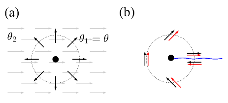
Figure 19: (Color online) $\pi-\pi$ vortex in $\alpha=0$ limit. (a) In $\theta_{1}-\theta_{2}$ representation; black (gray) arrows indicate $\theta_{1}$ ($\theta_{2}$). (b) In $\theta_{+}-\theta_{-}$ representation, the pair of arrows indicate $\theta_{+}$ and $\theta_{-}$, while the wavy line indicates a domain wall. For $\alpha\neq 0$, the FR coupling “squeezes” the $\theta_{+}$ $\pi$-vortex textures into a domain wall of width $\xi\sim 1/Q$. In the presence of an additional molecular $2\pi$ vortex, the domain wall is absent and the composite defect is deconfined.

VIII Local Density Approximation

Because the primary experimental application of our predictions is to degenerate atomic gases it is important to extend our analysis to include the trapping potential $V_{t}({\bf r})$, which in a typical experiment is well-approximated by a harmonic potential. A full analysis of the effect of the trap is beyond the scope of this paper, and here we limit our treatment to a LDA.

Closely related to the WKB approximation landau.QM , LDA amounts to the bulk system predictions, but with the chemical potential replaced by an effective local chemical potential $\mu(r)=\mu-V_{t}(r)$. The validity of the LDA relies on the smoothness of the trap potential, with the criterion that $V_{t}(r)$ varies slowly on the scale of the longest physical length $\lambda$ in the problem, i.e., $(\lambda/V_{t}(r))dV_{t}(r)/dr\ll 1$. Its accuracy can be equivalently controlled by a ratio of the single-particle trap level spacing $\delta E$ to the smallest characteristic energy $E_{c}$ of the studied phenomenon (e.g, the chemical potential, condensation energy, etc.), by requiring $\delta E/E_{c}\ll 1$. For our system the longest natural length scale is the period $2\pi/Q$, Eq. (1) of the finite-momentum atomic condensate inside the AMSF state. Thus, away from the AMSF-ASF phase boundary, where $Q$ vanishes (see Fig. 2), we expect an LDA treatment of the effects of the trap to be trustworthy.

A generalization of a resonant Bose-gas model [Eq. (II)] to include a trap is straightforward, accounted for by the additional Hamiltonian density

$${\cal H}_{\rm trap} = \sum_{\sigma=1,2}V_{t}({\bf r})\hat{\psi}_{\sigma}^{{\dagger}}\hat{\psi}_{\sigma}+2V_{t}({\bf r})\hat{\bm{\phi}}^{{\dagger}}\cdot\hat{\bm{\phi}},$$ (125)

with ${\cal H}\rightarrow{\cal H}+{\cal H}_{\rm trap}$. In the above, for simplicity we specialized to an atomic species-independent trapping potential and approximated the closed-channel molecular trapping potential by twice the atomic one, valid for the interaction range $r_{0}$ (typically less than 50 Å) much smaller than the cloud size $R$ (typically larger than a micron).

Henceforth, to be concrete, we shall focus on an isotropic harmonic trap (although this simplification can easily be relaxed) with

$$V_{t}({\bf r}) = \frac{1}{2}m\omega_{t}^{2}r^{2},$$ (126a)

$$\equiv \mu\frac{r^{2}}{R^{2}},$$ (126b)

the latter expression defining the cloud size $R$. Within LDA, locally the system is taken to be well-approximated as uniform, but with a local chemical potential given by

$$\mu(r) \equiv \mu-\frac{1}{2}m\omega_{t}^{2}r^{2},$$ (127a)

$$= \mu\left(1-\frac{r^{2}}{R^{2}}\right),$$ (127b)

where $\mu$ is the true chemical potential (a Lagrange multiplier) enforcing the total atom number $N$. The spatially varying species $1$ and $2$ chemical potentials are then given by:

$$\mu_{1}(r) = \mu(r)+h,$$ (128a)

$$\mu_{2}(r) = \mu(r)-h,$$ (128b)

with a uniform chemical potential difference $h$ set by the atomic species imbalance SRprl.06 ; SRaop.07 ; FFLOlongLeo .

Consequently, within LDA the system’s energy density is approximated by that of a uniform bulk system [Eq. (20)], with the spatial dependence entering only through $\mu(r)$. The ground-state energy is then simply a volume integral of this energy density. Thus, the phase behavior of a uniform system as a function of the chemical potential, $\mu$, translates into a spatial cloud profile through $\mu(r)$, with the critical phase boundaries $\mu_{c}$ corresponding to critical radii defined by $\mu_{c}=\mu(r_{c},h)$ SRprl.06 ; SRaop.07 . As predicted weddingCakeMI ; SRprl.06 and observed GreinerNature ; Zwierlein06Science ; Partridge06Science ; Shin2006prl ; Navon2009prl in other systems, this leads to a shell-like cloud structure “imaging” of the bulk phase diagram as illustrated in Fig. 20.

Applying this LDA analysis to our system leads to a prediction of rich, magnetic-field, atom-number, and temperature-tunable shell structures in a $p$-wave resonant Bose gas, schematically illustrated in Fig. 21. For a range of atom number, detuning, and temperature admitting the AMSF phase, we expect a cloud shell with an $r$-dependent atomic condensate wavevector $q(r)$, given by

$$q(r) = \alpha m\sqrt{n_{m}(r)},$$ (129a)

$$\approx q_{0}\sqrt{1-\frac{r^{2}}{R^{2}}},\ \ \mbox{for $r_{\rm MSF}<r<r_{\rm ASF}$},\quad$$ (129b)

where $r_{\rm MSF}(T,N,\nu)$ and $r_{\rm ASF}(T,N,\nu)$ are the boundaries of the AMSF shell.

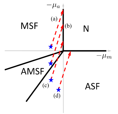
Figure 20: (Color online) $N,\nu,T$-dependent cuts through the bulk phase diagram with increasing radial position $r$ through the atomic cloud. Stars indicate system’s parameters (local chemical potentials $\mu_{a}$, $\mu_{m}$) at the trap center.

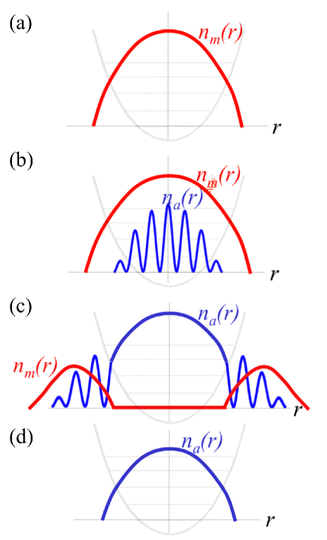
Figure 21: (Color online) Schematic illustration of the shell structure expected in the $p$-wave resonant atomic cloud, corresponding to the phase diagram cuts in Fig. 20.

IX Summary and Conclusions

To summarize, we studied a degenerate gas of two-species bosonic atoms interacting through a $p$-wave FR, as realized, for example, in a ⁸⁵Rb-⁸⁷Rb mixture. We mapped out the corresponding phase diagram and thermodynamic properties of the phases as a function of temperature, atom number, and FR detuning, and analyzed the nature of corresponding phase transitions. We showed that at intermediate detuning such atomic quantum gas generically exhibits an AMSF state with atoms condensed at a finite tunable momentum ${\textbf{\em Q}}(\nu)$ along a direction set by the angular momentum axis of the molecular condensate. This AMSF state undergoes quantum phase transitions described by a quantum de Gennes model into a $p$-wave (orbital spinor-1) MSF and into an $s$-wave ASF at large negative and positive detunings, respectively. A magnetic field can be used to tune the modulation wavevector of the AMSF between zero and a value set by interactions as well as to drive quantum phase transitions in this rich system.

X Acknowledgments

We thank V. Gurarie for discussions, and acknowledge financial support by the National Science Foundation through grants No. DMR-1001240 and MRSEC DMR-0820579. L.R. also acknowledges support by the Miller Foundation and the University of Colorado, and thanks Berkeley Physics Department for its hospitality during the initial part of this work.

Appendix A Order parameter structure

As discussed in the main text, the detailed nature of the AMSF states depends on the structure (the set of reciprocal lattice vectors, ${\textbf{\em Q}}_{n}$) of the finite-momentum atomic order parameter. However, because $\Psi_{{\textbf{\em Q}}_{n}}$ depends on the details of the inter atomic interactions and fluctuations, to determine its form in general is a nontrivial problem, as exemplified by the FFLO problem and the conventional crystallization. However, as seen in Sec.IV, for the case of the AMSF_p state, the problem simplifies considerably as the energy is clearly minimized by a collinear state, with ${\textbf{\em Q}}_{n}$ parallel to $\bm{\Phi}$. Such collinear states fall into two universality classes FFLOlongLeo , represented by the FF-like ff.64 and the LO-like lo.65 single harmonic forms,

$$\Psi_{\sigma}^{\rm FF} =\Psi_{\sigma,{\textbf{\em Q}}_{\sigma}}e^{i{\textbf{\em Q}}_{\sigma}\cdot{\textbf{\em r}}},$$ (130)

$$\Psi_{\sigma}^{\rm LO} =\Psi_{\sigma,{\textbf{\em Q}}}e^{i{\textbf{\em Q}}\cdot{\textbf{\em r}}}+\Psi_{\sigma,-{\textbf{\em Q}}}e^{-i{\textbf{\em Q}}\cdot{\textbf{\em r}}}.$$ (131)

In the FF-like (LO-like) state each species is characterized by a single Q (double $\pm{\textbf{\em Q}}$) momentum, exhibiting a uniform (periodic) atomic density.

Focusing on these two collinear (FF and LO) states, in this appendix we demonstrate that, generically (at least within the mean-field theory), it is the FF state that is energetically selected by the interactions.

To this end, we reexpress the mean-field energy densities for FF and LO in terms of the corresponding eigenmodes, $\Psi_{\pm}^{\pm Q}$, the latter involving two ($\pm Q$) critical modes,

$${\cal E}_{\rm FF} =(\varepsilon_{\textbf{\em Q}}-|\Delta_{\textbf{\em Q}}|)|\Psi_{-}^{Q}|^{2}+\frac{1}{2}\lambda|\Psi_{-}^{Q}|^{4},$$ (132)

$${\cal E}_{\rm LO} =(\varepsilon_{\textbf{\em Q}}-|\Delta_{\textbf{\em Q}}|)(|\Psi_{-}^{Q}|^{2}+|\Psi_{-}^{-Q}|^{2})$$

$$+\frac{1}{2}\lambda(|\Psi_{-}^{Q}|^{2}+|\Psi_{-}^{-Q}|^{2})^{2}+\lambda^{\prime}|\Psi_{-}^{Q}|^{2}|\Psi_{-}^{-Q}|^{2},$$ (133)

where $\lambda=\frac{1}{4}(\lambda_{1}+\lambda_{2}+2\lambda_{12})$ and $\lambda^{\prime}=\frac{1}{4}(\lambda_{1}+\lambda_{2}-2\lambda_{12})$.

These free energies thus show that the energetically preferred form of the AMSF state is determined by the coefficient $\lambda^{\prime}$ of last term in Eq. (133). For $\lambda^{\prime}>0$, that is, $\lambda_{1}+\lambda_{2}>2\lambda_{12}$, the single $Q$ FF-like state is selected. On the other hand, for $\lambda^{\prime}<0$, that is, $\lambda_{1}+\lambda_{2}<2\lambda_{12}$, it is the LO-like state that has the lowest energy.

Combining the above requirement on $\lambda^{\prime}$ for the stability of the LO-like state with the condition for two-species miscibility, $\lambda_{1}\lambda_{2}>\lambda_{12}^{2}$, we find an inequality,

$$\frac{\lambda_{1}+\lambda_{2}}{2}<\lambda_{12}<\sqrt{\lambda_{1}\lambda_{2}}$$ (134)

which for positive couplings $\lambda_{i}$ can be shown to have a zero range of stability. Thus, as advertised, within mean-field approximation it is the single $Q$ FF-like AMSF state that is always energetically selected. Perhaps the LO-like AMSF form can be realized for a metastable atomic gas with $\lambda_{i}<0$, as, for example, realized by a ${}^{87}\text{Rb}$-${}^{85}\text{Rb}$ mixture.

References

• (1) M. H. Anderson, J. R. Ensher, M. R. Matthews, C. E. Wieman, and E. A. Cornell, Science 269, 198 (1995).
• (2) K. B. Davis, M.-O. Mewes, M. R. Andrews, N. J. van Druten, D. S. Durfee, D. M. Kurn, and W. Ketterle, Phys. Rev. Lett. 75, 3969 (1995).
• (3) C. A. Regal, M. Greiner, and D. S. Jin, Phys. Rev. Lett. 92, 040403 (2004).
• (4) M. W. Zwierlein, C. A. Stan, C. H. Schunck, S. M. F. Raupach, A. J. Kerman, and W. Ketterle, Phys. Rev. Lett. 92, 120403 (2004).
• (5) J. Kinast, S. L. Hemmer, M. E. Gehm, A. Turlapov, and J. E. Thomas, Phys. Rev. Lett. 92, 150402 (2004).
• (6) C. Chin, M. Bartenstein, A. Altmeyer, S. Riedl, S. Jochim, J. H. Denschlag, and R. Grimm, Science 305, 1128 (2004).
• (7) G. B. Partridge, K. E. Strecker, R. I. Kamar, M. W. Jack, and R. G. Hulet, Phys. Rev. Lett. 95, 020404 (2005).
• (8) M. W. Zwierlein, J. R. Abo-Shaeer, A. Schirotzek, C. H. Schunck, and W. Ketterle, Nature 435, 1047 (2005).
• (9) E. Timmermans, P. Tommasini, M. Hussein, and A. Kerman, Phys. Rep. 315, 199 (1999).
• (10) K. Dieckmann, C. A. Stan, S. Gupta, Z. Hadzibabic, C. H. Schunck, and W. Ketterle, Phys. Rev. Lett. 89, 203201 (2002).
• (11) K. M. O’Hara, S. L. Hemmer, M. E. Gehm, S. R. Granade, and J. E. Thomas, Science 298, 2179 (2002).
• (12) T. Bourdel, J. Cubizolles, L. Khaykovich, K. M. F. Magalhães, S. J. J. M. F. Kokkelmans, G. V. Shlyapnikov, and C. Salomon, Phys. Rev. Lett. 91, 020402 (2003).
• (13) K. E. Strecker, G. B. Partridge, and R. G. Hulet, Phys. Rev. Lett. 91, 080406 (2003).
• (14) R. A. Duine and H. T. C. Stoof, Physics Reports 396, 115 (2004).
• (15) P. Nozières and S. Schmitt-Rink, J. Low Temp. Phys. 59, 195 (1985).
• (16) C. A. R. Sá de Melo, M. Randeria, and J. R. Engelbrecht, Phys. Rev. Lett. 71, 3202 (1993).
• (17) M. Holland, S. J. J. M. F. Kokkelmans, M. L. Chiofalo, and R. Walser, Phys. Rev. Lett. 87, 120406 (2001).
• (18) Y. Ohashi and A. Griffin, Phys. Rev. Lett. 89, 130402 (2002).
• (19) A. V. Andreev, V. Gurarie, and L. Radzihovsky, Phys. Rev. Lett. 93, 130402 (2004).
• (20) J. Levinsen and V. Gurarie, Phys. Rev. A 73, 053607 (2006).
• (21) V. Gurarie and L. Radzihovsky, Ann. Phys. (NY) 322, 2 (2007).
• (22) T.-L. Ho and R. B. Diener, Phys. Rev. Lett. 94, 090402 (2005).
• (23) V. Gurarie, L. Radzihovsky, and A. V. Andreev, Phys. Rev. Lett. 94, 230403 (2005).
• (24) C.-H. Cheng and S.-K. Yip, Phys. Rev. Lett. 95, 070404 (2005).
• (25) J. P. Gaebler, J. T. Stewart, J. L. Bohn, and D. S. Jin, Phys. Rev. Lett. 98, 200403 (2007).
• (26) J. Zhang, E. G. M. van Kempen, T. Bourdel, L. Khaykovich, J. Cubizolles, F. Chevy, M. Teichmann, L. Tarruell, S. J. J. M. F. Kokkelmans, and C. Salomon, Phys. Rev. A 70, 030702 (2004).
• (27) J. Levinsen, N. R. Cooper, and V. Gurarie, Phys. Rev. A 78, 063616 (2008).
• (28) S. L. Cornish, N. R. Claussen, J. L. Roberts, E. A. Cornell, and C. E. Wieman, Phys. Rev. Lett. 85, 1795 (2000).
• (29) L. Radzihovsky, J. Park, and P. B. Weichman, Phys. Rev. Lett. 92, 160402 (2004).
• (30) L. Radzihovsky, P. B. Weichman, and J. I. Park, Annals of Physics 323, 2376 (2008).
• (31) M. W. J. Romans, R. A. Duine, S. Sachdev, and H. T. C. Stoof, Phys. Rev. Lett. 93, 020405 (2004).
• (32) V. N. Efimov, Sov. J. Nucl. Phys. 12, 589 (1971).
• (33) S. Basu and E. J. Mueller, Phys. Rev. A 78, 053603 (2008).
• (34) J. L. Roberts, N. R. Claussen, S. L. Cornish, E. A. Donley, E. A. Cornell, and C. E. Wieman, Phys. Rev. Lett. 86, 4211 (2001).
• (35) S. Diehl, M. Baranov, A. J. Daley, and P. Zoller, Phys. Rev. B 82, 064509 (2010).
• (36) S. Diehl, M. Baranov, A. J. Daley, and P. Zoller, Phys. Rev. B 82, 064510 (2010).
• (37) N. Syassen, D. M. Bauer, M. Lettner, T. Volz, D. Dietze, J. J. Garcia-Ripoll, J. I. Cirac, G. Rempe, and S. Dürr, Science 320, 1329 (2008).
• (38) H. A. Bethe Handbuch der Physik, second edition, Vol. 24-1, Berlin: Springer (1933), pp. 452-462.
• (39) S. Ejima, M. J. Bhaseen, M. Hohenadler, F. H. L. Essler, H. Fehske, and B. D. Simons, Phys. Rev. Lett. 106, 015303 (2011).
• (40) L. Bonnes and S. Wessel, Phys. Rev. Lett. 106, 185302 (2011).
• (41) M. J. Bhaseen, A. O. Silver, M. Hohenadler, and B. D. Simons, Phys. Rev. Lett. 103, 265302 (2009).
• (42) S. B. Papp, Ph.D. thesis, University of Colorado (2007).
• (43) S. B. Papp, J. M. Pino, and C. E. Wieman, Phys. Rev. Lett. 101, 040402 (2008).
• (44) A. B. Kuklov, Phys. Rev. Lett. 97, 110405 (2006).
• (45) W. V. Liu and C. Wu, Phys. Rev. A 74, 013607 (2006).
• (46) L. Radzihovsky and S. Choi, Phys. Rev. Lett. 103, 095302 (2009).
• (47) J. Stenger, S. Inouye, D. M. Stamper-Kurn, H.-J. Miesner, A. P. Chikkatur, and W. Ketterle, Nature 396, 345 (1998).
• (48) A. Görlitz, T. L. Gustavson, A. E. Leanhardt, R. Löw, A. P. Chikkatur, S. Gupta, S. Inouye, D. E. Pritchard, and W. Ketterle, Phys. Rev. Lett. 90, 090401 (2003).
• (49) M.-S. Chang, C. D. Hamley, M. D. Barrett, J. A. Sauer, K. M. Fortier, W. Zhang, L. You, and M. S. Chapman, Phys. Rev. Lett. 92, 140403 (2004).
• (50) M.-S. Chang, Q. Qin, W. Zhang, L. You, and M. S. Chapman, Nature Physics 1, 111 (2005).
• (51) M. Vengalattore, S. R. Leslie, J. Guzman, and D. M. Stamper-Kurn, Phys. Rev. Lett. 100, 170403 (2008).
• (52) T.-L. Ho, Phys. Rev. Lett. 81, 742 (1998).
• (53) T. Ohmi and K. Machida, J. Phys. Soc. Japan 67, 1822 (1998).
• (54) D. M. Stamper-Kurn, M. R. Andrews, A. P. Chikkatur, S. Inouye, H.-J Miesner, J. Stenger, and W. Ketterle, Phys. Rev. Lett. 80, 2027 (1998).
• (55) M. R. Matthews, D. S. Hall, D. S. Jin, J. R. Ensher, C. E. Wieman, E. A. Cornell, F. Dalfovo, C. Minniti, and S. Stringari, Phys. Rev. Lett. 81, 243 (1998).
• (56) C. K. Law, H. Pu, and N. P. Bigelow, Phys. Rev. Lett. 81, 5257 (1998).
• (57) T.-L. Ho and S. K. Yip, Phys. Rev. Lett. 84, 4031 (2000).
• (58) F. Zhou, Phys. Rev. Lett. 87, 080401 (2001).
• (59) E. Demler and F. Zhou, Phys. Rev. Lett. 88, 163001 (2002).
• (60) R. Barnett, A. Turner, and E. Demler, Phys. Rev. Lett. 97, 180412 (2006).
• (61) S. Mukerjee, C. Xu, and J. E. Moore, Phys. Rev. Lett. 97, 120406 (2006).
• (62) J. Mur-Petit, M. Guilleumas, A. Polls, A. Sanpera, M. Lewenstein, K. Bongs, and K. Sengstock, Phys. Rev. A 73, 013629 (2006).
• (63) A. Lamacraft, Phys. Rev. Lett. 98, 160404 (2007).
• (64) S. Mukerjee, C. Xu, and J. E. Moore, Phys. Rev. B. 76, 104519 (2007).
• (65) S. Folling, A. Widera, T. Muller, F. Gerbier, and I. Bloch, Phys. Rev. Lett. 97, 060403 (2006).
• (66) G. K. Campbell, J. Mun, M. Boyd, P. Medley, A. E. Leanhardt, L. G. Marcassa, D. E. Pritchard, and W. Ketterle, Science 313, 649 (2006).
• (67) R. A. Barankov, C. Lannert, and S. Vishveshwara, Phys. Rev. A 75, 063622 (2007), and references therein.
• (68) A. F. Andreev and I. M. Lifshitz, Zh. Eksp. Teor. Fiz. 56, 2057 (1969) [Sov. Phys. JETP 29, 1107 (1969)].
• (69) G. V. Chester, Phys. Rev. A 2, 256 (1970).
• (70) A. J. Leggett, Phys. Rev. Lett. 25, 1543 (1970).
• (71) E. Kim and M. H. W. Chan, Nature 427, 225 (2004); Science 305, 1941 (2004).
• (72) P. G. de Gennes and J. Prost, The Physics of Liquid Crystals (Oxford University Press, 1995), 2nd ed.
• (73) P. Fulde and R. A. Ferrell, Phys. Rev. 135, A550 (1964).
• (74) A. I. Larkin and Y. N. Ovchinnikov, Sov. Phys. JETP 20, 762 (1965).
• (75) Y. Liao, A. S. C. Rittner, T. Paprotta, W. Li, G. B. Partridge, R. G. Hulet, S. K. Baur, and E. J. Mueller, Nature 467, 567 (2010).
• (76) A. Bianchi, R. Movshovich, C. Capan, P. G. Pagliuso, and J. L. Sarrao, Phys. Rev. Lett. 91, 187004 (2003).
• (77) T. Mizushima, K. Machida, and M. Ichioka, Phys. Rev. Lett. 94, 060404 (2005).
• (78) D. E. Sheehy and L. Radzihovsky, Phys. Rev. Lett. 96, 060401 (2006).
• (79) D. E. Sheehy and L. Radzihovsky, Ann. of Phys. 322, 2 (2007).
• (80) L. Radzihovsky, D. E. Sheehy, Rep. Prog. Phys. 73, 076501 (2010).
• (81) H. J. Kimble, Quantum fluctuations in quantum optics - squeezing and related phenomena, les Houches, Session LIII, 1990 (Elsvier, 1992) and references therein.
• (82) C. Orzel, A. K. Tuchman, M. L. Fenselau, M. Yasuda, and M. A. Kasevich, Science 291, 2386 (2001).
• (83) L. Radzihovsky and A. Vishwanath, Phys, Rev. Lett. 103, 010404 (2009).
• (84) L. Radzihovsky, Phys. Rev. A 84, 023611 (2011).
• (85) For unequal masses FR interaction is given by $H_{FR}=\alpha\hat{\bm{\phi}}^{{\dagger}}\cdot\left[\frac{m_{1}}{m_{1}+m_{2}}\hat{\psi}_{1}(-i{\bm{\nabla}})\hat{\psi}_{2}-\frac{m_{2}}{m_{1}+m_{2}}\hat{\psi}_{2}(-i{\bm{\nabla}})\hat{\psi}_{1}\right]+h.c.$ as required to preserve Galilean invariance.
• (86) C. A. Regal, C. Ticknor, J. L. Bohn, and D. S. Jin, Phys. Rev. Lett. 90, 053201 (2003).
• (87) L. D. Landau and E. M. Lifshitz, Quantum Physics (Butterworth-Heinemann, Oxford, 1980).
• (88) B. D. Esry, C. H. Greene, J. P. Burke, Jr., and J. L. Bohn, Phys. Rev. Lett. 78, 3594 (1997).
• (89) Y. W. Lee and Y. L. Lee, Phys. Rev. B. 70, 224506 (2004).
• (90) M. P. A. Fisher, P. B. Weichman, G. Grinstein, and D. S. Fisher, Phys. Rev. B. 40, 546 (1989).
• (91) J. W. Negele and H. Orland, Quantum Many-Particle Systems (Addison-Wesley, 1988).
• (92) S. Sachdev and N. Read, Int. J. Mod. Phys. B 5, 219 (1991); S. Sachdev, Lecture Notes at the Les Houches Summer School on “Modern theories of correlated electron systems” (2009), Lecture Notes at the Mahabaleshwar Condensed Matter School, International Center for Theoretical Sciences, India (2009), arXiv:1002.3823.
• (93) Chao-Ming Jian and Hui Zhai, Phys. Rev. B 84, 060508 (2011).
• (94) For simplicity it is convenient to first consider a homogeneous bulk system or a “box” trap, and take into account the trap-induced local inhomogeneity using LDA, valid for large condensates and smooth trapping potential.
• (95) In the absence of an optical potential or quenched disorder that can “localize” atom number and induce Mott- or Bose-glass insulating phases, only Bose-condensed, superfluid ground states are expected at zero temperature.
• (96) $U_{N}(1)$ and $U_{\Delta N}(1)$ symmetries are associated with the total atom number $N=N_{1}+N_{2}+2N_{m}$ and difference $\Delta N=N_{1}-N_{2}$ conservations, respectively.
• (97) More accurately, it is not $g_{2}$ but T-matrix, i.e., scattering length $a$’s that matter.
• (98) In the context of conventional spinor condensate, the polar state is also termed “nematic” or “antiferromagnetic” superfluid.
• (99) P. M. Chaikin and T. C. Lubensky, Principles of Condensed Matter Physics (Cambridge University Press, 1995).
• (100) To keep the form of the Landau free energy simple, one needs to be sufficiently close to the transition boundaries (but staying outside the critical region, where local Landau mean-field expansion fails) to allow a local expansion in the order parameters.
• (101) K.-S. Liu and M. E. Fisher, J. Low Temp. Phys. 10, 655 (1973).
• (102) J.M. Kosterlitz, D.R. Nelson, and M. E. Fisher, Phys. Rev. B 13, 412 (1976).
• (103) P. Calabrese, A. Pelissetto, and E. Vicari, Phys. Rev. B 67, 054505 (2003).
• (104) I. Bloch, J. Dalibard, W. Zwerger, Rev. Mod. Phys. 80, 885 (2008).
• (105) B. I. Halperin, T. C. Lubensky, and S. K. Ma, Phys. Rev. Lett. 32, 292 (1974).
• (106) S. Coleman and E. Weinberg, Phys. Rev. D 7, 1888 (1973).
• (107) D. Podolsky, S. Chandrasekharan, and A. Vishwanath, Phys. Rev. B 80, 214513 (2009).
• (108) E. Babaev, Phys. Rev. Lett. 89, 067001 (2002).
• (109) N. D. Mermin, Rev. Mod. Phys. 51, 591 (1979).
• (110) B. DeMarco, C. Lannert, S. Vishveshwara, and T.-C. Wei, Phys. Rev. A 71, 063601 (2005).
• (111) M. Greiner, O. Mandel, T. Esslinger, T. W. Hänsch, and I. Bloch, Nature 415, 39 (2002).
• (112) M. W. Zwierlein, A. Schirotzek, C. H. Schunck, and W. Ketterle, Science 311, 492 (2006).
• (113) G. B. Partridge, W. Li, R. I. Kamar, Y. Liao, and R. G. Hulet, Science 311, 503 (2006).
• (114) Y. Shin, M. W. Zwierlein, C. H. Schunck, A. Schirotzek, and W. Ketterle, Phys. Rev. Lett. 97, 030401 (2006).
• (115) S. Nascimbène, N. Navon, K. J. Jiang, L. Tarruell, M. Teichmann, J. McKeever, F. Chevy, and C. Salomom, Phys. Rev. Lett. 103, 170402 (2009).