A Replica Inference Approach to Unsupervised Multi-Scale Image Segmentation

Abstract

We apply a replica inference based Potts model method to unsupervised image segmentation on multiple scales. This approach was inspired by the statistical mechanics problem of “community detection” and its phase diagram. Specifically, the problem is cast as identifying tightly bound clusters (“communities” or “solutes”) against a background or “solvent”. Within our multiresolution approach, we compute information theory based correlations among multiple solutions (“replicas”) of the same graph over a range of resolutions. Significant multiresolution structures are identified by replica correlations as manifest in information theory overlaps. With the aid of these correlations as well as thermodynamic measures, the phase diagram of the corresponding Potts model is analyzed both at zero and finite temperatures. Optimal parameters corresponding to a sensible unsupervised segmentation correspond to the “easy phase” of the Potts model. Our algorithm is fast and shown to be at least as accurate as the best algorithms to date and to be especially suited to the detection of camouflaged images.

I Introduction

“Image segmentation” refers to the process of partitioning a digital image into multiple segments based on certain visual characteristics book1 ; book2 ; book3 . Image segmentation is typically used to locate objects and boundaries in images. The result of image segmentation is a set of segments that collectively cover the entire image or a set of extracted contours of the image. This problem is challenging (see, e.g., Fig. (1)) and important in many fields. Examples of its omnipresent use include, amongst many others, medical imaging medical (e.g., locating tumors and anatomical structure), face recognition face , fingerprint recognition fingerprint , and machine vision mechine . Numerous algorithms and methods have been developed for image segmentation. These include thresholding thresholding , clustering clustering , compression compression and histogram based histogram approaches, edge detection edge , region growing region , split and merge split , gradient flows and partial differential equation based approaches kim ; levelset , graph partitioning methods and normalized cuts graphpartition ; normalizedcuts , Markov random fields and mean field theories markov1 ; markov2 ; markov3 ; markov4 , watershed transformation watershed , random walks randomwalks , isoperimetric methods isoperimetric , neural networks neural , and a variety of other approaches, e.g., model ; multi ; semi .

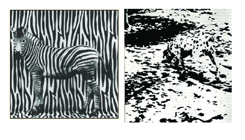
Figure 1: Examples of currently challenging problems in image segmentation. Left: The left image is that of zebra (courtesy of Ref.berkeley-zebra ) with the a similar“stripe” background. Right: The image on the right is that of a dalmatian dog dalmatian . Most people do not initially recognize the dog before given clues as to its presence. Once the dog is seen it is nearly impossible to perceive the image in a meaningless way. dalmatian

In this work, we will apply a “community detection” algorithm to image segmentation. This method belongs to the graph partitioning category. Community detection newman ; fortunato ; newman2 ; gmnn seeks to identify groups of nodes densely connected within their own group (“community”) and more weakly connected to other groups. A solution enables the partition of a large physically interacting system into optimally decoupled communities. The image is then divided into different regions (“communities”) based on a certain criterion, and each resulting region corresponds to an object in the original image.

It is notable that by virtue of its graph theoretical nature, community detection is suited for the study of arbitrary dimensional data. However, unlike general high dimensional graphs, images are two (or three) dimensional. Thus, real images are far simpler than higher dimensional data sets as, e.g., evinced by the four color theorem stating that four colors suffice to mark different neighboring regions in a segmentation of any two dimensional image. Thus, geometrical (and topological) constraints can be used to further improve the efficiency of the bare graph theoretical method. In glass1 ; glass2 , in the context of analyzing structures of complex physical systems such as glasses, we used geometry dependent physical potentials to set the graph weights in various two and three dimensional systems. In the case of image segmentation, in the absence of underlying physics, we will invoke geometrical cut-off scales.

In this work, we will discuss “unsupervised” image segmentation. By this term, we allude to a general multi-purpose segmentation method based on a general physical intuition. The current method does not take into account initial “training” of the algorithm- i.e., provide the system with known examples in which specific patterns are told to correspond to specific objects. We leave the study of supervised image segmentation and more sophisticated extensions of our inference procedure to a future work. One possible avenue which can be explored is the use of inference beyond that relating to different “replicas” in the simple form discussed in this manuscript that is built on prior knowledge (and prior probabilities in a Bayesian type analysis) of expected patterns in the studied images.

We will, specifically, apply the multiresolution community detection method, first introduced in peter1 , to investigate the overall structure at different resolutions in the test images. Similar to peter1 , we will employ information based measures (e.g., the normalized mutual information and the variation of information) to determine the significant structures at which the “replicas” (independent solutions of the same community detection algorithm) are strongly correlated. With the aid of these information theory correlations, we illustrate how we may discern structures at different pertinent resolutions (or spatial scales). An image may be segmented at different levels of detail and scales by setting the resolution parameters to these pertinent values. We demonstrate in a detailed study of various test cases, how our method works in practice and the resulting high accuracy of our image segmentation method.

II Outline

The outline of our work is as follows. In Section III, we introduce the Potts model representation of image segmentation and Potts model Hamiltonians that we will use. These Hamiltonians were earlier derived for graph theory applications. In Section IV, we discuss how we represent images as graphs. In Section V, we briefly define the key concepts of trials and replicas which are of great importance in our approach. In Sec. VI, we present our community detection algorithm. In Sec. VII, we discuss the multiresolution method and the information based measures. In Section VIII, we illustrate how replica correlations may be used to set graph weights. For the benefit of the reader, we compile the list of parameters in Section IX. We discuss the computational complexity of our method in Section X. In Sec. XI, we provide in silico “experimental results” of our image segmentation method when applied to many different examples. These examples include, amongst others, the Berkeley image segmentation and the Microsoft Research Benchmarks. We conclude in Sec. XII with a summary of our results. Specific aspects are further detailed in the appendices.

III Potts Models

In what follows, we will briefly elaborate on our particular Potts model representations of images and the corresponding Hamiltonians (energy or cost functions).

III.1 Representation

As is well appreciated, different objects in an image or more general communities in complex graph theoretical problems are ultimately denoted by a “Potts type” potts variable $\sigma_{i}$. That is, if node $i$ lies in a community number $w$ then $\sigma_{i}=w$. If there are $q$ communities in the graph then $\sigma_{i}$ can assume values $1\leq\sigma_{i}\leq q$. A state $\{\sigma_{s}\}_{s=1}^{N}$ corresponds to a particular partition (or segmentation) of the system into $q$ communities (or objects). In the context of image segmentation, Potts model representations can, e.g., also be found in pottsmodel1 ; pottsmodel2 ; pottsmodel3 ; pottsmodel4 .

III.2 Potts model Hamiltonian for unweighted graphs

In peter2 , a particular Potts model Hamiltonian was introduced for community detection. The ground states of this Hamiltonian (or lowest energy states) correspond to optimal partition of the nodes into communities. This Hamiltonian does not involve a comparison relative to random graphs (“null models”) fortunato and as such was free of the “resolution limit” problems fortunato ; rlimit1 ; rlimit2 wherein the number of found communities or objects scaled with the system size in a way that was independent of the actual system studied. In what follows below, there are $N$ elementary nodes in a graph (or pixels in an image), we consider general unweighted graphs in which any pair of nodes may be either linked with a uniform weight or not linked at all. Specifically, a link between sites $i$ and $j$ is associated with edge weights $A_{ij}$ and $J_{ij}$. In these unweighted graphs, $A_{ij}$ is an element of the adjacency matrix. That is, $A_{ij}=1$ if nodes $i$ and $j$ are connected by an edge and $A_{ij}=0$ otherwise. The weights $J_{ij}=(1-A_{ij})$.

The goal of the general (or “absolute”) Potts model Hamiltonian peter2 was to energetically favor any pair of linked nodes to be in the same community, to penalize for a pair of unlinked nodes to be in the same community and conversely for nodes in different communities (penalize for having two linked nodes be in different communities and favor disjoint nodes being in different communities). Putting all of these bare energetic considerations together (sans any comparisons to random graphs), the resulting Potts model Hamiltonian (or energy function) for a system of $N$ nodes simplifies to peter2 ; explain_solute

$${\cal{H}}(\{\sigma_{s}\}_{s=1}^{N})=-\frac{1}{2}\sum_{i\neq j}(A_{ij}-\gamma J_{ij})\delta(\sigma_{i},\sigma_{j}).$$ (1)

In Eq.(1), we emphasize the dependence of the Hamiltonian on the $N$ different variables $\{\sigma_{s}\}$ at each lattice site $s$ (each of which can assume $q$ values). In what follows, the dependence of the Hamiltonian on $\{\sigma_{s}\}_{s=1}^{N}$ will always be understood.

The Kronecker delta $\delta(\sigma_{i},\sigma_{j})=1$ if $\sigma_{i}=\sigma_{j}$ and $\delta(\sigma_{i},\sigma_{j})=0$ if $\sigma_{i}\neq\sigma_{j}$. In this Hamiltonian, by virtue of the $\delta_{\sigma_{i}\sigma_{j}}$ term, each spin $\sigma_{i}$ interacts only with other spins in its own community. As such, the resulting model is local– a feature that enables high accuracy along with rapid convergence peter2 .

As noted above, minimizing this Hamiltonian corresponds to identifying strongly connected clusters of nodes. The parameter $\gamma$ is the so called “resolution parameter” which adjusts the relative weights of the linked and unlinked edges, as in Eq. (1). This is easily seen by inspecting Eq.(1). A high value of $\gamma$ leads to forbidding energy penalties unless all intra-community nodes “attract” one another and lie in the same community. By contrast, $\gamma=0$ does not penalize the inclusion of any additional nodes in a given community and the lowest energy solution generally corresponds to the entire system.

III.3 Potts Model Hamiltonian for Weighted Graphs

In weighted graphs, we assign edges between nodes with the respective weights based on the interaction strength (e.g., the (dis-) similarity of the intensity or color defines the edge weight in image segmentation problem). Specifically, in image segmentation problems, we determine (based on, e.g., color or intensity differences) the weight $V_{ij}$ between each member of a node pair. We then shift each such value by an amount set by a background $\bar{V}$, i.e., $V_{ij}^{\prime}=(V_{ij}-\bar{V})$. The subtraction relative to the background of $\bar{V}$ allows for our community detection algorithm to better partition the network of pixels. In principle, this background can be set to be spatially non-uniform. However, in this work we set $\bar{V}$ to be a constant. Thus, we generalize the earlier model of peter1 in Eq. (1) by the inclusion of a background $\bar{V}$ and by allowing for continuous weights $V_{ij}$ instead of discrete weights that are prevalent in graph theory. The resulting Hamiltonian glass1 ; glass2 reads

$${\cal{H}}=\frac{1}{2}\sum_{a=1}^{q}(V_{ij}-\bar{V})\Big{[}\Theta(\bar{V}-V_{ij})+\gamma\Theta(V_{ij}-\bar{V})\Big{]}\delta(\sigma_{i},\sigma_{j}).$$ (2)

The form of this Hamiltonian and that of Eq. (1) was inspired by positive and negative energy terms that favor the formation of tightly bound clusters (or “solutes”) that are more weakly coupled to their surroundings explain_solute . Similar to the important effects of the solute found in physical systems mossa , the Hamiltonian of Eq.(2) captures all interactions in the system explain_solute . Earlier glass1 ; glass2 ), we invoked the Hamiltonian of Eq. (2) to analyze static and dynamic structures in glasses.

In Eq. (2), the number of communities $q$ may be specified from the input or left arbitrary and have the algorithm decide by steadily increasing the number of communities $q$ for which we have low energy solutions. The Heavyside functions $\Theta(x)$ “turns on” or “off” the edge designation [$\Theta(x>0)=1$ and $\Theta(x<0)=0$] relative to the aforementioned background $\bar{V}$. As before, minimizing the Hamiltonian of Eq. (2) corresponds to identifying strongly connected clusters of nodes.

While in Eq. (1 (or Eq. 2),) the input concerns two-point ($p=2$) edge weights $V_{ij}$ (or $A_{ij}$) , it is, of course, possible to extend these Hamiltonian to allow for more general motifs (such as $p=3$ node triangles) and include $p\geq 3$ point weights $V_{ijk}$ (and extensions thereof). These correspond to $p$ spin interactions. In the current study, however, we limit ourselves to $p=2$ node weights.

IV Casting Images as Networks

We will now detail how we translate images into networks with general edge weights that appear in Eqs.(1, 2). We will represent pixels as the nodes in a graph. Edge weights define the (dis-) similarity between the neighborhood pixels.

Images may be broadly divided into two types: (a) those with the uniform and (b) those with varying intensity. “Uniform intensity” means that the entire object or each component is colored by one intensity or color. By the designation of “varying intensity”, we allude to objects or components that exhibit alternating intensities or colors, e.g., the stripes and spots seen in Fig. (1).

Regarding the above two types of images, two different methods may be employed to define the edge weights: (i) The intensity/color difference between nodes is defined as the edge weight in images with uniform intensity. (ii) The overlap between discrete Fourier transforms of blocks is defined as the edge weight in images with varying intensity. The second method is designed to distinguish the target and the background by their specific frequencies. We will detail both methods below in Sec. IV.1 (where we discuss images with uniform intensities) and Sec. IV.2 (spatially varying intensities).

IV.1 Edge definition for images with uniform intensity

For images of uniform intensity, we will define edges based on the color (dis-) similarity. For the unweighted Potts model of Eq. (1), we will assign an edge between two pixels ($i$ and $j$ ) if the “color” difference ($D_{ij}$) between them is less than some threshold ($\bar{V}$). That is,

$$A_{ij}=\Theta(\bar{V}-D_{ij}).$$ (3)

For weighted Potts model in Eq. (2), we will, as we will elaborate on momentarily, set the weights $V_{ij}$ to be the “color” difference ($D_{ij}$) between nodes $i$ and $j$, i.e.,

$$V_{ij}=D_{ij}.$$ (4)

As seen from the energy functions of Eqs. (1, 2), a large dis-similarity $V_{ij}$ favors nodes $i$ and $j$ being in different clusters.

A grey scale image is an image that in which the value of each pixel carries only intensity information. Images of this sort are composed exclusively of shades of gray, varying from black at the weakest intensity ($I=0$) to white at the strongest ($I=255$). For a grey-scale image, the “color” difference is the absolute value of the intensity difference, i.e.,

$$D_{ij}=|I_{i}-I_{j}|.$$ (5)

A “color image” is an image that includes color information for each pixel. Each pixel contains three color components: red, green and blue (or RGB). The value of the intensity of each of these three components may attain any of $2^{8}$ values (any integer in the interval $[0,255]$). For a color-scale image, we define the “color” difference as the average of the differences between the color components red, green and blue. That is, with $R_{i},G_{i},$ and $B_{i}$ respectively denoting the strengths of the red, green, and blue color components at site $i$, we set

$$D_{ij}=\frac{1}{3}(|R_{i}-R_{j}|+|G_{i}-G_{j}|+|B_{i}-B_{j}|).$$ (6)

We do not store edges between every pair of nodes. Rather, edges connect nodes whose distance is less than a tunable value $\Lambda$.

IV.2 Edge definition for images with varying intensities

Typically, images with varying intensities contain different patterns. To separate these patterns, we construct a “block-structure” containing the quintessential pattern information. We next introduce a method to divide blocks and then elaborate on two different ways to connect edges between blocks.

General contending pertinent scales may be determined by, e.g., examining the peaks of the Fourier transform of an entire image (whose location yields the inverse wave-length and whose width reveals the corresponding spatial extent of these modulations). While such simple transforms may aid optimization in determining candidate parameter scales, our algorithm goes far beyond such simple global measures.

IV.2.1 Overlapping blocks

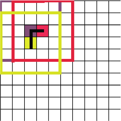
Figure 2: [Color Online.] An example of overlapping blocks. The block size is $L_{x}\times L_{y}=5\times 5$. The nearest neighbor of the block enclosed by “purple” in x-direction is the one enclosed by “red”, and its nearest neighbor in y-direction is the one enclosed by “yellow”. They are connected due to the nearest neighbor condition.

We will divide an entire image of size $N=N_{x}\times N_{y}$ into $N$ overlapping blocks. These blocks are centered about each (of the $N$) pixels and are of size $L_{x}\times L_{y}$. The dimensions of the individual blocks are, generally, far smaller than that of the entire system, $L_{x,y}\ll N_{x,y}$. General scales can be gleaned from a Fourier transform of the entire image.

To construct the connection matrix between the blocks, we connect edges between each pair of blocks and set the distance between the nearest block pair to be $1$. This choice has the benefit of overlapping the nearest neighbor blocks, which share more commons. Fig. 2 gives a schematic plot of the “overlapping block” structure.

IV.2.2 Average intensity difference between blocks

Following the construction of the overlap blocks structure, we next compute the average intensity of each block and connect the edges between blocks based on the difference. In this case, each block can be treated as a “super-node” which contains the pattern information of the studied image.

To further incorporate geometrical scales, we multiply the edge weights by $\exp(-|{\bf{r}}_{m}-{\bf{r}}_{n}|/\ell)$ (where $\ell$ is a tunable length scale and the vectors ${\bf{r}}_{m}$ and ${\bf{r}}_{n}$ denote the spatial locations of points $m$ and $n$). We remind the reader that there are $N$ basic blocks and thus $N$ possible values of $m$ (and $N$ possible values of $n$). We will set in Eq. (2), the weights $V_{mn}$ between block $m$ and $n$ to be

$$V_{mn}=\frac{D_{mn}\exp(-|{\bf{r}}_{m}-{\bf{r}}_{n}|/\ell)}{L_{x}L_{y}},$$ (7)

where

$$D_{mn}=(1-\delta(m,n))|\sum_{i=0}^{i=L_{x}-1}\sum_{j=0}^{j=L_{y}-1}(I^{m}(i,j)-I^{n}(i,j))|.$$ (8)

As seen in Eq. (8), $D_{mn}$ is the sum of the absolute values of the intensity differences between blocks $m$ and $n$ with each of these blocks being of size $L_{x}\times L_{y}$. In Eq. (7), $|{\bf{r}}_{m}-{\bf{r}}_{n}|$ is the physical distance between block $m$ and $n$ (i.e., the distance between the central nodes of each block).

The geometrical factor of ($\exp(-|{\bf{r}}_{m}-{\bf{r}}_{n}|/\ell)$) in Eq. (7) with a tunable length scale $\ell$ can be set to prefer (and, as we will illustrate also to detect) certain scales in the image. This enables the algorithm to detect clusters of varying sizes that contain rich textures.

IV.2.3 Fourier amplitude derived weights

As it is applied to image segmentation, the utility of Fourier transformations is well appreciated. We next discuss how to invoke these in our Potts model Hamiltonian. To highlight their well known and obvious use, we note that, e.g., the stripes of the zebra in Fig. 1 contain wave-vectors which are different from those of the more uniformly modulated background. Thus, a spatially local Fourier transform of this image may distinguish the zebra from the background. We will now invoke Fourier transforms in a general way in order to determine the edge weights in our network representation of the image.

With the preliminaries of setting up the block structure in tow, we now apply a discrete Fourier transform inside each block. Rather explicitly, excluding the spatial origin, the local discrete $2-D$ Fourier transform of a general quantity $f_{m}$ within block $m$ with internal Cartesian coordinates $(a,b)$ is

$$F_{m}(k,l)=\sum_{a=0}^{L_{x}-1}\sum_{b=0}^{L_{y}-1}f_{m}(a,b)e^{-2\pi i(\frac{ka}{L_{x}}+\frac{lb}{L_{y}})}-f_{m}(0,0).$$ (9)

The wave-vector components $k=0,1,...,L_{y}-1$ and $l=0,1,...,L_{x}-1$. In applications, we set, for grey-scale images, $f_{m}(a,b)$ to be the intensity $I$ at site $(a,b)$ in block $m$ (a whose location relative to the origin of the entire image we denote by ${\bf r}_{ab;m}$). That is, $f_{m}(a,b)=I({\bf r}_{ab;m})$. In color images, we set $f$ to be the average over the intensity of the red, green and blue components: $f(a,b)=\frac{1}{3}(R(a,b)+G(a,b)+B(a,b))$. We fix the couplings $J_{mn}$ between blocks $m$ and $n$ to be

$$J_{mn}=\sum_{k=0}^{L_{x}-1}\sum_{l=0}^{L_{y}-1}|F_{m}^{*}(k,l)F_{n}(k,l)|.$$ (10)

We connect blocks whose spatial separation is less than the aforementioned tunable cutoff distance $\Lambda$ by links having edge weights $V_{mn}$. In practice, we fixed $\Lambda$. With Eq. (10) in hand, we set

$$V_{mn}=(\delta(m,n)-1)J_{mn}\exp(-|{\bf{r}}_{m}-{\bf{r}}_{n}|/\ell)$$ (11)

in Eq. (2). In this case, the background $\bar{V}$ would be negative.

When inverting the sign of the left hand side of Eq.(11) (shown in Appendix C), our algorithm will be also suited for the detection of changing objects against a more uniform background.

We now briefly comment on the relation between the Fourier space overlaps and weights in Eqs.(10,11) and the real space overlaps and weights in Eqs.(7,8). It is notable that in Eq.(10), we sum over the modulus of the products of the Fourier amplitudes. By Parseval’s theorem, sans the modulus in the summation in Eq.(10), $J_{mn}$ would be identical to the overlap in real space between $f_{m}$ and $f_{n}$. Such real space overlaps directly relate to the real-space overlaps in Eq.(8) [following a replacement of the absolute value in Eq.(8) by its square and an overall innocuous multiplicative scale factor]. Thus, without the modulus in Eq.(10), the Fourier space calculation outlined above affords no benefit over its real space counter-part. Physically, the removal of the phase factors when performing the summation in Eq.(10) avoids knowledge of the relative location of the origins between different blocks. This allows different regions of a periodic pattern to be strongly correlated and clumped together. By contrast, for a periodic wave of a particular wave-vector, the real space overlaps between blocks $m$ and $n$ may vanish when the origins of blocks $m$ and $n$ are displaced by a real space distance that is equal to half of the wave-length of the periodic wave along the modulation direction. Thus, the real space weights as derived from Eqs.(7,8) may vanish when the corresponding Fourier space derived weights (Eqs.(10,11)) are sizable.

It is possible to improve on the simple Fourier space derived weights by a general wavelet analysis.

V Definitions: Trials and Replicas

In the following sections, we will discuss our specific algorithms for (i) community detection and (ii) multi-scale community detection. Before giving the specifics of our algorithms, we wish to introduce two concepts on which our algorithms are based. Both pertain to the use of multiple identical copies of the same system (image) which differ from one another by a permutation of the site indices. Thus, whenever the time evolution may depend on sequentially ordered searches for energy lowering moves (as it will in our greedy algorithm), these copies may generally reach different final candidate solutions. By the use of an ensemble of such identical copies, we can attain accurate result as well as determine information theory correlations between candidate solutions and infer from these a detailed picture of the system.

In the definitions of “trials” and “replicas” given below, we build on the existence of a given algorithm (any algorithm) that may minimize a given energy or cost function. In our particular case, we minimize the Hamiltonian of Eqs. (1, 2).

$\bullet$ Trials. We use trials alone in our bare community detection algorithm peter1 ; peter2 . We run the algorithm on the same problem $t$ independent times. This may generally lead to different contending states that minimize Eqs. (1, 2). Out of these $t$ trials, we will pick the lowest energy state and use that state as the solution.

$\bullet$ Replicas. We use both trials and replicas in our multi-scale community detection algorithm peter2 . Each sequence of the above described $t$ trials is termed a replica. When using “replicas” in the current context, we run the aforementioned $t$ trials (and pick the lowest solution) $r$ independent times. By examining information theory correlations between the $r$ replicas we infer which features of the contending solutions are well agreed on (and thus are likely to be correct) and on which features there is a large variance between the disparate contending solutions that may generally mark important physical boundaries. We will compute the information theory correlations within the ensemble of $r$ replicas. Specifically, information theory extrema as a function of the scale parameters, generally correspond to more pertinent solutions that are locally stable to a continuous change of scale. It is in this way that we will detect the important physical scales in the system.

These definitions might seem fairly abstract for the moment. We will flesh these out and re-iterate their definition anew when detailing our specific algorithms to which we turn next.

VI The community detection algorithm

Our community detection algorithm for minimizing Eqs. (1, 2) follows four steps peter2 .

(1) We partition the nodes based on a “symmetric” or “fixed q” initialization ($q$ is the number of community).

$\bullet$ “Symmetric” initialization alludes to an initialization wherein each node forms its own community (and thus, initially, there are $q=N$ communities).

$\bullet$ “Fixed q” initialization corresponds to a random initial distribution of all nodes into q communities.

For the application of image segmentation, “symmetric” initialization is used for the “unsupervised” case. In this case, the algorithm does not know what to look for, thus the “symmetric” initialization provides the advantage of no bias towards a particular community. The algorithm will decide the number of community $q$ by merging nodes for which we have lower energy solution.

“Fixed q” initialization may be used in a “supervised” image segmentation. The community membership of individual node will be changed to lower the solution energy. One has to decide how much information is needed by observing the original image and enter the number of communities $q$ as an input. Different levels of information correspond to different number of communities $q$. For instance, if only one target needs to be identified, $q=2$ is enough. The $q$ communities include the target and background.

In the following sections, we will use the “unsupervised” image segmentation and let the algorithm decide the community number $q$.

(2) Next, we sequentially “pick up” each node and place it in the community that best lowers the energy of Eqs. (1, 2) based on the current state of the system.

(3) We repeat this process for all nodes and continue iterating until no energy lowering moves are found after one full cycle through all nodes.

(4) We repeat these processes “t” times (trials) and select the lowest energy result as the best solution.

VII Multi-scale networks

After determining for the adjacency matrix in Sec. IV.1 and Sec. IV.2, we now turn to the-so called “resolution parameter” ($\gamma$) in Eq. (1)/Eq. (2). In peter1 , we introduced the multiresolution algorithm to select the best resolution. Our multi-scale community detection was inspired by the use of overlap between replicas in spin-glass physics. In the current context, we employ information-theory measures, to examine contending partitions for each system scale. Decreasing $\gamma$, the minima of Eqs. (1, 2) lead to solutions progressively lower intra-community edge densities, effectively “zooming out” toward larger structures. We determine all natural graph scales by identifying the values of $\gamma$ for which the earlier mentioned “replicas” exhibit extrema in the average of information theory overlaps such as the normalized mutual information ($I_{N}$) and the variation of information ($V$) when expressed as functions of $\gamma$, $\ell$. The extrema and plateau of the average information theory overlaps as a function of $\gamma$, $\ell$ over all replica pairs indicate the natural network scales peter1 . The replicas can be chosen to be identical copies of the same system for the detection of static structures, e.g., the image segmentation.

We will briefly introduce the information theory measures in the following section.

VII.1 Information theory measures

The normalized mutual information $I_{N}$ and the variation of information $V$ are the accuracy parameters which are employed to calculate the similarity (or overlap) between replicas.

We begin with a list of definitions of the information theory overlaps as they pertain to community detection.

$\bullet$ Shannon Entropy: If there are $q$ communities in a partition $A$, then the Shannon entropy is

$$H_{A}=-\sum_{a=1}^{q}\frac{n_{a}}{N}\log_{2}\frac{n_{a}}{N},$$ (12)

where $\frac{n_{a}}{N}$ is the probability for a randomly selected node to be in a community $a$, $n_{a}$ is the number of nodes in community $a$ and $N$ is the total number of nodes.

$\bullet$ Mutual Information:

The mutual information $I(A,B)$ between partitions found by two replicas $A$ and $B$ is

$$I(A,B)=\sum_{a=1}^{q_{A}}\sum_{b=1}^{q_{B}}\frac{n_{ab}}{N}\log_{2}\frac{n_{ab}N}{n_{a}n_{b}},$$ (13)

where $n_{ab}$ is the number of nodes of community $a$ of partition $A$ that are shared with community $b$ of partition $B$, $q_{A}$ (or $q_{B}$) is the number of communities in partition $A$ (or $B$) and $n_{a}$ (or $n_{b}$) is defined the same as before, i.e., the number of nodes in community $a$ (or community $b$).

$\bullet$ Variation of information:

The variation of information $(0\leq V(A,B)\leq\log_{2}N)$ between two partitions $A$ and $B$ is given by

$$V(A,B)=H_{A}+H_{B}-2I(A,B).$$ (14)

$\bullet$ Normalized Mutual Information:

The normalized mutual information $0\leq I_{N}(A,B)\leq 1$ is

$$I_{N}(A,B)=\frac{2I(A,B)}{H_{A}+H_{B}}.$$ (15)

Now, here is a key idea employed in peter1 which will be of great use in our image segmentation analysis: when taken over an entire ensemble of replicas, the average $I_{N}$ or $V$ indicates how strongly a given structure dominates the energy landscape. High values of $I_{N}$ (or low values of $V$) corresponds to more dominate and thus more significant structure. From a local point of view, at resolutions where the system has well-defined structure, a set of independent replicas should be highly correlated because the individual nodes have strongly preferred community memberships. Conversely, for resolutions “in-between” two strongly defined configurations, one might expect that independent replicas will be less correlated due to “mixing” between competing divisions of the graph.

VII.2 The application of the multiresolution algorithm for a hierarchal network example

We will shortly illustrate how the multiresolution algorithm peter1 works in practice by presenting an example of the multiresolution algorithm as it is applied to a hierarchal test system of $N=1024$ nodes.

To begin the multiresolution algorithm, we need to specify the number of replicas $r$ at each test resolution, the number of trials per replica $t$, and the starting and ending resolution $[\gamma_{0},\gamma_{f}]$. Usually, the number of replicas is $8\leq r\leq 12$, the number of trials is $2\leq t\leq 20$. As detailed in Section V, we select the lowest energy solution among the $t$ trials for each replica. The initial states within each of the replicas and trials are generated by reordering the node labels in the “symmetric” initialized state of one node per community. These permutations $P$ simply reorder the node numbers $(1,2,3,...,i,...,N)\to(P1,P2,...,PN)$ (with $Pi$ the image of $i$ under a permutation) and thus lead to a different initial state.

(1) The algorithm starts from the initialization of the system described in item (1) of Section VI.

(2) We then minimize Eq. (1) independently for all replicas at a resolution $\gamma=\gamma_{i}\in[\gamma_{0},\gamma_{f}]$ as described in Section VI. Initially $i=0$ (i.e., $\gamma=\gamma_{0}$).

(3) The algorithm then calculates the average inter-replica information measures like $I_{N}$ and $V$ at that value of $\gamma$.

(4) The algorithm then proceeds to the next resolution point $\gamma_{i+1}\in(\gamma_{0},\gamma_{f}]$ (with $\gamma_{i+1}>\gamma_{i}$).

(5) We then return to step number (3).

(6) After examining the case of $\gamma=\gamma_{f}$, the algorithm outputs the inter-replica information theory overlaps for entire the range of the resolutions studied (i.e., $\gamma$ on the interval $[\gamma_{0},\gamma_{f}]$).

(7) We examine those values of $\gamma$ corresponding to extrema in the average inter-replica information theory overlaps. Physically, for these values the resulting image segmentation is locally insensitive to the change of scale (i.e., the change in $\gamma$) and generally highlights prominent features of the image.

With $A$ and $B$ denoting graph partitions in two different replicas and $Q(A,B)$ their overlap, these average inter-replica overlaps for a general quantity $Q$ peter1 are explicitly

$$\langle Q\rangle=\frac{1}{r(r-1)}\sum_{A\neq B}Q(A,B).$$ (16)

Similarly, for a single replica quantity (such as the Shannon entropy $H$ for partitions $A$ in different replicas), the average is, trivially, $\langle Q\rangle=\sum_{A}H(A)/r$. (Averages for higher order inter-replica cumulants may be similarly written down with a replica symmetric probability distribution function peter1 .)

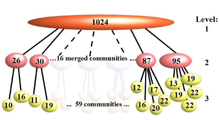
Figure 3: Heterogeneous hierarchical system corresponding to the plots in Fig. 4. In this figure, the $1024$ node system is divided into a three-level hierarchy. Level $3$ has $59$ communities with sizes from $10$ to $24$ nodes. Level $2$ has $16$ communities with sizes from $26$ to $95$ nodes. Level $1$ is the completely merged system of $1024$ nodes. The average edge density is $p=0.054$. This system has $28185$ edges.

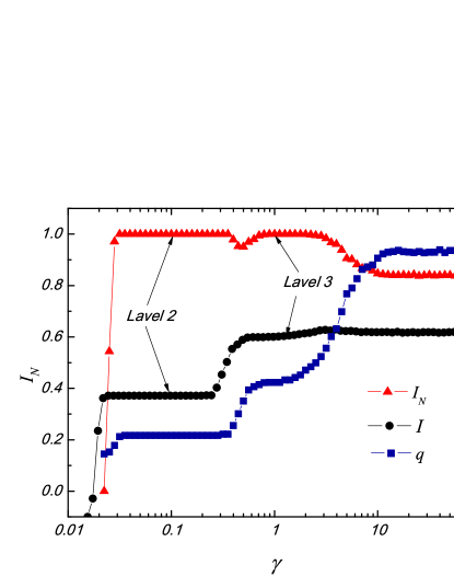
(a) Plot of information measures $I_{N}$, $I$ and the community number $q$ vs the Potts model weight $\gamma$ in Eq. (1) for the three-level heterogeneous hierarchy depicted in Fig. 3.

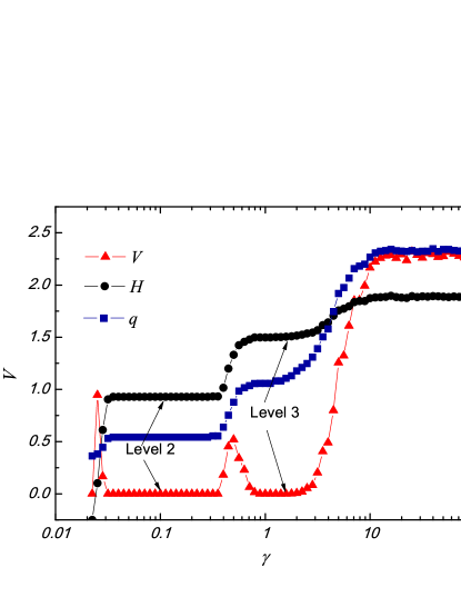
(b) Plot of information measures $V$, $H$ and the community number $q$ vs Potts model weight $\gamma$ in Eq. (1) for the three-level heterogeneous hierarchy depicted in Fig. 3. .

Figure 4: Plot of information measures $I_{N}$, $V$, $H$ and $I$ vs the Potts model weight $\gamma$ in Fig. 3. In panel(a), the peak (plateau) $I_{N}$ denoted by the arrows correspond to levels 2 and 3 of the hierarchy depicted in Fig. 3. Similarly in panel (b), the minimal $V$ values, indicated by arrows, accurately correspond to levels 2 and 3 of the hierarchy. The number of communities $q$ is $16$ and $59$ in disparate plateau regions (denoted by the arrows) in both panels. These communities assignments (and, obviously, also their numbers) are exactly the same as those of the communities in levels 2 and 3 of the original hierarchical graph of Fig. 3. In panels (a) and (b), both the mutual information $I$ and the Shannon entropy $H$ display a plateau behavior corresponding to the correct solutions.

Fig. 4 shows the result of multiresolution algorithm applied to the three-level hierarchy system in Fig. 3. The system investigated is that of a standard simple graph with unweighted links (i.e., in Eq.(1), $A_{ij}=1$ if nodes $i$ and $j$ share an edge and is zero otherwise). In Fig. 3, “level $3$” communities exhibit a density of links $p_{3}=0.9$ (i.e., a fraction $p_{3}$ of the intra-community node pairs are connected by a link ($A_{ij}=1$)). The individual communities in level $3$ have sizes that range between $5$ to $24$ nodes. The less dense communities in level $2$ harbor a density of links $p_{2}=0.3$; the nodes in this case, are divided into five groups with sizes that vary from $26$ to $95$. Highest up in the hierarchy is the trivial level $1$ “partition”- that of a completely merged system of $1024$ nodes. Thus, as a function of $\gamma$, this easily solvable system exhibits “transitions” between different stable solutions corresponding to different regions (or basins) of $\gamma$. In Sections(X, XI.7), we will further discuss additional transitions between easy solvable regions and regions of parameter space which are very “hard” or impossible (“unsolvable”).

Fig. 4(a) depicts the averages of $I_{N}$ (on the left axis) and $I$ (right axis) over all replica pairs. (We further provide in this figure the number of communities $q$.) A “cascade” composed of three plateaus is evident in these information theory measures. Similarly, Fig. 4(b) shows the $V$ in left axis and $H$ in right axis average over all replica pairs. The extrema denoted by the arrows in both panel (a) and (b) are the correctly identified levels $2$ and $3$ respectively of the hierarchy depicted in Fig. 3. The two plateaus with the peak values in panel(a) correspond to a normalized mutual information of size $I_{N}=1$ (the highest theoretically possible) and similarly the corresponding minima in panel(b) have a variation of information $V=0$ (the smallest value possible) for the same range of $\gamma$ values. These extreme values of $I_{N}$ and $V$ indicate perfect correlations among the replicas for both levels of the hierarchy. The “plateaus” in $H$, $I$ and $q$ are also important indicators of system structure. These plateau (and more general extrema elsewhere) illustrate when the system is insensitive to parameter changes and approaches stable solutions. In Section X (and in Eq.(21) in particular), we will discuss this more generally in the context of the phase diagram of the community detection problem.

VIII Replica correlations as weights in a graph

Within the multiresolution method, significant structures are identified by strongly-correlated replicas (multiple copies of the studied system). Thus, if a node pair is always in the same community in all replicas, the two nodes must have strong preference to be connected or have a large edge weight. Similarly, if a node pair is not always in the same community in all replicas, they must have preference not to be connected or have a small edge weight. We re-assign edge weights based on the correlations between replicas.

Specifically, we first generate $r$ replicas by permuting the “symmetric” initialized state of one node per cluster of the studied system, then apply our community detection algorithm to each replica and record the community membership for each node. We then calculate the probability of each node pair based on the statistics of replicas. The probability is defined as follows

$$p_{ij}=\frac{1}{r}\sum_{\alpha=1}^{r}\omega_{ij}^{\alpha},$$ (17)

where

$$\omega_{ij}^{\alpha}=\delta_{\sigma_{i}^{\alpha},\sigma_{j}^{\alpha}}+(1-\delta_{\sigma_{i}^{\alpha},\sigma_{j}^{\alpha}})\frac{\exp(-|{\bf r}_{i}^{\alpha}-{\bf r}_{j}^{\alpha}|/\ell)}{N_{A}^{\alpha}N_{B}^{\alpha}}.$$ (18)

In Eq. (18), when node $i$ and $j$ belongs to the same community in replica $\alpha$, i.e., $\delta_{\sigma_{i}^{\alpha},\sigma_{j}^{\alpha}}=1$, $\omega_{ij}^{\alpha}=1$. When node $i$ and $j$ are not in the same community in replica $\alpha$, i.e., $\delta_{\sigma_{i}^{\alpha},\sigma_{j}^{\alpha}}=0$ (we use $A$ and $B$ to represent these two different communities, where $i\in A$ and $j\in B$. $N_{A}^{\alpha}$ and $N_{B}^{\alpha}$ denote the size of cluster $A$ and $B$ in replica $\alpha$), $\omega_{ij}^{\alpha}=\frac{\exp(-|{\bf r}_{i}^{\alpha}-{\bf r}_{j}^{\alpha}|/\ell)}{N_{A}^{\alpha}N_{B}^{\alpha}}$. As throughout, $|{\bf r}_{i}^{\alpha}-{\bf r}_{j}^{\alpha}|$ is the distance between node $i$ and $j$ in replica $\alpha$. In Eq. (17), we sum the probability in each replica to define the edge weight. The assigned weights given by Eq. (17) are based on a frequency type inference. Although we will not report on it in this work, it is possible to perform Bayesian analysis with weights (“priors”) that are derived from a variant of Eq. (18); this enables an inference of the correlations from the sequence of results concerning the correlations between nodes $i$ and $j$ in a sequence of different replicas.

In unweighted graphs, we connect nodes if the edge weight between the node pair is larger than some threshold value $\bar{p}$ in Eq. (1), i.e.,

$$A_{ij}=\Theta(p_{ij}-\bar{p}).$$ (19)

In weighted graph, the analog of Eq. (2) is the Hamiltonian given by

$${\cal{H}}=\frac{1}{2}\sum_{a=1}^{q}(\bar{p}-p_{ij})\Big{[}\Theta(p_{ij}-\bar{p})+\gamma\Theta(\bar{p}-p_{ij}))\Big{]}\delta(\sigma_{i},\sigma_{j}).$$ (20)

That is, when there is a high probability $p_{ij}$, relative to a background threshold $\bar{p}$, that nodes $i$ and $j$ are linked, we assign a positive edge weight to the link $(ij)$ of size $(p_{ij}-\bar{p})$. Similarly, if the probability of a link $(ij)$ is low, we assign a negative weight of size $\gamma(p_{ij}-\bar{p})$.

Armed with Eq. (20), we then minimize in an identical fashion to the minimization of Eq. (2) that we discussed earlier. Specifically, we follow the 4 steps outlined in Section VI for non multi-scale images and the 7 steps of Section VII.2 in the analysis of general multi-scale systems.

IX Summary of parameters

We now very briefly collect and list anew the parameters that define our Hamiltonians and appear in our methods.

$\bullet$ The resolution parameter $\gamma$ in Eqs.(1, 2, 20). This parameter sets the graph scale over which we search for communities. This parameter is held fixed (typically with a value of $\gamma={\cal{O}}(1)$) in the community detection method and varies within our multi-scale analysis. We determine the optimal value of $\gamma$ by determining the local extrema of the average information theory overlaps between replicas.

$\bullet$ The spatial scale $\ell$ in Eq.(7). Similar to the more general graph scale set by $\gamma$, we may determine optimal $\ell$ by examining extrema in the average inter-replica information theory correlations. In practice, in all but the hardest cases (i.e., the case of the dalmatian dog in Fig.(1)), we ignored this scale and fixed $\ell$ to be infinite. Fixing $\ell=1$ led to good results in the analysis of the dalmatian dog.

$\bullet$ The spatial cutoff scale $\Lambda$ for defining link weights- see the brief discussions after Eqs.(6, 10). Whenever the spatial distance between two sites or blocks exceeded a threshold distance $\Lambda$ we set the link weight to be zero. We did not tune this parameter in any of the calculations. It was fixed to the value of $\Lambda=30$.

$\bullet$ The scale of the block size $L_{x,y}$ introduced in Section IV.2.1. This parameter is far smaller than the image size $N_{x}\times N_{y}$, yet large enough to cover the image features. We usually set $L_{x}\times L_{y}$ to be $9\times 9$ for an image size $N_{x}\times N_{y}$ of around $200\times 200$.

$\bullet$ The background intensities $\bar{V}$ in Eq.(2) and $\bar{p}$ in Eq.(20). Similar to the graph scale set by $\gamma$ and $\ell$, we may determine the optimal $\bar{V}$ and $\bar{p}$ by observing the local extrema of the average information correlations between replicas.

As we will elaborate on briefly, all optimal parameters can be found by determining the local extrema of the information theory correlations that signify no change in structure over variations of scale. In reality, we may fix some parameters and vary others–usually, $\Lambda$ fixed as $30$, $L_{x}\times L_{y}$ in the range of $7\times 7$ to $11\times 11$, and $\gamma$, $\bar{V}$ and $\bar{p}$ been changed.

As an aside, in this brief paragraph, we briefly note for readers inclined towards spin glass physics and optimization theory that, in principle, in the large $N$ limit (images with a large number of pixels) the effective optimal values for the likes of the parameters listed above may be derived by solving the so-called “cavity” equations mezard2 that capture the maximal inference possible (in their application without the aid of replicas that we introduced here) infer ; lenka . In the current context, in applying these equations anew to image segmentation, we arrive at the maximal inference possible of objects in an image. While these equations are tractable for simple cases, solving these equations is relatively forbidding for general cases. In practice, we thus efficiently directly examine our Potts model Hamiltonians of Eqs. (1, 2, 20) and, when needed, directly infer optimal values of the parameters by examining inter-replica correlations as described in the earlier sections. This will be expanded on in the next section (specifically, in Eq.(21)). [Detailed applications of this method are provided in Section XI.7.]

X Computational Complexity, the Phase Diagram, and the determination of optimal parameters

Our community detection algorithm is very rapid. For a system with $L$ links, the typical convergence time scales as ${\cal{O}}(L^{1.3})$ peter2 . In an image with $N$ pixels, with all of the constants $\Lambda,L_{x,y}={\cal{O}}(1)$ (i.e., not scaling with the system size), the number of links $L\sim N$.

Our general multi-scale community detection algorithm (that with varying $\gamma$) has a convergence time $\tau\sim L^{1.3}\ln N$ peter1 . Thus, generally, for an image of size $N$, the convergence time $\tau\sim N^{1.3}\ln N$. Rapid convergence occurs in all but the “hard phase” of the community detection problem.

Specifically, we numerically investigated the phase diagram as a function of noise and temperature (i.e., when different configurations are weighted with a Boltzmann factor $\exp(-\beta{\cal{H}})$ with $\beta=1/T$ at a temperature $T$ for general graphs with an arbitrary number of clusters in dandan .) Related analytic calculations were done for sparse graphs in lenka . In particular, in these and earlier works peter2 ; peter1 it was found that there is a phase transition between the detectable and undetectable clusters. The detectable phase further splinters into an “easy” and a “hard” phase. These three phases in the community detection problem constitute analogs of three related phases in the “SAT-hard-unSAT” in k-SAT problem mezard1 ; mezard2 . The found phase diagram dandan exhibits universal features. Increasing the temperature can aid the detection of clusters dandan . The universal features of the phase diagram and the known cascade of transitions that appear on introducing temperature enable better confidence in the results of the community detection algorithm. One of the central results of Ref.dandan is that the “easy” solvable phase(s) of the community detection problem which leads to correct relevant solutions (i.e., not noisy partitions of a structureless system) universally appear in a “flat” peter1 ; dandan phase(s) [see also the flat information theoretic curves in Fig. (4) and related discussion in Section(VII.2)] as ascertained by the inter-replica averages of all thermodynamic and information theoretic quantities $\{\langle Q\rangle\}$. These may correspond to the internal energy $(Q={\cal{H}})$, average Shannon entropy ($Q=H$), average inter-replica normalized mutual information and variation of information ($Q=I_{N},V$), the complexity $(Q=\Sigma)$ mezard2 or an associated “susceptibility” $(Q=\chi)$ peter1 ; dandan that monitors the onset of large complexity. [This susceptibility will be defined with the aid in the change in the average normalized mutual information $I_{N}$ as a function of the number of trials $t$. It is defined as $\chi(n)=[I_{N}(t=n)-I_{N}(t=4)]$.] That is, with $z$ denoting a set of generalized parameters (e.g., artificially added additional noise in networks $(z=p_{out})$ dandan , temperature $(z=T)$ dandan , or resolution parameter $(z=\gamma)$ peter1 ), pertinent partitions appear for those values of the parameters $z$ for which

$$\frac{\partial\langle Q\rangle}{\partial z}=0.$$ (21)

As alluded to above, a particular realization of Eq.(21) appears in the hierarchal system discussed in Section VII.2 wherein $z=\gamma$ and $Q=I_{N},V$. In that case, Eq.(21) was satisfied in well defined plateaus.

When present, crisp solutions are furthermore generally characterized by relatively high values of $I_{N}$, and these correspond to the “easy phase” of the image segmentation problem. In Sec. XI.7, we will provide explicit analysis of the phase diagram and optimal parameters as they pertain to several example images.

All of the results (except the ones in Sec. XI.7) presented below in the current manuscript were attained at zero temperature and may be improved by the incorporation of thermal annealing as the results of dandan illustrate for general systems.

XI Results

XI.1 Brain Image

XI.1.1 Unweighted graphs

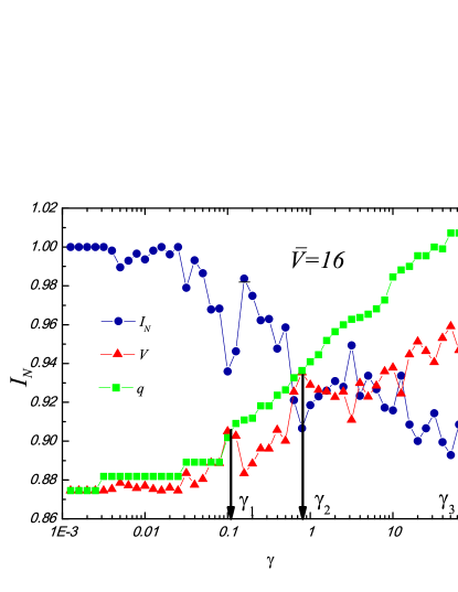
(a) The result of the “multiresolution” algorithm applied to the unweighted brain image shown in (b): $I_{N}$, $V$ and $q$ in terms of the resolution $\gamma$.

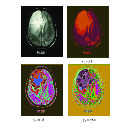
(b) The unweighted result of the brain images with different $\gamma$, which correspond to $\gamma_{1}=0.1$, $\gamma_{2}=0.8$, $\gamma_{3}=79.4$.

Figure 5: [Color Online.] The plot of the normalized mutual information $I_{N}$, variation of information $V$ and the number of communities $q$ as a function of $\gamma$ for the brain image. This image is reproduced with permission from the Iowa Neuroradiology Library. The axis for $\gamma$ is on a logarithmic scale. There are three prominent peaks in the $V$ curve. We apply our community detection algorithm to the grey-scale brain image at these three values of $\gamma$s. The corresponding results are shown in panel (b). Note that the results show three-level hierarchy as $\gamma$ varies.

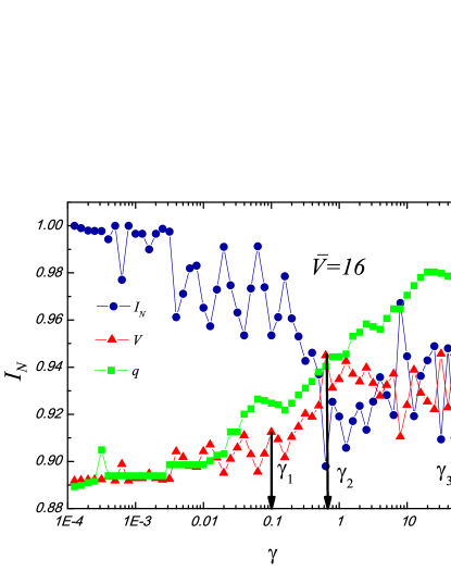
(a) The result of “multiresolution” algorithm for the weighted brain image shown in (b): $I_{N}$, $V$ and $q$ in terms of the resolution $\gamma$.

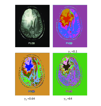
(b) The weighted result of the brain images with different $\gamma$, which correspond to $\gamma_{1}=0.1$, $\gamma_{2}=0.64$, $\gamma_{3}=64$.

Figure 6: [Color Online.] The result of “multiresolution” for the weighted brain image shown in panel (b). In panel (a), the “multiresolution” result here behaves different from Fig. 5 but keeps the same trend. The structure is only stable in the resolution range of $\gamma<0.01$, compared to the wider range of $\gamma<0.1$ in Fig. 5. This illustrates that the weighted graph is more sensitive to the change of resolution.

We start the review of the results of our methods by analyzing an unweighted graph (Eq. (1)) for the grey-scale brain image as shown in Fig. 5. We will assign edges between pixels only if the intensity difference is less than the threshold $\bar{V}=16$ as denoted in panel (a) of Fig. 5. The algorithm uses Eq. (1) to solve for a range of resolution parameters $\gamma$ in the interval $[\gamma_{0},\gamma_{f}]$. In the particular case in Fig. 5, $\gamma_{0}=10^{-3}$ and $\gamma_{f}=100$. There are two more input parameters that are needed in our algorithm: the number of independent replicas $r$ that will be solved at each tested resolution and the number of trials per replica $t$. We use $r=10$ and $t=4$ in Fig. 5 respectively.

As noted earlier (see Section V), for each replica, we select the lowest energy solution among the $t$ trials. The $r$ replicas are generated by reordering the “symmetric” initialized state of one node per community. We then use the information based measures (i.e., $I_{N}$ or $V$) to determine the multiresolution structure.

The plots of $I_{N}$, $V$ and $q$ as a function of $\gamma$ in Fig. 5 exhibit non-trivial behaviors. Extrema in $I_{N}$ and $V$ correspond to jumps in the number of communities $q$. In the low $\gamma$ region, i.e., $\gamma<0.1$, the number of communities is stable. However, when $\gamma>0.1$, the number of communities $q$ sharply increase. This indicates that the structure changes rapidly as the resolution $\gamma$ varies. There are three prominent peaks in the $V$ (variation of information) curve. We show the corresponding images at these resolutions, that is in panel(b) in Fig. 5. These corresponding segmented images show more and more sophisticated structures. The lower right image at a resolution of $\gamma=79.4$ shows the information in detail. Different colors in the image correspond to different clusters. There are, at least, five contours surrounding the tumor, that denote the degree by which the tissue was pushed by the tumor. The lower left image at the resolution $\gamma=0.8$ is less detailed than the one on the right. Nevertheless, it retains the details surrounding the tumor. If we further decrease $\gamma$, the upper right image at the resolution $\gamma=0.1$ will not keep the details of the tumor boundary, only the rough location of the tumor. Thus, neither too large nor too small resolutions are appropriate for tumor detection in this image. The resolution around $\gamma=0.8$ is the most suitable in this case. This is in accord with our general found maxim in Section IX concerning a value of $\gamma=1$. We re-iterate that, in general, the optimal value of $\gamma$ is found by Eq.(21) (an example of which is manifest in the information theory plateaus discussed in Section VII.2). In Section XI.7, we will discuss, in depth, how the optimal values of $\gamma$ may be determined in (weighted) example systems.

XI.1.2 Weighted graphs

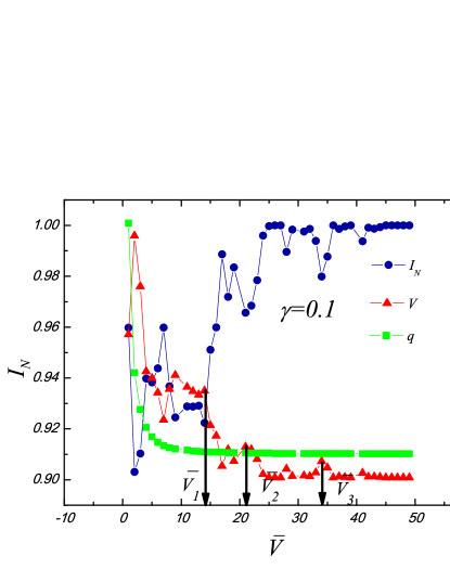
(a) The result of “multiresolution” algorithm for the weighted brain image shown in (b): $I_{N}$, $V$ and $q$ in terms of the threshold $\bar{V}$.

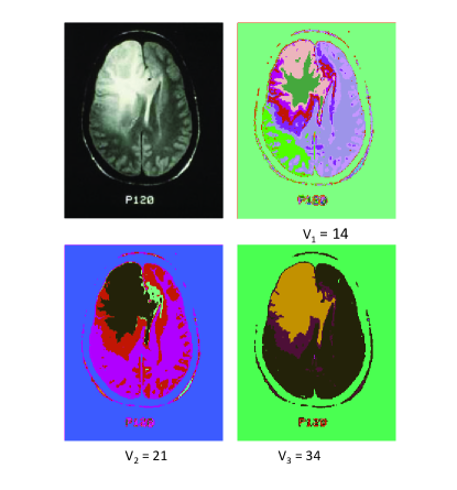
(b) The weighted result of the images with different $\bar{V}$, which correspond to $\bar{V}_{1}=14$, $\bar{V}_{2}=21$, $\bar{V}_{3}=34$.

Figure 7: [Color Online.] The “multiresolution” result also shows the hierarchy structure as the threshold $\bar{V}$ varies, as in Fig. 6. Higher “$\bar{V}$” corresponds to the lower ”$\gamma$”, which means pixels intend to merge in higher “$\bar{V}$”. The structure is stable in the range of $\bar{V}>25$, below which the structure is sensitive.

In Figs. (6, 7), we provide the “multiresolution” results for the weighted graph (Eq. (2)) of $\gamma$ and $\bar{V}$ for the brain image. Both the resolution $\gamma$ and the threshold $\bar{V}$ control the hierarchy structures: the peaks in the normalized mutual information $I_{N}$ and variation of information $V$ always correspond to the jumps in the number of communities $q$. The jumps in $q$ correlate with the changes in hierarchal structures on different scales. We can combine both parameters to obtain the desirable results in the test images. See, e.g., the $3D$ plot of $I_{N}(\bar{V},\gamma)$.

The results of our method with weighted edges are more sensitive to the changes of parameters (as seen from a comparison of Fig. 6 with Fig. 5). According to Eq. (2), edges $(ij)$ with small (or large) difference $|D_{ij}|$ will decrease (or increase) the energy by $|\bar{V}-D_{ij}|$ (or $\gamma|\bar{V}-D_{ij}|$). However, if the unweighted graphs and the Potts model with discrete weights (Eq. (1)) are applied, the edges with small or large “color” difference will decrease or increase the energy by the amount of $1$ or $\gamma$. Thus, considerable information (e.g., the “color” of each pixel) is omitted when using an unweighted graph approach.

XI.2 A painting by Salvador Dali

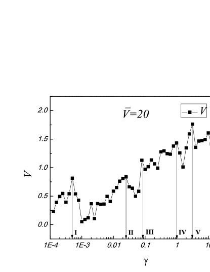
(a) The variation of information $V$ as a function of resolution $\gamma$ for the image shown in Panel(b) .

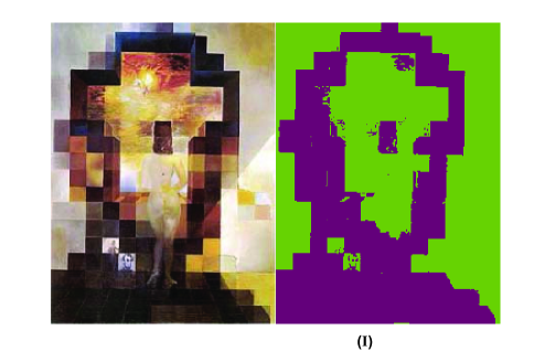
(b) The original image and the corresponding segmentation for the specific resolution marked (I) in panel(a).

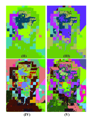
(c) The corresponding images in the specific resolution marked (II),(III),(IV) and (V) in panel(a).

Figure 8: [Color Online.] The specific image is from lincoln . At close distance, this is “Gala contemplating the Mediterranean sea” while at larger distance is “a portrait of Abraham Lincoln”. Panel(a) shows the variation of information as a function of resolution. We pick the resolution at each “peak” position and apply our algorithm at these particular resolutions. Panels (b) and (c) show the resulted images at the corresponding resolutions marked in panel (a). Note that at low resolution, the resulting segmentation clearly depicts “the portrait of Abraham Lincoln” as shown in panel (b) on the right. In particular, notwithstanding noise, as $\gamma$ increases, the segmentation results show more details and we could detect the lady in the middle in (II)-(V) of Panel(c).

We next apply our multiresolution community detection algorithm to the images that are by construction truly multi-scale. The results at different resolutions are shown in Fig. 8. The original image is that of Salvador Dali’s famous painting “Gala contemplating the Mediterranean sea which at twenty meters becomes a portrait of Abraham Lincoln”. Our algorithm perfectly detected the portrait of Lincoln at low resolution as shown in Fig. 8 in the segmentation result appearing in panel (I) of (b). As the resolution parameter $\gamma$ increases, the algorithm is able to detect more details. However, due to the non-uniform color and the similarity of the surrounding colors to those of the targets, the results are very noisy. At the threshold of $\bar{V}=20$, the algorithm has difficulty in merging pixels to reproduce the lady in the image. For example, in image (II) in Panel (c), the lady’s legs are merged into the background. In image (III), only one leg is detected. In images (IV) and (V), both legs can be detected but belong to different clusters.

XI.3 Benchmarks

In order to assess the success of our method and ascertain general features, we applied it to standard benchmarks. In particular, we examined two known benchmarks: (i) The Berkeley image segmentation benchmark and (ii) that of Microsoft Research.

XI.3.1 Berkeley Image Segmentation Benchmark

We were able to accurately detect the targets in test images, as in Figs.(9, 10). The original images in Fig. 9 were downloaded from the Berkeley image segmentation benchmark BSDS300 berkeley-paper , and those of Fig. 10 are downloaded from the Microsoft Research microsoft . We will now compare our results with the results by other algorithms. The Berkeley image segmentation benchmark provides the platform to compare the boundary detection algorithms by an “F-measure”. This quantity is defined as

$$\mbox{F-measure}=\frac{\mbox{2 }\times\mbox{Precision }\times\mbox{ Recall}}{\mbox{Precision+Recall}}.$$ (22)

“Recall” is computed as the fraction of correct instances among all instances that actually belong to the relevant subset, while “Precision” is the fraction of correct instances among those that the algorithm believes to belong to the relevant subset. Thus, we have to draw the boundaries in our results and compute the F-measure. We use the tool “EdgeDetect” of Mathematica software to draw the boundaries within our region detection results, as shown in the right column in Fig. 9. The comparison of the “F-measure” of our algorithm (“F-Absolute Potts Model”) and the best algorithm in the benchmark (“F-Global Probability of boundary”)gPb1 ; gPb2 is shown in Table. 1. On the whole, our results are better than the algorithm of the Berkeley group.

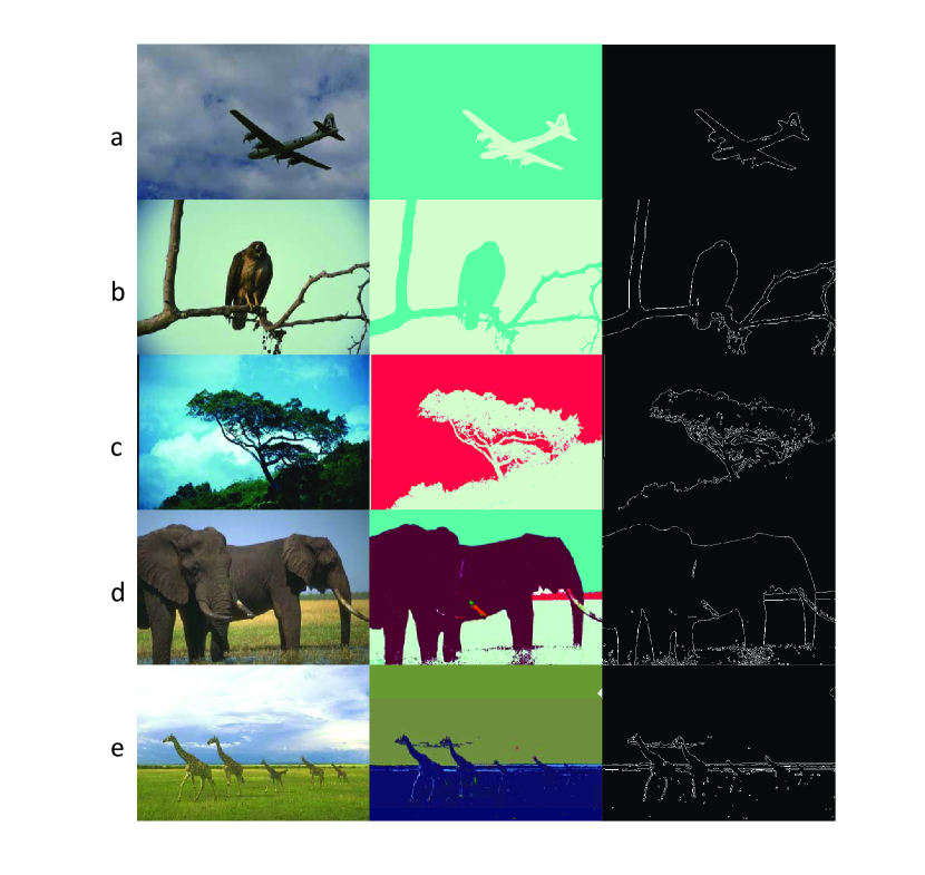
Figure 9: [Color Online.] Image segmentation results of our algorithm when tested with examples from the Berkeley BSDS300 benchmark. Shown, in the left column, are the original images. The central column contains the results of our method. The right column provides the boundaries of the images in the middle by running “EdgeDetect” of Mathematica on the results of our run in the central column. The parameters of community detection algorithm used for these images are: in (a), $\gamma=0.001$, $\bar{V}=15$. In panel (b), $\gamma=0.0001$, $\bar{V}=20$. In (c), $\gamma=0.001$, $\bar{V}=20$. In (d), $\gamma=0.01$, $\bar{V}=15$. In (e), $\gamma=0.01$, $\bar{V}=15$. We performed the boundary detection on the results of our community detection algorithm (i.e., the central column) and employed the “F-measure” accuracy parameter in order to compare the results of our algorithm with earlier results reported for the Berkeley image segmentation benchmark (shown in Table. 1).

	F-Absolute Potts Model	F-Global Probability of boundary
a	0.79	0.78
b	0.94	0.91
c	0.82	0.74
d	0.79	0.83
e	0.75	0.60

Table 1: The comparison of “F measure” for Fig. 9 by our community detection algorithm (“F-Absolute Potts Model”) with the algorithm “Global Probability of boundary” (“gPb”) gPb1 ; gPb2 which has the highest score in the Berkeley image segmentation benchmark (“F-Global Probability of boundary”). The higher F-value corresponds to the better detection. Note that our algorithm is performing better than the “gPb algorithm” in almost all images except the fourth one. Our fourth (d) image gets lower score is mostly because there are dots in the lower grass place. These small dots will lead to small high accuracy features. These features are unexpected in the ground truth and thus lower the F-value.

XI.3.2 Microsoft Research Benchmarks

In Fig. 10, we compare our results (in the rightmost column) with the ground truths provided by Microsoft Research (the central column). By adjusting the $\gamma$ and $\bar{V}$ values, we can merge the background pixels and highlight the target. In the segmentation of the image of the flower in the first row, $\gamma=0.001$ and $\bar{V}=20$. For both the picnic table in the middle row and that of the two sheep in the bottom row, we set $\gamma=0.01$ and $\bar{V}=15$.

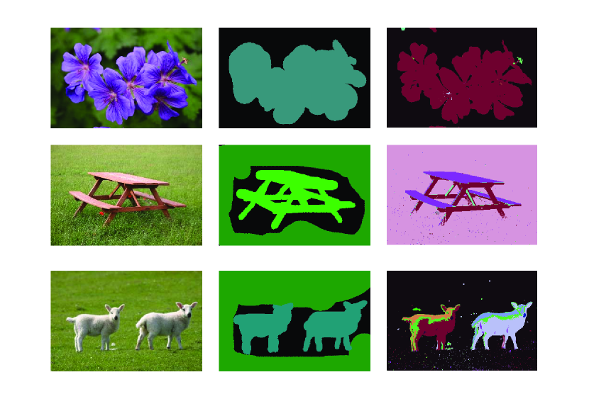
Figure 10: [Color Online.] The results of some image segmentations by our Potts model (Eq. (2)) and community detection algorithm (peter1 ). The images are downloaded from the website of Microsoft Research (microsoft ). The left column are the original images. The central column are the ground truths defined by the website of Microsoft Research (microsoft ), which are the desirable image segmentation results. The right column are the segmentation results by our algorithm. The parameters used for each image are: (1)$\gamma=0.001$, $\bar{V}=20$ for the flower image. (2) $\gamma=0.01$, $\bar{V}=15$ for the image of the picnic table. (3) Similarly, $\gamma=0.01$, $\bar{V}=15$ for the image of the two sheep. Note that our algorithm works very well for this kind of images in which the color is nearly uniform within each object.

XI.4 Detection of quasi-periodic structure in quasicrystals

Quasicrystals quasicrystal are ordered but not periodic (hence the name “quasi”). In Fig. 11, the image in row (a) is such a quasi-crystal formed by “Penrose tiling”. We applied the Fourier transform method to reveal the corresponding underlying structures. In row (a), the image marked by (I) is the original image (downloaded from quasi1 ), the one with notation (II) is the result of our algorithm, and (III) is the image of (II) with the connections of the nearest neighbor nodes. The images marked by (II) and (III) show the first Penrose tiling (tiling P1). Penrose’s first tiling employs a five-pointed pentagram, 3/5 pentagram shape and a thin rhombus. Similarly, the result images of panels (II) and (III) in row (b) reveal the underlying structure of the superlattice with $AB_{4}$ stoichiometry and the structural motif of the ($3^{2}.4.3.4$) “Archimedean tiling” of the original image (I) (from quasi2 ). The Archimedean tiling displayed in image (III) of row (b) of Fig. 11 employs squares and triangles. It is straightforward to analyze the quasi-periodic structure by applying our image segmentation algorithm as shown in Fig. 11. By iterating the scheme outlined herein, structure on larger and larger scales was revealed.

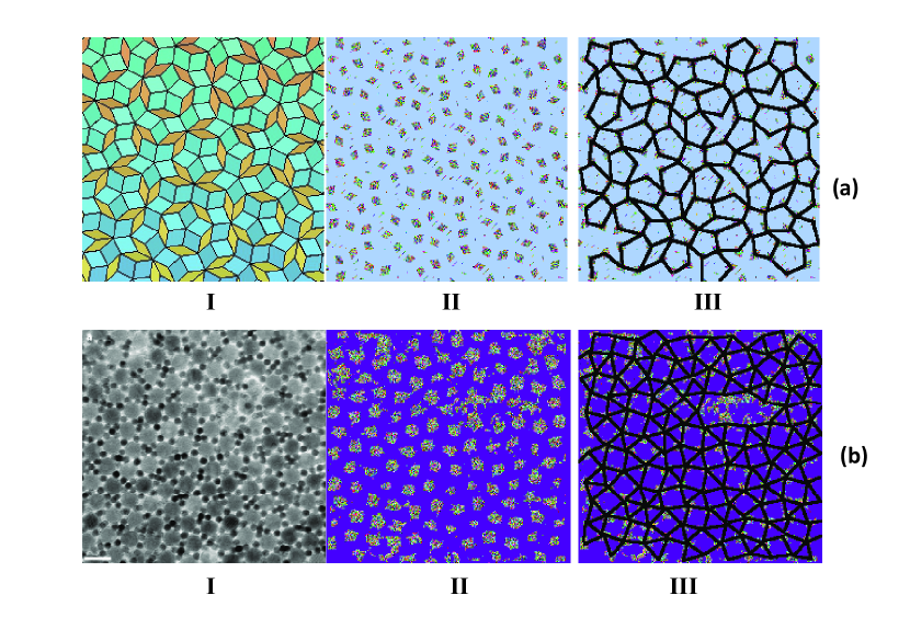
Figure 11: [Color Online.] Quasicrystal images are displayed in panels (I). The corresponding image segmentation results by our algorithm are shown in (II). In (III), we connect the basic object by line, resulting in large basic blocks. This process can be repeated recursively leading to larger and larger scale structures. Note that we are able to reveal the underlying quasi-periodic structures in both row (a) (the original image in (I) is from quasi1 ) and (b) (the original image in (I) is from quasi2 ). We show the first Penrose tiling (tiling “P1”) in (a), and the structural motif of the ($3^{2}.4.3.4$) Archimedean tiling in (b).

XI.5 Images with spatially varying intensities

If the target is similar to the background (as in, e.g., animal camouflage), then the simplest initialization of edges with linear weights will, generally, not suffice. For example, in Fig. 12 the zebra appears with black and white stripes. It is hard to directly detect the stripes of the zebra because of the large “color” difference between the black and white stripes of the zebra. Fig. 14 has the similar stripe-shaped background which is very difficult to distinguish from the zebra itself by using the weights of Eqs.(7, 8) for the edges. Towards this end, we will next employ the Fourier transform method of Sec. IV.2.3.

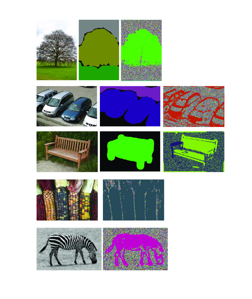
Figure 12: [Color Online.] The image segmentation results by the community detection algorithm with Fourier weights as described in Section IV.2.3. Some of the images are downloaded from the Microsoft Research (microsoft ) and some of them are download from the Berkeley image segmentation benchmark (berkeley-paper ). The left column contains the original images. The central column (apart from the last two rows) provides the “ground truths”. The right images on the right are our results. The parameters used in each image are: (1) $\gamma=0.01$, $\bar{V}=-300$ for the tree image. (2) $\gamma=0.1$ and $\bar{V}=-300$ for the car image. (3) $\gamma=0.01$ and $\bar{V}=-400$ for the bench image. (4) $\gamma=0.01$, $\bar{V}=-100$ for the image of corn. (5) $\gamma=0.1$, $\bar{V}=-900$ for the zebra image. Even though the color is not uniform inside the targets, we can nevertheless easily detect the targets by this method.

As seen in Fig. 12, the original images are not uniform. Rather, these images are composed of different basic components such as stripes or spots, etc. With the aid of Fourier transform within each block, as discussed in Section IV.2.3, we are able to detect the target. For some of the images such as the second one in Fig. 12, when the target is composed of more than one uniform color or style, our community detection algorithm is able to detect the boundaries, but the regions inside the boundary are hard to merge. This is because the block size is smaller than that needed to cover both the target and the background. That is, block size of $L_{x}\times L_{y}=5\times 5$ is much smaller than the image size of $N_{x}\times N_{y}=320\times 213$ in the car image in the second row, so most of the blocks are within one color of the target (car) or the background (ground). However, the dominant Fourier wave-vector of the region within one color component of the car is similar to that of the ground. Therefore, the algorithm always treats them as the same cluster, rather than merging the region inside the car with the boundary.

In other instances (e.g., all the other rows except the second in Fig. 12), the targets are markedly different from the backgrounds. Following the scheme discussed in Section X (that will be fleshed out in Section XI.7), we may always optimize parameters such as the resolution, threshold, or the block size to obtain better segmentation.

XI.6 Detection of camouflaged objects

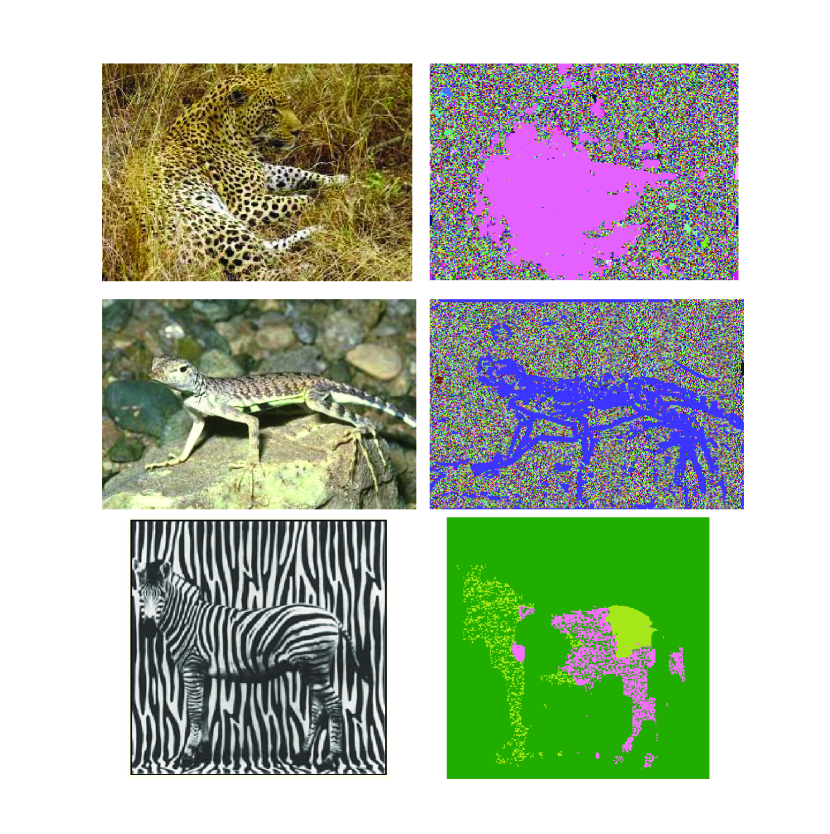
Figure 13: [Color Online.] The results of the image segmentation for a “camouflaged image”. The image of the leopard is from (wikipedia ), the lizard is provided in the Berkeley image segmentation benchmark(berkeley-paper ), and the last image is from the website of the EECS department of Berkeley (berkeley-zebra ). The parameters for the shown segmentations are: (1) $\gamma=1$, $\bar{V}=-700$ for the image of the leopard, (2) $\gamma=0.1$, $\bar{V}=-500$ in the image of the lizard, and (3) $\gamma=1$, $\bar{V}=-1100$ for the zebra image.

(a) The variation of information $V$ as a function of the negative threshold $-\bar{V}$ for the zebra image in panel (b).

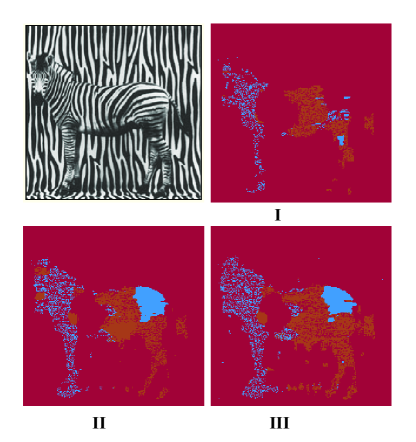
(b) The weighted results of the zebra images at the corresponding thresholds: $\bar{V}_{1}=-760$ (I), $\bar{V}_{2}=-1040$ (II), and $\bar{V}_{3}=-1200$ (III).

Figure 14: [Color Online.] The “multiresolution” result of zebra with fixed community number $q=3$ and resolution $\gamma=1$. In panel(a), we plot the variation of information $V$ as a function of negative threshold $-\bar{V}$. The peaks in $V$ correspond to the changes of structures. We choose three peaks and run the algorithm at these three particular thresholds, and the result images are shown in panel (b). As $|\bar{V}|$ increases, less regions in the zebra merge to the background, and the boundary becomes more clear. If we increase the threshold further, the result is more noisy as the last image of $\bar{V}=-1200$ (III) shows.

In the images of Fig. 12, the target objects are very different from their background. However, there are images wherein (camouflaged) objects are similar to their background. In what follows, we will report on the results of our community detection algorithm when these challenging images were analyzed. In all of the cases below in Section XI.6.1, the edge weights were initialized by the Fourier amplitudes discussed earlier (Section IV.2.3). In the case of the dalmatian dog image in Section XI.6.2, we further employed the method of average intensity difference between blocks discussed in Section IV.2.2. In all cases but this last one of the dalmatian dog, we fixed the length scale parameter $\ell$ of Section IV.2.3 to be infinite.

XI.6.1 Images of a leopard, a lizard, and a zebra

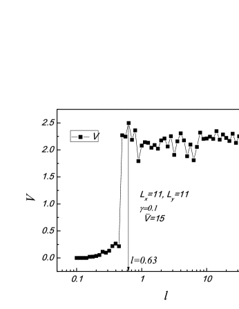
(a) The variation of information $V$ as a function of length $\ell$ at $\gamma=0.1$

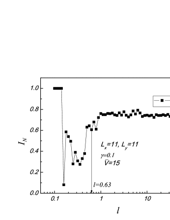
(b) The normalized mutual information $I_{N}$ as a function of length $\ell$ at $\gamma=0.1$

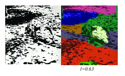
(c) The corresponding image segmentation result at the extremum of $V$/$I_{N}$ in panel (a)/(b)

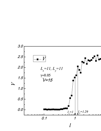
(d) The variation of information $V$ as a function of length $\ell$ at $\gamma=0.05$

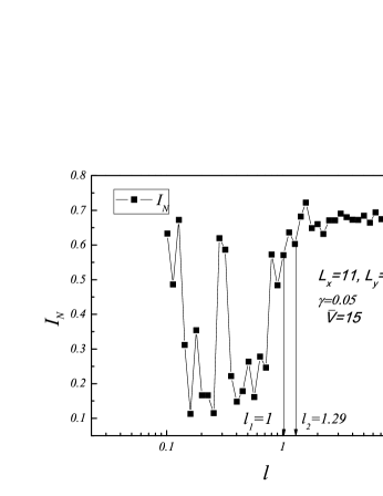
(e) The normalized mutual information $I_{N}$ as a function of length $\ell$ at $\gamma=0.05$

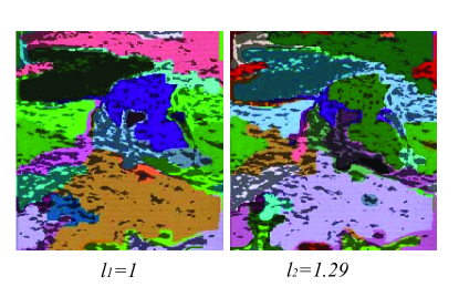
(f) The corresponding image segmentation results at the extremum, and at a point close to the peak of $V$/$I_{N}$ in panel (d)/(e).

Figure 15: [Color Online.] Results of our algorithm as a function of the length scale $\ell$ in Eq. (7) for the dalmatian dog image. Plots of the variation of information and the normalized mutual information ($V$, $I_{N}$) as a function of the length scale $\ell$ appear in panels (a, b)(at resolution of $\gamma=0.1$) and (d, e) ($\gamma=0.05$ ). Panel (c) shows the original image. As seen in panels (a,b), a coincident local maximum of $V$ and local minimum of $I_{N}$ appears (for $\gamma=0.1$) at $\ell=0.63$. Similarly, panel (f) shows the images corresponding to the peak of $V$ (coincident with a local minimum of $I_{N})$ in panel (d) (and (e)) at $\ell_{2}=1.29$ (and $\gamma=0.05$). We examine the results for $\ell_{1}=1$ in panel (f). We are able to detect the body and the back two legs of the dog, even though with some “bleeding” in panel (f). In (c), we are detecting well except for the inclusion of some “shade” noise under the body.

“Camouflage” refers to a method of hiding. It allows for an otherwise visible organism or object to remain unnoticed by blending with its environment. The leopard in the first row of Fig. 13 is color camouflaged. With our algorithm, we are able to detect most parts of the leopard except the head. The lizard in the second row uses not only the color camouflage but also the style camouflage, both the lizard and the ground are composed of grey spots. We can detect the lizard. The zebra in the bottom row uses the camouflage– both the background and the zebra have black-and-white stripes. Our result is very accurate, even though the algorithm treats the middle portion of the zebra (the position of the “hole”) as the background by mistake. This is because, in this region, the stripes within the zebra are very hard to distinguish from the stripes in the background, they are both regular and vertical.

We applied the “multiresolution” algorithm to the zebra image in the last row of Fig. 13 as shown in Fig. 14. The number of communities is $q=3$, the resolution parameter $\gamma=1$ and the threshold $\bar{V}$ was varied from $\bar{V}=-600$ to $\bar{V}=-1800$. In the low $|\bar{V}|$ area, some regions inside the zebra tend to merge into the background (the image with the threshold $\bar{V}=-760$). As the background threshold $|\bar{V}|$ increases in magnitude, the boundary of the zebra becomes sharper (the shown segmentation corresponds to a threshold of $\bar{V}=-1040$). For yet larger values of $|\bar{V}|$, the results are noisy (the image with the threshold $\bar{V}=-1200$). Thus, in the range $760\leq|\bar{V}|\leq 1200$, we obtain the clear detection seen in the last row of Fig. 13.

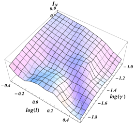
(a) A 3d plot of the normalized mutual information $I_{N}$ as a function of $\log(\ell)$ and $\log(\gamma)$.

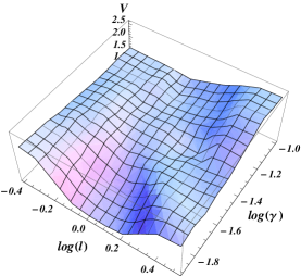
(b) The 3d plot of the variation of information $V$ as the function of $\log(\ell)$ and $\log(\gamma)$

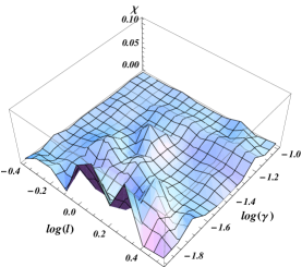
(c) Plots of the susceptibility $\chi$ as the function of $\log(\ell)$ and $\log(\gamma)$

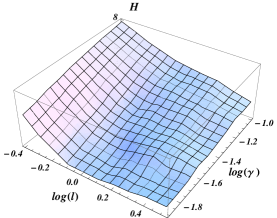
(d) The Shannon entropy $H$ as a function of $\log(\ell)$ and $\log(\gamma)$.

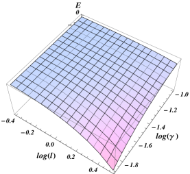
(e) The energy $E$ as a function of $\log(\ell)$ and $\log(\gamma)$.

Figure 16: Plots of $I_{N}$, $V$, $\chi$, $H$ and energy $E$ as the function of $\log(\ell)$ and $\log(\gamma)$ for the “dalmatian dog” image in Fig. 15.

XI.6.2 Dalmatian dog

The camouflaged dalmatian dog in panel (c) of Fig. 15 (and Fig. 1) is a particularly challenging image. We invoke the method detailed in Sec. IV.2.2 to assign edge weights. We then apply the multiresolution algorithm to ascertain the length scale $\ell$ in Eq. (7). The inter-replica averages of the variation of information $V$ and the normalized mutual information $I_{N}$ are, respectively, shown in panels (a,b) and panels (d,e) of Fig. 15. These information theory overlaps indicate that, as a function of $\ell$, there are, broadly, two different regimes separated by a transition at $\ell\sim 1$. We determine the value of $\ell$ at the local information theory extremum that is proximate to this transition and determine the edge weights set by this value of $\ell$. (See Eq. (7).) In Section XI.7.1, we will illustrate how we may determine an optimal value of $\ell$.

We segment the original image of the dalmatian dog via our community detection algorithm as shown in panels (c) and (f) in Fig. 15. The result in panel (c) corresponds to a resolution of $\gamma=0.1$. The image on the right in panel (c) is the superimposed image of our result and the original image (on the left) at the particular length $\ell=0.63$. The “green” color corresponds to the dalmatian dog. The method is able to detect almost all the parts of the dog except the inclusion of “shade” noise under the body. The results in panel (f) correspond to a resolution $\gamma=0.05$. The image on the left in panel (f) is the superimposed image of our immediate running result and the original one at the length $\ell_{1}=1$, which is close to the maximum of $V$ (and the local minimum of $I_{N}$). On the right, we provide the result for $\ell_{2}=1.29$ (a value of $\ell$ corresponding to a maximum of $V$ and a minimum of $I_{N}$). The “purple” color in the segmented image corresponds to the dalmatian dog. We are able to detect the body and the two legs in the back, even though with some “bleeding”. As we will discuss in the next subsection, it is possible to relate the contending solutions found in Fig.(15) for different values of $\gamma$ and $\ell$ to the character of the phase diagram.

XI.7 Phase Diagram

As previously alluded to in Sec. X, we investigated numerically the phase diagram and the character of the transitions of the community detection problem for general graphs in dandan . From this, we were able to distinguish between the “easy”, “hard” and “unsolvable” phases as well as additional transitions within contending solutions within these phases (e.g., our discussion in Section VII.2). Strictly speaking, of course, different phases appear only in the thermodynamic limit of a large number of nodes (i.e., $N\to\infty$). Nevertheless, for large enough systems ($N\gg 1$), different phases are, essentially, manifest. As we will now illustrate, the analysis of the phase diagram enables the determination of the optimal parameters for the image segmentation problem. To make this connection lucid, we will, in this section, detail the phase diagrams of several of the images that we analyzed thus far.

XI.7.1 Phase diagram of the Potts model corresponding to the dalmatian dog image

We will now analyze the thermodynamic and information theory measures as they pertain to the dalmatian dog image (Fig. 15) for a range of parameters. In a disparate analysis, in subsection XI.7.2, we will extend this approach also to finite temperature (i.e., $T>0$) where a heat bath algorithm was employed. Here, we will content ourselves with the study of the zero temperature case that we have focused on thus far.

Plots of the normalized mutual information $I_{N}$, variation of information $V$, susceptibility $\chi$, entropy $H$, and the energy $E$ are displayed in Fig. 16. We set the background intensity to $\bar{V}=15$. The block size is $L_{x}\times L_{y}=11\times 11$. We then varied the resolution $\gamma$ and the spatial scale $\ell$ within a domain given by $\gamma\in[0.01,0.1]$ and $\ell\in[0.4,4]$. In Fig. 16, all logarithms are in the common basis (i.e., $\log_{10}$).

Several local extrema are manifest in Fig. 16. In the context of the data to be presented below, the quantity $Q$ of Eq. (21) can be $I_{N}$, $V$, $\chi$, $H$ or $E$, and $z$ may be $\gamma$ or $\ell$. Examining the squares of the gradients of these quantities, as depicted in Fig. 17, aids the identification of more sharply defined extrema and broad regions of the parameter space that correspond to different phases.

In Fig. 17, we compute the squares of the gradients of $I_{N}$, $V$, $\chi$, $H$ and $E$ in panels (a) through (e). Panel (f) shows the sum of the squares of the gradients of $I_{N}$, $V$ and $\chi$. A red dot denotes parameters for a “good” image segmentation with the parameter pair being $(\gamma,\ell)=(0.05,1)$ (or $(\log(\gamma),\log(\ell))=(-1.3,0)$ corresponding to the left hand segmentation in panel (f) of Fig. 15). Clearly, the red dot is located at the local minimum in each panel. This establishes the correspondence between the optimal parameters and the general structure of the information theoretic and thermodynamic quantities.

As evinced in Fig. 17, there is a local single minimum which is surrounded by several peaks in the 3D plots of the squares of the gradients of $I_{N}$, $V$ (panel(a),(b)) and their sum (panel (f)). For the dalmatian dog image (Fig. 15, setting $Q$ in Eq. (21) to be the square of the gradients efficiently locates optimal parameters. Note that the other contending solutions in Fig. (15) relate naturally to the one at $\gamma=0.05$ and $\ell=1$. The $\ell=1.29$ (i.e., $\log(\ell)=0.11$) solution on the right hand side of panel (f) appears in the same “basin” as that of the $\ell=1$ solution. Indeed, both segmentations of panel (f) of Fig. (15) share similar features. By contrast, the $\gamma=0.1$ and $\ell=0.63$ (i.e., ($\log(\gamma)=-1,\log(\ell)=-0.2$)) segmentation result of panel (c) in Fig.(15) relates to a different region.

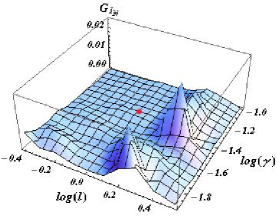
(a) The square of the gradient of $I_{N}$ (panel (a) of Fig. 16) as a function of $\log(\ell)$ and $\log(\gamma)$.

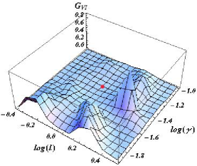
(b) The square of the gradient of $V$ (panel (b) of Fig. 16) as a function of $\log(\ell)$ and $\log(\gamma)$.

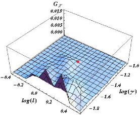
(c) The square of the gradient of $\chi$ (panel(c) of Fig. 16) as a function of $\log(\ell)$ and $\log(\gamma)$.

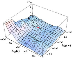
(d) The square of the gradient of $H$ (panel (d) of Fig. 16) as the function of $\log(\ell)$ and $\log(\gamma)$.

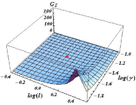
(e) The square of the gradient of $E$ (panel (e) of Fig. 16) as the function of $\log(\ell)$ and $\log(\gamma)$.

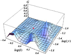
(f) The sum of the squares of the gradients of $I_{N}$, $V$ and $\chi$ (panel (a),(b) and (c) of Fig. 16) as the function of $\log(\ell)$ and $\log(\gamma)$.

Figure 17: Information theory and thermodynamic measures relating to the dalmatian dog image of Fig. 15. The squares of the gradient of $I_{N}$, $V$, $\chi$, $H$, $E$ (panel (a)-(e)) and the sum of the squares of the gradients of $I_{N}$, $V$ and $\chi$ (panel (f)) as the function of $\log(\ell)$ and $\log(\gamma)$. The red dot in each panel denotes the location of the parameters ($(\log(\ell)$,$\log(\gamma))=(0,-1.3)$ (i.e., $(\ell,\gamma=(1,0.05)$) of the results in Fig. 15. This good segmentation found for these parameters correlates with a local minimum within each panel.

XI.7.2 A finite temperature phase diagram

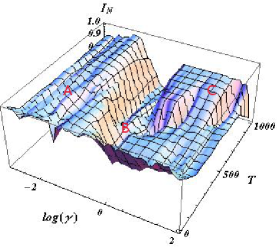
(a) The normalized mutual information $I_{N}$ as a function of the resolution $\log(\gamma)$ and temperature $T$.

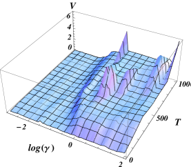
(b) The variation of information $V$ as the function of the resolution $\log(\gamma)$ and temperature $T$.

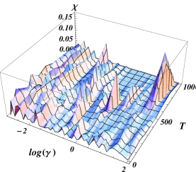
(c) The susceptibility $\chi$ as the function of the resolution $\log(\gamma)$ and temperature $T$.

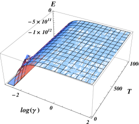
(d) The energy $E$ as a function of the resolution $\log(\gamma)$ and temperature $T$.

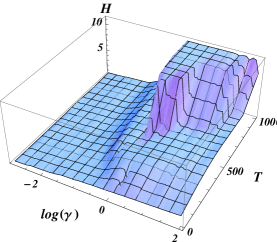
(e) The Shannon entropy $H$ as the function of the resolution $\log(\gamma)$ and temperature $T$.

Figure 18: The normalized mutual information $I_{N}$, variation of information $V$, susceptibility $\chi$, energy $E$ and Shannon entropy $H$ as the function of the resolution $\log(\gamma)$ and temperature $T$ for the “bird” image in Fig. 19. In panel (a), we mark (i) the “easy” phase (where $I_{N}$ is almost $1$) as “A”, (ii) the “hard” phase (where $I_{N}$ decreases) by “B”, and (iii) denote the “unsolvable” phase (where $I_{N}$ forms a plateau whose value is less than $1$) by “C”. The physical character of the “easy”, “hard”, and “unsolvable” phases is further evinced by the corresponding image segmentation results in Fig. 19. We can determine the signatures of the three phases in all panels apart from panel(c)-the 3d plot of the susceptibility $\chi$.

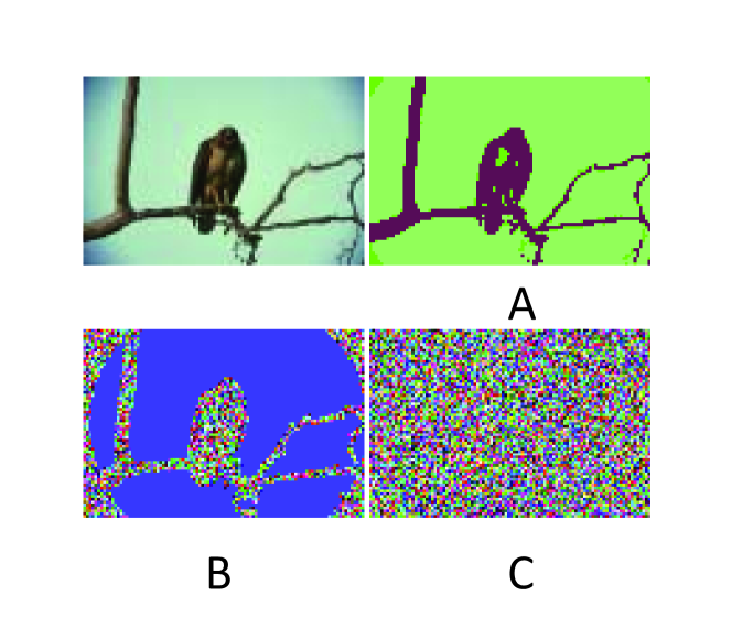
Figure 19: [Color Online.] The image segmentation results of the “bird” image. The original image is on the upper left. The segmentations denoted by “A”, “B” and “C” correspond to results with different parameter pairs ($\log(\gamma)$, $T$) that are marked in panel (a) of Fig. 18. Both results “A” and “B” are able to distinguish the “bird” from the “background”. However, in panel (b), the “bird” is composed of numerous of small clusters. The segmentation “C” does not detect the “bird”. The results shown here at points A, B, C correlate with the corresponding “easy-hard-unsolvable” phases in the phase diagram in Fig. 18.

Fig. 18 depicts the finite temperature ($T>0$) phase diagram of the image of the bird of Fig. 19. We will find that for this easy image, the phase boundaries between the easy, hard, and unsolvable phases of the image are relatively sharply defined.

In the context of the data to be presented, we fixed the background intensity $\bar{V}=15$, set the block size to be $L_{x}\times L_{y}=1\times 1$ and took the spatial scale $\ell\to\infty$. The varying parameters are the resolution $\gamma$ and temperature $T$. Instead of applying our community detection algorithm at zero temperature, we will incorporate the finite temperature dandan in this section. The ranges of the $\gamma$ and $T$ values are $[0.001,100]$ and $[0,1000]$ respectively. In the panels of Fig. 18, we show the normalized mutual information $I_{N}$, variation of information $V$, susceptibility $\chi$, energy $E$ and Shannon entropy $H$ as the function of the temperature $T$ and the logarithm of the resolution $\log(\gamma)$.

We can clearly distinguish the“easy”, “hard” and “unsolvable” phases from the 3D plots of $I_{N}$ (panel (a)), $V$ (panel (b)) and $H$ (panel (e)). The label“A” in panel (a) marks the “easy” phase, where $\gamma\in[0.001,0.3]$ for $T\in[0,500]$ and $\gamma\in[0.001,0.01]$ for $T\in[500,1000]$. The “easy” phase becomes narrower as temperature increases. The corresponding image segmentation result shown in Fig. 19 validates the label of the “easy” phase. The “A” image in Fig. 19 is obtained by running our community detection algorithm with the parameter pairs located in the area labeled by “A” in Fig. 18. The image segmentation denoted by “A” can perfectly detect the bird and the background. The bird is essentially composed of two clusters and the background forms one contiguous cluster. This reflects the true composition of the original image on the upper left. Thus, the bird image can be perfectly segmented in an unsupervised way when choosing parameters to be in the “A” region (corresponding to the computationally “easy” phase ).

The region surrounding point “B” in panel (b) in Fig. 18 denotes the “hard” phase, where $\gamma$ is in the range of $[0.3,100]$ and $T$ in the range of $[0,500]$. Within the “hard” phase, as the corresponding image labeled by “B” in Fig. 19 illustrates, the bird is composed of numerous small clusters with the background still forming one cluster. In this phase, the image segmentation becomes harder and some more complicated objects cannot be detected.

The label “C” in panel (c) in Fig. 18 denotes the “unsolvable” phase, where the range for $\gamma$ and $T$ is about $[0.1,100]$ and $[500,1000]$ respectively. The corresponding image in Fig. 19 labeled by “C” is composed of numerous small clusters for which it is virtually impossible to distinguish the bird from the background. In this phase, the normalized mutual information $I_{N}$ is far less than $1$ (indicating, as expected, the low quality of segmentations).

Other 3D plots in Fig. 18 generally show similar phase transitions. Especially, the 3D entropy plot (panel (e)) vividly depicts accurate three phases and their clear boundaries.

XII Conclusions

In summary, we applied a multi-scale replica inference based community detection algorithm to address unsupervised image segmentation. The resolution parameters can be adjusted to reveal the targets in different levels of details determined by extrema and transitions. In the images with uniform targets, we distributed edge weights based on the color difference. For images with non-uniform targets, we applied a Fourier transformation within blocks and assigned the edge weights based on an overlap. Our image segmentation results were shown to be, at least, as accurate as some of the best to date (see, e.g., Table. 1) for images with both uniform and non-uniform targets. The images analyzed in this work cover a wide range of categories: animals, trees, flowers, cars, brain MRI images, etc. Our algorithm is specially suited for the detection of camouflage images. We illustrated the existence of the analogs of three computational phases (“easy-hard-unsolvable”) found in the satisfiability ($k-$SAT) problem mezard1 ; mezard2 in the image segmentation problem as it was formulated in our work. When the system exhibits a hierarchal or general multi-scale structure, transitions further appear between different contending solutions. With the aid of the structure of the general phase diagram, optimal parameters for the image segmentation analysis may be discerned. This general approach of relating the thermodynamic phase diagram to parameters to be used in an image segmentation analysis is not limited to the particular Potts model formulation for unsupervised image segmentation that was introduced in this work. In an upcoming work, we will illustrate how supervised image segmentation with edge weights that are inferred from a Bayesian analysis with prior probabilities for various known patterns (or training sets), can be addressed along similar lines prep . We conclude with a speculation. It may well be that, in real biological neural networks, parameters are adjusted such that the system is solvable for a generic expected input and critically poised next to the boundaries between different contending solutions caudill .

Software.
The software package for the “multi-resolution community detection” algorithm peter1 that was used in this work is available at http://www.physics.wustl.edu/zohar/communitydetection/.

Acknowledgments
We wish to thank S. Chakrabarty, R. Darst, P. Johnson, B. Leonard, A. Middleton, D. Reichman, V. Tran, and L. Zdeborova for discussions and ongoing work and are especially grateful to Xiaobai Sun (Duke) for a very careful reading of the manuscript, comments, and encouragement.

Appendix A: Improved F-value by removing small high precision features

As seen in Sec. XI.3.1, our results in the first three images except the last one are better than the corresponding ones by the best algorithm in the Berkeley Image Segmentation Benchmark. One possible reason to cause the worse result in the last image is that our algorithm is too accurate. For example, the top image in Fig. 20, our result could detect the small white spray, which becomes the dots in the background. These small dots will form small circles in the boundary image shown in the right column, which are unexpected from the groundtruth, thus will reduce the value of precision and $F$. (In this case, $F=0.56$.)

Merging these high precision small dots with the background as, e.g., fleshed out in the second row in Fig. 20, leads to results that are equivalent to or better than those determined by the algorithm of global probability of boundary (gPb). A summary is presented in Table. 2.

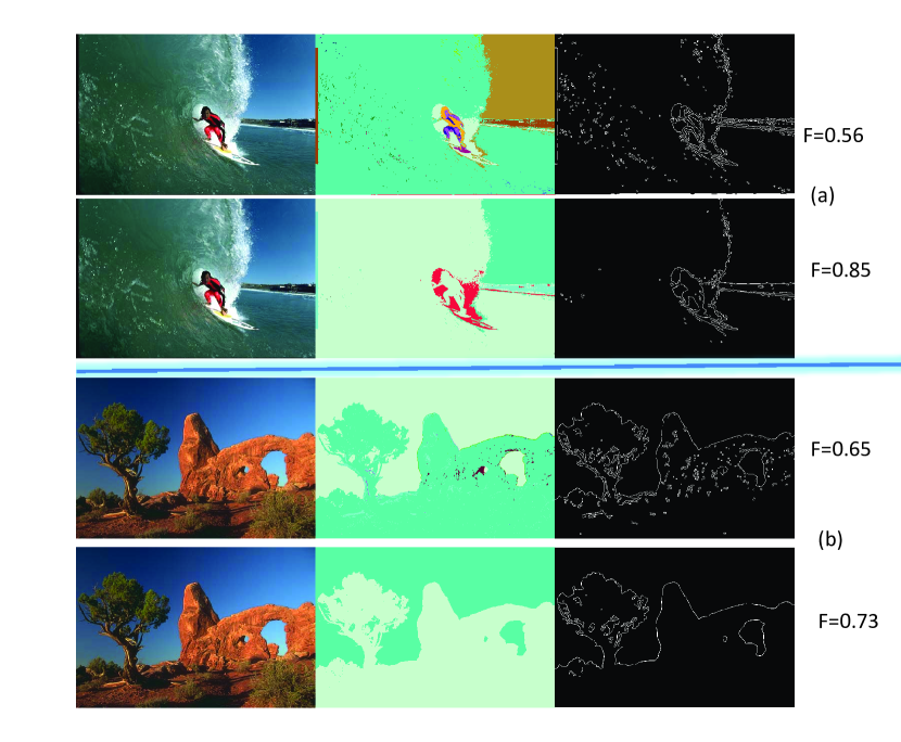
Figure 20: [Color Online.] The image segmentation results by our algorithm. The original images in the left most column are downloaded from Berkeley Image segmentation benchmark. The central image in the first row/ the third row is the result of our algorithm at $\gamma=0.01$ and $\bar{V}=20$. The right image in the first/the third row is the boundary detection result of the corresponding central image by the software Mathematica. There are many dots/circles which denote the white spray in original image in the first row. The small dots/circles in the third row denote the shadow in the original image. We merge these small dots in the first and third row into the background and the results shown in the second and fourth row are more smooth and close to the groundtruth. This is confirmed by the larger F value shown in Table. 2.

Appendix B: The image segmentation corresponding to the mutual information ($I_{N}$) peak

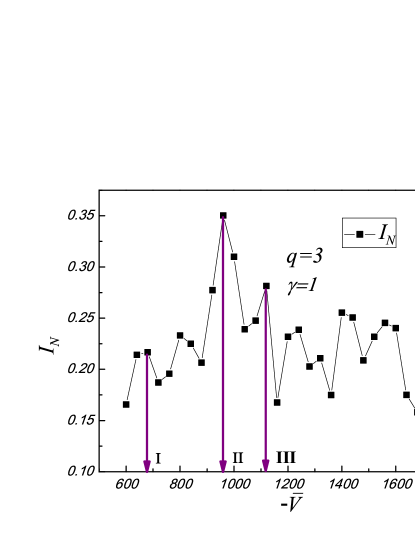
(a) The curve of $I_{N}$ as a function of negative threshold $-\bar{V}$ for the zebra image in panel (b).

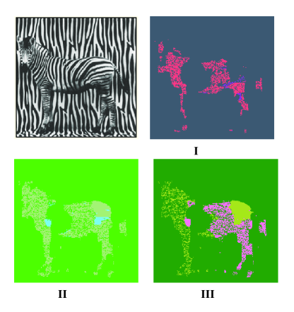
(b) The weighted result of the zebra images at the corresponding thresholds: $\bar{V}_{1}=-680$, $\bar{V}_{2}=-960$, and $\bar{V}_{3}=-1100$.

Figure 21: [Color Online] The “multiresolution” result of zebra with fixed community number $q=3$ and resolution $\gamma=1$. In panel(a), we plot the normalized mutual information $I_{N}$ as a function of negative threshold $\bar{V}$. The peaks in $I_{N}$ also correspond to the changes of structures. We choose three peaks and run the algorithm at these three particular thresholds, and the result images are shown in panel (b). As $|\bar{V}|$ increases, less regions in the zebra merge to the background, and the boundary becomes more clear.

As emphasized throughout this work, we focus on inter-replica information theory overlap extrema. In some of the earlier examples, we discussed the results pertaining to variation of information maxima (often correlating with normalized mutual information minima). We now briefly discuss sample results for the normalized mutual information maxima. We provide one such example in Fig. 21. Herein, we plot $I_{N}$ as a function of $\gamma$ and provide the corresponding segmented images at the peaks of $I_{N}$. As shown before, in panels I-III of Fig. 14, we provide the image segmentation that correspond to the values of $\gamma$ for which the variation of information $V$ exhibits a local maximum. In Fig. 21, we do the same for the normalized mutual information $I_{N}$.

Appendix C: The image segmentation with negative and positive Fourier weight

	F-Our algorithm	F-Our algorithm without noise	F-gPb
a	0.56	0.85	0.82
b	0.65	0.73	0.74

Table 2: The F-measure of the images shown in Fig. 20. We provide the comparison with the results by algorithm Global Probability of Boundary (gPb). Note that after removing the small dots/noise in both images, the value of F increase significantly. After this merger, our results become equivalent to (or even better than) the best results to date.

In this brief appendix, we wish to compare results obtained with the weights given by those of Eq. (11) to those obtained when $V_{ij}$ is set to be of the same magnitude as in Eq.(11) but of opposite sign (referred to below as its “negative counterpart”). In the latter case, a large weight $V_{ij}$ corresponds to a large overlap between patterns in blocks. Thus, minimizing the Hamiltonian will tend to fragment a nearly uniform background (for which the overlap between different blocks within is large) and will tend to group together regions that change. The results of the application of Eq. (11) and that of its negative counterpart are shown side by side in Fig. 22 II and III. In both cases, the zebra is successfully detected from the similar stripe-shaped background, as long as using the right parameters. In (II), the parameters used are as follows: the background $\bar{V}=-1200$, the resolution parameter is $\gamma=1$ and the block size is $l_{x}\times l_{y}=11\times 11$. In (III), we use a positive background $\bar{V}=900$ but with a negative Eq. (11), resolution $\gamma=1$ and block size $l_{x}\times l_{y}=7\times 7$. The difference shown in Fig. 22 between result (II) and (III) due to different fourier weights is that: In (II), the background forms a large cluster and the zebra is composed of lots of small clusters. In (III), the zebra forms a large single community while the background is composed of many small communities. For the images in Fig. 12, we substitute in Eq. (2), the weights of Eq. (11) along with a negative background $\bar{V}$.

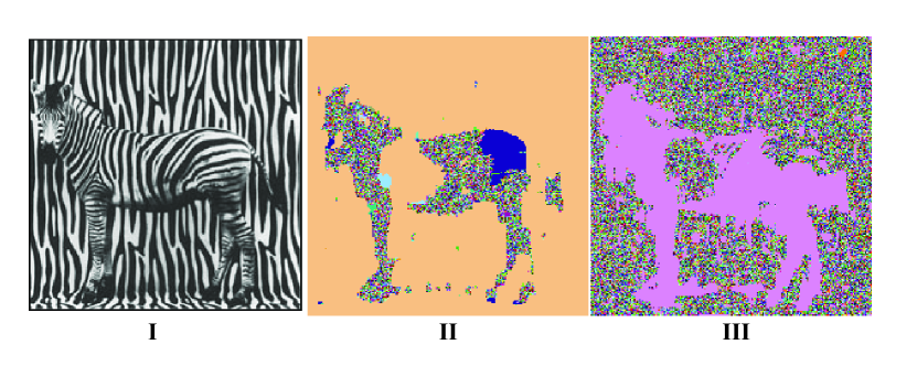
Figure 22: [Color Online.] The image segmentation results (II and III) of the original camouflaged zebra in (I). In panel (II), we used the Fourier based edge weights of Eq. (11) and with a negative background $\bar{V}=-1200$ (Other parameters are $\gamma=1$, block size $l_{x}\times l_{y}=11\times 11$). (III) The resulting segmentation when the sign on the right hand side of Eq. (11) is flipped. Here, we applied a positive background $\bar{V}=900$ (Other parameters are $\gamma=1$, block size $l_{x}\times l_{y}=7\times 7$). Both of the results shown here (i.e., II and III) are able to detect the zebra.

References

- (1) Y-J Zhang, Advances in Image and Video Segmentation, Editor IRM Press, (2006).
- (2) J. Bigun, Vision with Direction: A Systematic Introduction to Image Processing and Computer Vision, Springer, (2010).
- (3) L. O’Gorman, M. J. Sammon, and M. Seul, Practical Algorithms for Image Analysis, Cambridge University Press, (2008).
- (4) D. L. Pham, C. Xu, and J. L. Prince, Current Methods in Medical Image Segmentation, Annual Review of Biomedical Engineering, 2, 315-337 (2000).
- (5) R. Brunelli and T. Poggio, Face Recognition: Features versus Templates, IEEE transaction on pattern analysis and machine intelligence, 15, 10 (1993).
- (6) B. Bhanu, X. Tan, Computational algorithms for fingerprint recognition, Boston : Kluwer Academic Publishers (2004).
- (7) S. Carsten, M. Ulrich, and C. Wiedemann, Machine Vision Algorithms and Applications. Weinheim: Wiley-VCH. p. 1. ISBN 9783527407347 (2008).
- (8) M. Sezgin and B. Sankur, Survey over image thresholding techniques and quantitative performance evaluation, Journal of Electronic Imaging 13 (1): 146-165 (2003).
- (9) T. Kanungo, D. M. Mount, N. S. Netanyahu, C. D. Piatko, R. Silverman, A. Y. Wu, An efficient k-means clustering algorithm: Analysis and implementation. IEEE Trans. Pattern Analysis and Machine Intelligence 24: 881-892 (2002).
- (10) H. Mobahi, S. Rao, A. Yang, S. Sastry and Y. Ma, Segmentation of Natural Images by Texture and Boundary Compression, http://arxiv.org/abs/1006.3679 (2010).
- (11) O. Chapelle, P. Haffner, and V. N. Vapnik, Support Vector Machines for Histogram-Based Image Classification, IEEE Transactions on neural networks, 10, 5 (1999).
- (12) P. Meer, S. Wang, H. Wechsler, Edge detection by associative mapping, Pattern Recognition, 22, 491-504 (1989).
- (13) S. A. Hojjatoleslami and J. Kittler, Region Growing: A New Approach, IEEE Transaction on image processing, 7, No. 7, 1057-7149, p. 1079 (1998).
- (14) J. Kim, J. W. Fisher, A. Yezzi, M. Cetin, and A. S. Willsky, A Nonparameteric Statistical Method for Image Segmentation Using Information Theory and Curve Evolution, IEEE Transitions on Image Processing, 14, No. 10, 1057-7149, p. 1486 (2005).
- (15) C. Wojtan, N. Thürey, M. Gross, G. Turk, Deforming Meshes that Split and Merge. ACM Trans. Graph. 28, 3, Article 76 (2009).
- (16) S. Osher and N. Paragios, Geometric Level Set Methods in Imaging Vision and Graphics, Springer Verlag, ISBN 0387954880 (2003).
- (17) S. Fortunato, Community detection in graphs, Physics Reports 486, 75-174 (2010).
- (18) J. Shi, J. Malik, Normalized cuts and image segmentation, IEEE Transactions on Pattern Analysis and Machine Intelligence, 22, Issue 8, 888-905 (2000).
- (19) S. German and D. German, Stochastic Relaxation, Gibbs distributions and the Bayesian restoration of images, IEEE Transactions on Patterns, Anal. Mach. Intell. PAMI-6: 721 (1984).
- (20) J. L. Marroquin, Deterministic Bayesian Estimation of Markovian random fields with applications to computer vision, Proc. 1st Inter. Conf. Comput. Vision, London (1987).
- (21) E. B. Gamble and T. Poggio, Visual integration and detection of discontinuities: The key role of intensity edges, A. I. Memo No. 970, Artificial Intelligence Laboratory, MIT (1987).
- (22) D. Geiger and F. Girosi, Parallel and deterministic algorithms for MRFs: surface reconstruction and integration, PAMI-13(5) (1991).
- (23) S. Beucher, The Watershed Transformation Applied To Image Segmentation, Scanning Microscopy International, supp. 6, 299-314 (1992).
- (24) L. Grady, Random Walks from Image segmentation, IEEE Transaction on Pattern Analysis and Machine Intelligence, 28, No. 11 (2006).
- (25) L. Grady, E. L. Schwartz, Isoperimetric graph partitioning for image segmentation, IEEE Transactions on Pattern Analysis and Machine Intelligence, 28, Issue 3 (2006).
- (26) S.C. Amartur, D. Piraino and Y. Takefuji, Optimization neural networks for the segmentation of magnetic resonance images, IEEE Transactions on Medical Imaging, 11, No.2 (1992).
- (27) A. Kelemen, G. Szekely, G. Gerig, Three-dimensional model-based segmentation of brain MRI, Workshop on Biomedical image analysis, 4-13 (1998).
- (28) H. Trinh, Efficient Stereo Algorithm using Multiscale Belief Propagation on Segmented Images. In British Machine Vision Conference (BMVC) (2008).
- (29) B. Micusik and A. Hanbury, Steerable Semi-automatic Segmentation of Textured Images, Scandinavian Conference on Image Analysis (SCIA), Joensuu, Finland (2005).
- (30) M. Girvan and M. E. J. Newman, Community structure in social and biological networks, Proc. Natl. Acad. Sci. USA 99 (12): 7821 C7826 (2002).
- (31) S. Fortunato, Community detection in graphs, Phys. Rep. 486 (3-5): 75 C174 (2010).
- (32) M. E. J. Newman, Detecting community structure in networks, Eur. Phys. J. B 38 (2): 321 C330 (2004).
- (33) V. Gudkov, V. Montelaegre, S. Nussinov, and Z. Nussinov, Community detection in complex networks by dynamical simplex evolution, Phys. Rev. E 78, 016113 (2008)
- (34) http://www.eecs.berkeley.edu/Research /Projects/CS/vision/grouping/
- (35) http://www.psychologie.tu-dresden.de /i1/kaw/diverses%20Material /www.illusionworks.com/html/camouflage.html
- (36) P. Ronhovde, S. Chakrabarty, M. Sahu, K. K. Sahu, K. F. Kelton, N. Mauro, and Z. Nussinov, Detection of hidden structures on all scales in amorphous materials and complex physical systems: basic notions and applications to networks, lattice systems, and glasses, arXiv:1101.0008 (2011).
- (37) P. Ronhovde, S. Chakrabarty, D. Hu, M. Sahu, K. F. Kelton, N. A. Mauro, K . K. Sahu, and Z. Nussinov, Detecting hidden spatial and spatio-temporal structures in glasses and complex physical systems by multiresolution network clustering, arXiv:1102.1519 (2011).
- (38) P. Ronhovde and Z. Nussinov, Multiresolution community detection for megascale networks by information-based replica correlations. Phys. Rev. E 80, 016109 (2009).
- (39) R. B. Potts, Some Generalized Order-Disorder Transformations, Proc. Camb. Philos. Soc. 48, 106 C109 (1952).
- (40) S. Peng, B. Urbanc, L. Cruz, B. T. Hyman, and H. E. Stanley, Neuron recognition by parallel Potts segmentation, Proc. Natl. Acad. Sci. USA 100, 3847 C3852 (2003).
- (41) X. Descombes, M. Moctezuma, H. Maître, and J. P. Rudant, Coastline detection by a Markovian segmentation on SAR images, Signal Process. 55, 123-132 (1996).
- (42) K. Tanaka, Statistical-mechanical approach to image processing, J. Phys. A: Math. Gen. 35, R81 CR150 (2002).
- (43) F. W. Bentrem, A Q-Ising model application for linear-time image segmentation, Central European Journal of Physics, vol. 8, pp. 689-698 (2010).
- (44) P. Ronhovde and Z. Nussinov, Local resolution-limit-free Potts model for community detection. Phys. Rev. E 81, 046114 (2010).
- (45) S. Fortunato and M. Barthélemy, Resolution limit in community detection, Proc. Natl. Aca. Sci. U.S.A. 104, 36 (2007).
- (46) J. M. Kumpula, J. Saramäki, K. Kaski, andJ. Kertész, Limited resolution in complex network community detection with Potts model approach, Euro. Phys. J. B 56, 41 (2007).
- (47) M. Mézard, G. Parisi, R. Zecchina, Analytic and Algorithmic Solution of Random Satisfiability Problems, Science 297 812 (2002).
- (48) M. Mézard, A. Montanari, Information, Physics, and Computation, Oxford University Press, (2009).
- (49) Rather explicitly, there are four different cases to consider: (i) It is desirable to have nodes and in the same community if (i.e., if nodes and are linked). Thus, a negative energy is introduced for having nodes and in the same community (). (ii) It is undesirable to have nodes and in different communities if they linked ). Thus, a positive energy contribution is added in such a case. This is tantamount to augmenting the energy by . (iii) If nodes and are not linked () then an energy penalty should appear when putting them within the same community. This is captured by the term with . (iv) If nodes and are not linked then it is energetically favorable to have them in different communities. This leads to a negative contribution in the energy. Putting all of these pieces together and summing over all node pairs () leads, up to an innocuous additive constant, to the Hamiltonian of Eq. (1). All energy contributions are “absolute” and set by the existence of a link (or its absence) between the two members of each node pair without global (“null model” type) comparisons to other nodes in the system. An identical analysis in the case of more general weighted graphs leads to the Hamiltonian of Eq.(2) that will be employed in the current work for weighted images.
- (50) S. Mossa and G. Tarjus, Locally preferred structure in simple atomic liquids, J. Chem. Phys 119, 8069 (2003).
- (51) M. B. Hastings, Community Detection as an Inference Problem, Phys. Rev. E 74, 035102 (2006).
- (52) A. Decelle, F. Krzakala, C. Moore, L. Zdeborová, Phase transition in the detection of modules in sparse networks, arXiv:1102.1182 (2011).
- (53) D. Hu, P. Ronhovde, and Z. Nussinov, Phase transition in the community detection problem: spin-glass type and dynamic perspectives, arXiv:1008.2699 (2010).
- (54) C. Granell, S. Gómez, and A. Arenas, Mesoscopic analysis of networks: applications to exploratory analysis and data clustering, http://arxiv.org/abs/1101.1881v2 (2011).
- (55) P. Arbelaez, M. Maire, C. Fowlkes and J. Malik, Contour Detection and Hierarchical Image Segmentation, IEEE TPAMI, 33, No. 5, 898 (2011)
- (56) http://research.microsoft.com/en-us/projects/objectclassrecognition/
- (57) D. Martin, C. Fowlkes and J. Malik, Learning to Detect Natural Image Boundaries Using Local Brightness, Color, and Texture Cues, IEEE Transactions on Pattern Analysis and Machine Intelligence, VOL. 26, No.5, (2004).
- (58) M. Maire, P. Arbelaez, C. Fowlkes and J. Malik, Using Contours to Detect and Localize Junctions in Natural Images, Computer Vision and Pattern Recognition, (2008).
- (59) D. Shechtman, I. Blech, D. Gratias, J. Cahn, Metallic Phase with Long-Range Orientational Order and No Translational Symmetry, Phys. Rev. Lett. 53, 1951 (1984).
-
(60)
http://knowhowledge.com/website/staticpages/Edutainment
/Goldratio/Goldratiointro/goldratiointro2.asp - (61) A. van Blaaderen, Quasicrystals from nanocrystals, NATURE 461, 15 (2009).
- (62) http://en.wikipedia.org/wiki/Camouflage
- (63) D. Hu, P. Ronhovde, and Z. Nussinov, in preparation
- (64) M. S. Caudill, S. F. Brandt, Z. Nussinov, and R. Wessel, Parameter space analysis of delayed neural feedback triads, Phys. Rev. E 80, 051923 (2009)