Mean-field ’Temperature’ in Far From Equilibrium Systems

Abstract

We calculate the nonequilibrium mean-field ’temperature’ of a Brownian system in contact with a heat bath. We consider two different cases: an equilibrium bath in the presence of strong external forces and a nonequilibrium bath. By proving the existence of a generalized fluctuation-dissipation relation this mean-field ’temperature’ can be used to describe a nonequilibrium system as is if it were in thermal equilibrium with a thermal bath at the mean-field ’temperature’ mentioned above. We apply our results to chemical reactions in the presence of external forces showing how chemical equilibrium and Kramers rate constants are modified by the presence of these forces.
Keywords: Nonequilibrium ’temperature’, Fokker-Planck dynamics, Hamiltonian forces, Thermal forces, Effective reaction rates, Fluctuation theorem.

I Introduction

In the thermodynamic analysis of mesoscopic and macroscopic systems out of equilibrium an interesting question arises: Can we define a nonequilibrium ’temperature’? Although this is possible, this ’temperature’ cannot be a thermodynamic temperature since there is not a thermodynamic zero principle behind it. The consequences of this fact have been studied in detail in Ref.hernandez . Nevertheless, the concept of a nonequilibrium ’temperature’ can be used to parametrize the quasi-equilibrium states of a nonequilibrium system hernandez ,chetrite ,berthier ,granular ,berthier2 .

The notion of a nonequilibrium ’temperature’ can be made more precise by noting that this is a statistical concept related to the energy of a system involved in the erratic motion of its Brownian degrees of freedom, that is, related to the thermal energy of the system. Since the thermal energy of equilibrium and nonequilibrium systems will in general differ, one expects that the nonequilibrium ’temperature’ of an out of equilibrium system will be different from that of the heat bath. Introducing the nonequilibrium ’temperature’ has the advantage that one may describe the system as is if it were at thermal equilibrium with a hypothetical bath with a temperature corresponding to this nonequilibrium ’temperature’. This possibility has been studied for example for quantum corrections to the low temperature of thermodynamic systems or thermal radiation not in equilibrium in Ref. landau (page 104, section 34 and page 189, section 63, respectively) and in the case of granular matter in Ref. granular . Here, by using the nonequilibrium ’temperature’, we will show that in the case of chemical reactions an external force shifts chemical equilibrium and increases the reaction rates. This effect may be particularly important in the case of photochemistry where the incident light increases the velocity of the reaction.

In nonequilibrium systems such as small, confined or glass-like systems haxton , introducing a nonequilibrium ’temperature’ is appropriate since this concept is a consequence of the existence of internal constraints or long-range forces and correlations which maintain the system out of thermodynamic equilibrium. Some of these constraints may appear at low temperatures and for small masses as in the case of quantum effects landau mentioned above. In other cases, it is a purely classical effect when the range of the interactions is similar to the size of the system.

In this article, we propose a definition of the nonequilibrium ’temperature’ $T(a,t)$ in analogy with the equipartition theorem

$$k_{B}T(a,t)\rho(a,t)\equiv\int b^{2}f(b,a,t)db,$$ (1)

where $k_{B}$ is Boltzmann’s constant, $f(b,a,t)$ is a probability distribution describing the state of the system which, for convenience’s sake, we assume to depend on a pair of conjugated slow $a$ and fast $b$ variables (a velocity). In addition, $\rho(a,t)=\int f(b,a,t)db$ is a reduced probability distribution. One of the goals of this article consists of showing how this nonequilibrium ’temperature’, which we will call effective ’temperature’, is connected to the bath temperature and the forces which maintain the system out of equilibrium berthier . We also analyze how the fluctuation-dissipation theorem (FDT) is modified in systems far from equilibrium and how the effective ’temperature’ comes into play in order to extend the validity of this FDT to quasistationary nonequilibrium systems.

The paper is organized as follows: In section 2 we analyze Brownian motion in a field of force. We obtain the Fokker-Planck equation and a general expression for the effective ’temperature’ and its average value the mean-field ’temperature’. We also obtain the generalized Smoluchowski equation describing the quasi-equilibrium state. Section 3 is devoted to studying the effects of the mean-field ’temperature’ on chemical reaction rates. In section 4 we analyze the FDT. Finally, in section 5 we present our main conclusions.

II Brownian motion in a field of force

Let us consider a one dimensional Brownian gas in contact with a heat bath at temperature $T_{0}$ agusti . Let be $H(\Gamma)=mu^{2}/2+G(x)$ the Hamiltonian of a particle of mass $m$, where $\Gamma=(x,u)$ represents a point in the one-particle phase space and $G(x)$ being the external potential.

The analysis of this Brownian gas is based on thermodynamics through the definition of entropy by means of the Gibbs entropy postulate groot

$$S(t)=-k_{B}\int f\ln\frac{f}{f_{\textnormal{eq.}}}d\Gamma+S_{\textnormal{eq.}},$$ (2)

where $k_{B}$ is Boltzmann’s constant, $f(\Gamma,t)$ is the phase-space distribution function, $S_{\textnormal{eq.}}$ is the equilibrium entropy and

$$f_{\textnormal{eq.}}\sim\exp\left\{-\frac{H(\Gamma)}{k_{B}T_{0}}\right\},$$ (3)

is the equilibrium distribution function. Variations in the probability density $f(\Gamma,t)$ cause changes in the entropy which can be obtained from Eq. (2)

$$\delta S=-\int\left(k_{B}\ln\frac{f}{f_{\textnormal{eq.}}}+\frac{\mu_{\textnormal{eq.}}}{T_{0}}\right)\delta fd\Gamma,$$ (4)

where we have taken into account that $\delta S_{\textnormal{eq.}}=-\int$ $\left(\mu_{\textnormal{eq.}}/T_{0}\right)\delta fd\Gamma$. Here $\mu_{\textnormal{eq.}}(x,t)=-G(x)+\mu_{0}$ is the equilibrium chemical potential (mechanochemical potential) per unit of mass and $\mu_{0}(p,T_{0})$ is the corresponding thermodynamic potential, with $p$ being the pressure. By defining the nonequilibrium chemical potential

$$\mu(\Gamma,t)=k_{B}T_{0}\ln\frac{f}{f_{\textnormal{eq.}}}+\mu_{\textnormal{eq.}},$$ (5)

the thermodynamic quantity conjugated to the density $f(\Gamma,t)$, it is possible to write Eq.(4) in the compact way

$$T_{0}\delta S=-\int\mu(\Gamma,t)\delta f(\Gamma,t)d\Gamma$$ (6)

which constitutes the Gibbs equation in phase space.

A gradient of the chemical potential in phase space (5) induces a diffusion process which tends to restore the equilibrium state. Through this process, the distribution function changes according to the generalized Liouville equation

$$\frac{\partial}{\partial t}f(\Gamma,t)+v(\Gamma,t)\cdot\nabla_{\Gamma}f(\Gamma,t)=-\frac{\partial}{\partial u}J(\Gamma,t)$$ (7)

which defines the diffusion current $J(\Gamma,t)$ and where $v(\Gamma,t)=\left(\dot{x},\dot{u}\right)=\left(u,-\nabla G/m\right)$ is the velocity corresponding to the hamiltonian flow and $\nabla_{\Gamma}=\left(\nabla,\partial/\partial u\right)$, with $\nabla=\partial/\partial x$.

From Eq. (6) we can obtain the rate of change of the nonequilibrium entropy

$$\frac{dS}{dt}=-\frac{1}{T_{0}}\int\mu(\Gamma,t)\frac{\partial}{\partial t}f(\Gamma,t)d\Gamma$$ (8)

which in combination with Eq. (7) and after partial integration leads to

$$\frac{dS}{dt}=\frac{1}{T_{0}}\left\langle(-\nabla G)u\right\rangle-\frac{1}{T_{0}}\int J(\Gamma,t)\frac{\partial}{\partial u}\mu(\Gamma,t)d\Gamma.$$ (9)

Here, the first term on the right hand side of Eq. (9) is given by

$$\left\langle(-\nabla G)u\right\rangle=\int\left[-\nabla G(x)\right]uf(\Gamma,t)d\Gamma$$ (10)

and constitutes the power supplied by the external field which is dissipated in the system as heat. This contribution to the entropy change comes from the Hamiltonian evolution of the distribution function and therefore cannot be assimilated into the contribution due to diffusion. Thus, Eq. (10) can be interpreted as the rate of heat exchanged with the surroundings

$$\frac{dq}{dt}=\left\langle(-\nabla G)u\right\rangle,$$ (11)

with $dq$ being the amount of heat released in a time $dt$. In addition, the second term on the right-hand side of Eq. (9) constitutes the entropy production rate due to irreversible processes $\sigma$ which must be non-negative $(\sigma\geq 0)$ according to the second law. Therefore, the rate of change of entropy can be written in the compact way

$$\frac{dS}{dt}=\frac{1}{T_{0}}\frac{dq}{dt}+\sigma,$$ (12)

expressing the balance between the exchange of heat with the surroundings and the entropy generated in the irreversible processes established in the system. The entropy production contains the current $J(\Gamma,t)$ and its conjugated thermodynamic force $\left(\partial/\partial u\right)\mu(\Gamma,t)$. Following the postulates of nonequilibrium thermodynamics groot , these quantities are related through the phenomenological law

$$J(\Gamma,t)=-\frac{L}{T_{0}}\frac{\partial}{\partial u}\mu(\Gamma,t),$$ (13)

where $L$ is the phenomenological coefficient. By using the expression of the nonequilibrium chemical potential, Eq. (5) and Eq. (13) one obtains

$$J(\Gamma,t)=-\zeta\left(\frac{k_{B}T_{0}}{m}\frac{\partial}{\partial u}+u\right)f(\Gamma,t),$$ (14)

where we have identified $L/fT_{0}$ as the friction coefficient $\zeta$ of the Brownian particle ($L/fT_{0}\equiv\zeta/m$). Hence, from the definition of $\sigma$ given through Eq. (9), along with Eq. (14) we obtain

$$\sigma=\frac{m\zeta}{T_{0}}\int\frac{\left[(k_{B}T_{0}/m)\left(\partial/\partial u\right)f(\Gamma,t)+f(\Gamma,t)u\right]^{2}}{f(\Gamma,t)}d\Gamma.$$ (15)

It is worth to emphasize that a stationary nonequilibrium state ($dS/dt=0$) exist for which

$$\frac{1}{T_{0}}\frac{d_{st}q}{dt}=-\sigma_{st}.$$ (16)

This corresponds to a stationary state of nonzero entropy production which differs from the equilibrium state characterized by $d_{\textnormal{l.eq}}q/dt=\sigma_{\textnormal{l.eq}}=0$, a condition which is satisfied by the local Maxwellian (3).

Finally, by substituting Eq. (14) into Eq. (7) we obtain the Fokker-Planck equation describing the dynamics of the Brownian gas

$$\frac{\partial}{\partial t}f(\Gamma,t)=-u\nabla f+\nabla\left[\frac{G(x)}{m}\right]\frac{\partial}{\partial u}f+\zeta\left(\frac{k_{B}T_{0}}{m}\frac{\partial^{2}}{\partial u^{2}}f+\frac{\partial}{\partial u}uf\right).$$ (17)

III Effective and mean-field ’temperatures’

At this point, assuming that the velocity $u$ is the fast variable (in Brownian motion inertia usually constitutes a short lived effect), it is appropriate to write

$$f(\Gamma,t)=\phi_{x}(u,t)\rho(x,t),$$ (18)

where $\phi_{x}(u,t)$ is the conditional probability density and $\rho(x,t)=m\int f(\Gamma,t)du$ is the configurational probability density which evolves according to

$$\frac{\partial}{\partial t}\rho(x,t)=-\nabla\left[m\int uf(\Gamma,t)du\right].$$ (19)

Equation (18) expresses the coupling between the macroscopic process triggered by the field $G(x)$ and the microscopic process of the momentum relaxation ross . Equation (19) has been obtained by partial integration of Eq. (17) over velocity and thus implicitly defines the diffusion current $J(x,t)\equiv m\int uf(\Gamma,t)du\equiv\rho(x,t)v(x,t)$. This current satisfies the evolution equation

$$\frac{\partial}{\partial t}J(x,t)+\zeta J(x,t)=\rho(x,t)\left[-\nabla\frac{G(x)}{m}\right]-\nabla\left[\left(\int u^{2}\phi_{x}(u,t)du\right)\,\rho(x,t)\right],$$ (20)

obtained from Eq. (17) by multiplying by $u$ an integrating by parts with the appropriate boundary conditions. Here, the second moment of $\phi_{x}(u,t),\int u^{2}\phi_{x}(u,t)du$ is proportional to the thermal energy, i.e. the amount of energy of a system necessary for the erratic motion of its Brownian degrees of freedom. This suggests the definition of an effective ’temperature’

$$\frac{k_{B}T\left(x,t\right)}{m}=\overline{u^{2}}=\int u^{2}\phi_{x}(u,t)du$$ (21)

in analogy with the equipartition theorem berthier ,granular ,berthier2 . If in particular, the initial distribution is given by

$$f(\Gamma,0)=\rho(x,0)\exp\left\{-\frac{1}{2}\left(u-v(x,0)\right)^{2}m/k_{B}T_{0}\right\},$$ (22)

the solution of Eq. (17) at later times will have also the same Gaussian form and is given by (see Ref. groot CH. IX, $\S 8$)

$$f(\Gamma,t)=\rho(x,t)\exp\left\{-\frac{1}{2}\left(u-v(x,t)\right)^{2}m/k_{B}T_{0}\right\}.$$ (23)

In this case the second moment of $\phi_{x}(u,t)$ becomes

$$\overline{u^{2}}=\left[\frac{k_{B}T_{0}}{m}+v(x,t)^{2}\right]$$ (24)

which defines the effective ’temperature’

$$k_{B}T\left(x,t\right)=k_{B}T_{0}+mv(x,t)^{2}.$$ (25)

This effective ’temperature’ enters the expression of the diffusion current which, from Eq. (20) for long times as compared to $\zeta^{-1}$, reduces to

$$J(x,t)=-D(x,t)\left[\nabla\rho(x,t)+\frac{\rho(x,t)}{k_{B}T(x,t)}\nabla\Phi(x,t)\right],$$ (26)

where now $\Phi(x,t)=G(x)+k_{B}T(x,t)$ is an effective potential and $D(x,t)=(k_{B}T(x,t)/m)\zeta^{-1}$ is the bare effective diffusion coefficient. Substitution of Eq. (26) into (19) yields the generalized Smoluchowski equation

$$\frac{\partial}{\partial t}\rho(x,t)=\nabla\left\{D(x,t)\left[\nabla\rho(x,t)+\frac{\rho(x,t)}{k_{B}T(x,t)}\nabla\Phi(x,t)\right]\right\}.$$ (27)

If the conditions are such that the system is in a quasistationary state characterized by Eq. (16), thus, from Eqs. (11), (15) and ( 23) one obtains

$$v(x,t)=\zeta^{-1}\nabla\left[\frac{G(x)}{m}\right],$$ (28)

which implemented in Eq. (25) gives

$$k_{B}T\left(x,t\right)=k_{B}T_{0}+\frac{1}{m}\left[\zeta^{-1}\nabla G(x)\right]^{2}.$$ (29)

A particular simple case corresponds to the potential $G(x)=-Fx$ for which Eq. (29) reduces to

$$k_{B}T\left(t\right)=k_{B}T_{0}+\frac{1}{m}\left(\zeta^{-1}F\right)^{2}.$$ (30)

Another interesting particular case corresponds to the presence of thermal forces. The existence of, for example, an homogeneous temperature gradient in the bath brings the system to a nonequilibrium state. This non-homogeneous bath temperature $T_{\textnormal{nh}}(x)$ yields a Fokker-Planck equation in which $G(x)=\tilde{\gamma}\ln T_{\textnormal{nh}}$ with $\tilde{\gamma}$ a characteristic energy, mazur and therefore

$$k_{B}T\left(x,t\right)=k_{B}T_{\textnormal{nh}}+\frac{1}{m}\left(\gamma\zeta^{-1}\nabla\ln T_{\textnormal{nh}}\right)^{2}$$ (31)

Eqs. (29)-(31) show that when the system is subjected to a large force, the averaged kinetic energy related to Brownian motion increases, enabling one to define an effective ’temperature’ differing from the corresponding temperature of the bath.

In addition, for practical purposes it is convinient to introduce an estimate of the ’temperature’ field $T(x,t)$ which allows to incorporate the effects of the strong external forces in such a way that the usual techniques of nonquilibrium statistical physics can be used to calculate the properties of the system. In the lowest approximation, this can be done by means of the mean value $\langle T(x,t)\rangle=\int T(x,t)\rho(x,t)dx$, which we will call the mean-field ’temperature’ $T_{\textnormal{mf}}$:

$$k_{B}T_{\textnormal{mf}}(t)=k_{B}\left\langle T_{0}\right\rangle+\frac{1}{m}\langle\left[\zeta^{-1}\nabla G(x)\right]^{2}\rangle.$$ (32)

Adopting this mean-field ’temperature’, the current (26) takes the form

$$J(x,t)=-D\left[\nabla\rho(x,t)+\frac{\rho(x,t)}{k_{B}T_{\textnormal{mf}}}\nabla G(x)\right],$$ (33)

which, after substituted into Eq. (19), yields the generalized Smoluchowski equation

$$\frac{\partial}{\partial t}\rho(x,t)=D_{\textnormal{mf}}\nabla^{2}\rho(x,t)+\zeta^{-1}\nabla\left[\rho(x,t)\nabla G(x)\right],$$ (34)

where $D_{\textnormal{mf}}=(k_{B}T_{\textnormal{mf}}/m)\zeta^{-1}$ is the mean-field diffusion coefficient. At quasi-equilibrium, the solution of Eq. (34)

$$\rho_{\textnormal{qe}}(x)\sim\exp\left[-\frac{G(x)}{k_{B}T_{\textnormal{mf}}}\right],$$ (35)

is characterized by a mean-field thermal energy $k_{B}T_{\textnormal{mf}}$. In Eq. (35) we can interpret the mean-field ’temperature’ as the ’temperature’ for which the configuration probability density $\rho_{\textnormal{qe}}$ of the nonequilibrium system is equal to that given by Boltzmann’s probability distribution formula for a equilibrium system with ’temperature’ $T_{\textnormal{mf}}$. It is convenient to notice here that the previous results (33), (34) and (35) are exact when a constant force is applied on the system, because in this case Eqs. (30) and (32) are equivalent.

From the previous analysis, it is plausible to assume that inhomogeneities caused by the application of forces of different type may introduce similar effects in the dynamical properties of the system. For example, this will be the case of diffusion in the presence of a shear flow pre2001 ,pre2009 ,leporini . Finally, it is worth stress that introducing the mean-field ’temperature’ $T_{mf}$ is consistent only if $\Delta(mv^{2})<<k_{B}T_{0}$. Otherwise, the complete nonhomogeneous nonequilibrium effective ’temperature’ $T(x,t)$ has to be considered completely.

IV Modified chemical reaction rates

As an application of practical interest of the previous analysis, let us examine how the application of a large external force on a chemical system modifies the conditions of chemical equilibrium. In order to perform this analysis, we will assume that $x$ represents the reaction coordinate and that the reaction itself can be described as a diffusion process along the reaction coordinate agusti2 . For chemical systems $G(x)$ is the free energy controlling the reaction.

As in Ref. agusti2 , the current $J(x,t)$ given through Eq. (33) can be rewritten in the form

$$J(x,t)=-D_{\textnormal{mf}}\,e^{-G(x)/k_{B}T_{\textnormal{mf}}}\nabla e^{\mu_{\textnormal{mf}}(x,t)/k_{B}T_{\textnormal{mf}}},$$ (36)

where we have introduced the chemical potential

$$\mu_{\textnormal{mf}}(x,t)=k_{B}T_{\textnormal{mf}}\ln\rho+G(x).$$ (37)

When the height of the energy barrier separating the two minima of the potential is large compared to thermal energy, a fast relaxation towards the local minima occurs. Then, the chemical potential becomes a piece-wise continuous function of the coordinates

$$\mu_{\textnormal{mf}}(x,t)=\mu_{\textnormal{mf}}^{-}(x,t)\Theta(x_{0}-x)+\mu_{\textnormal{mf}}^{+}(x,t)\Theta(x-x_{0}),$$ (38)

with $\mu_{\textnormal{mf}}^{-}$ and $\mu_{\textnormal{mf}}^{+}$ referring to the chemical potential at the left and right wells, respectively. Consequently the probability density also splits as

$$\rho(x,t)=\rho_{1}(t)e^{-\left[G(x)-G(x_{1})\right]/k_{B}T_{\textnormal{mf}}}\Theta(x_{0}-x)+\rho_{2}(t)e^{-\left[G(x)-G(x_{2})\right]/k_{B}T_{\textnormal{mf}}}\Theta(x-x_{0}),$$ (39)

here $\rho_{i}(t)=\rho(x_{i},t)$ with $i=1,2$ are the values of the probability density at the minima, $\Theta(x)$ is the step function and $x_{j}$ with $j=0,1,2$ are the coordinates of the maximum and the minima of the potential, respectively.

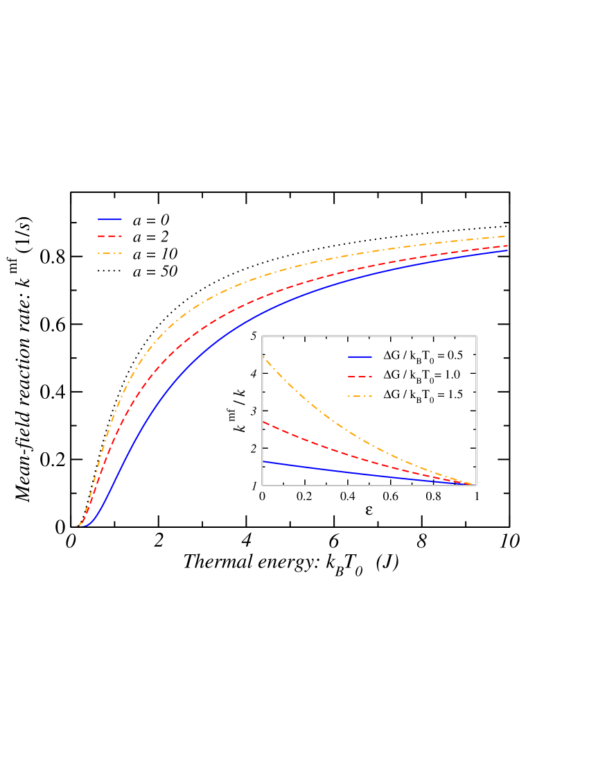
Figure 1: Schematic representation of the mean-field reaction rate $k_{\textnormal{mf}}$ as a function of the temperature of the bath for different values of the correction term $a=\frac{1}{m}\langle(\zeta^{-1}\nabla G)^{2}\rangle$ with $\Delta G=1$ and $D_{\textnormal{mf}}\sqrt{G^{\prime\prime}(x_{2,1})|G^{\prime\prime}(x_{0})|}/({2\pi k_{B}T_{\textnormal{mf}}})=1$. The inset shows the ratio $k^{\textnormal{mf}}/k$ of reaction rates as a function of $\epsilon=T_{0}/T_{\textnormal{mf}}$ for three different values of $\Delta G/k_{B}T_{0}$. When the force associated to the energy $G(x)$ is large the thermal energy is large enough to increase the mean-field reaction rate.

Starting from the mean-field Smoluchowski equation (34) and using relations (36)-(39), it is possible to derive the following kinetic equation for the concentrations $\rho_{i}$

$$\frac{d\rho_{1}}{dt}=-\frac{d\rho_{2}}{dt}=k_{+}^{\textnormal{mf}}\rho_{2}-k_{-}^{\textnormal{mf}}\rho_{1},$$ (40)

where the forward and backward reaction rates are given by

$$k_{+,-}^{\textnormal{mf}}=D_{\textnormal{mf}}\frac{\sqrt{G^{\prime\prime}(x_{2,1})|G^{\prime\prime}(x_{0})|}}{2\pi k_{B}T_{\textnormal{mf}}}exp\left[\frac{G(x_{2,1})-G(x_{0})}{k_{B}T_{\textnormal{mf}}}\right].$$ (41)

From this equation it follows an interesting result that can be expressed as the ratio between the mean-field rate $k^{\textnormal{mf}}$ and the reaction rate when no external field is applied $k$: $k^{\textnormal{mf}}/k=exp\left(\Delta G/k_{B}T_{0}\right)exp[-\left(\Delta G/k_{B}T_{0}\right)\epsilon]$ where $\epsilon=T_{0}/T_{\textnormal{mf}}$ is a measure of the deviation from thermal equilibrium and $\Delta G=G(x_{0})-G(x_{2,1})$ that is a positive quantity by definition jpcm2004 ,kegel . Figure 1 shows $k^{\textnormal{mf}}/k$ as a function of $\epsilon$. It is clear that the external force shifts the chemical equilibrium and increases the reaction rates. This is particularly interesting in photochemical reactions because the correction involved in the mean-field ’temperature’ is proportional to the energy of the electromagnetic field, that is to the number of photons associated to the incident light. Another interesting case is when the chemical reactions take place in a nonequilibrium medium like alive organisms or chemical reactors in which the presence of thermal or concentration gradients as well as hydrodynamic flows modify the chemical equilibrium.

V Generalized fluctuation-dissipation theorem

Once the generalized Smoluchowski equation (34) has been formulated, it is convenient to derive the generalized fluctuation-dissipation theorem which relates the time derivative of the correlation function $C_{AF}(t,t^{\prime})$ with the response function $R_{AF}(t,t^{\prime})$ of an observable $A(x)$ through the mean-field ’temperature’ when at time $t=t_{0}$ the system is perturbed by the external field $F(x,t)$ berthier2 ,kubo ,ocio . As a consequence of this and in analogy with slow relaxing systems chetrite , the generalized fluctuation-dissipation theorem offers a statistical tool in order to evaluate the mean-field ’temperature’.

For a sufficiently weak perturbation around the quasi-equilibrium state characterized by Eq. (35) and the mean-field ’temperature’ $T_{\textnormal{mf}}$, the response of the system can be expressed in terms of the deviation of the average value $\langle A(t)\rangle_{F}$ in the presence of the force field $F$ with respect to the unperturbed case $\langle A(t)\rangle_{\textnormal{qe}}$:

$$\langle A(t)\rangle_{F}-\langle A(t)\rangle_{\textnormal{qe}}=\int_{t_{0}}^{t}R_{AF}(t,t^{\prime})F(t^{\prime})dt^{\prime},$$ (42)

where we have defined

$$\langle A(t)\rangle_{F}=\int A(x)\rho_{F}(x,t)dx\,\,\,\,\,\,\text{and}\,\,\,\,\,\,\langle A(t)\rangle_{\textnormal{qe}}=\int A(x)\rho_{\textnormal{qe}}(x,t)dx.$$ (43)

To obtain an explicit expression for the left-hand side of Eq. (43), we may use the fact that the perturbed probability density $\rho_{F}$ satisfies the identity

$$\rho_{F}(x,t)=\int G_{F}(x,t|x^{\prime},t^{\prime})\rho_{F}(x^{\prime},t^{\prime})dx^{\prime},$$ (44)

where $G_{F}(x,t|x^{\prime},t^{\prime})$ is the Green function in the presence of the perturbation. Considering also that the quasi-equilibrium solution of Eq. (34) in the presence of the perturbation $F$ is: $\rho_{\textnormal{qe}}^{F}=\rho_{\textnormal{qe}}Z_{F}(x,t)$, with $Z_{F}(x,t)\equiv Z[F(x,t)]$ a functional of the perturbation field $F$. Now, after substituting $\rho_{\textnormal{qe}}^{F}$ in Eq. (44) and rearranging terms one obtains

$$\rho_{\textnormal{qe}}(x,t)=\int G_{F}(x,t|x^{\prime},t^{\prime})\frac{Z_{F}(x^{\prime},t^{\prime})}{Z_{F}(x,t)}\rho_{\textnormal{qe}}(x^{\prime},t^{\prime})dx^{\prime}.$$ (45)

Using Eq. (45) and the fact that $\rho(x,t)=\int G(x,t|x^{\prime},t^{\prime})\rho(x^{\prime},t^{\prime})dx^{\prime}$ with $G(x,t|x^{\prime},t^{\prime})$ the unperturbed Green function, we may establish the quasi-equilibrium fluctuation relation

$$G_{F}(x,t|x^{\prime},t^{\prime})=\frac{Z_{F}(x,t)}{Z_{F}(x^{\prime},t^{\prime})}G(x,t|x^{\prime},t^{\prime}),$$ (46)

which expresses the perturbed Green function in terms of the unperturbed one. Now, using that $\rho_{F}(x,t_{0})=\rho_{\textnormal{qe}}(x,t_{0})$ at $t^{\prime}=t_{0}$, then the following relation holds

$$\rho_{F}(x,t)=\int G_{F}(x,t|x^{\prime},t_{0})\rho_{\textnormal{qe}}(x^{\prime},t_{0})dx^{\prime}.$$ (47)

The substitution of Eq. (47) in Eq. (43) leads, after using the fluctuation relation (46), to the formula

$$\langle A(t)\rangle_{F}=\int\int A(x)\frac{Z_{F}(x,t)}{Z_{F}(x^{\prime},t_{0})}G(x,t|x^{\prime},t_{0})\rho_{\textnormal{qe}}(x^{\prime},t_{0})\,dxdx^{\prime}.$$ (48)

Here, Eq. (48) may be written in a form similar to Eq. (42) by approximating ${Z[F(x,t)]}/{Z[F(x^{\prime},t_{0})]}$ in its series expansion up to first order in $F$. This operation gives the integral relation

$$\langle A(t)\rangle_{F}-\langle A(t)\rangle_{\textnormal{qe}}=\int\int A(x)\left[F(x,t)-F(x^{\prime},t_{0})\right]G(x,t|x^{\prime},t_{0})\rho_{\textnormal{qe}}(x^{\prime},t_{0})\,dxdx^{\prime}.$$ (49)

Recalling now that for the Smoluchowski operator

$$Z[F(x,t)]=\frac{exp(F_{0}B(x)/k_{B}T_{\textnormal{mf}})}{\langle exp(F_{0}B(x)/k_{B}T_{\textnormal{mf}})\rangle},$$ (50)

where we have used $F(x,t)=F_{0}dB(x)/dx$ for convenience and assumed that $F_{0}$ is a constant agusti . Therefore, using (50) in Eq. (49), for weak perturbations $exp(F_{0}B/k_{B}T)\sim 1-F_{0}B/k_{B}T$ and we obtain

$$\langle A(t)\rangle_{F}-\langle A(t)\rangle_{\textnormal{qe}}=F_{0}\left[\frac{1}{k_{B}T_{\textnormal{mf}}(t)}C_{AB}(t,t)-\frac{1}{k_{B}T_{\textnormal{mf}}(t_{0})}C_{AB}(t,t_{0})\right],$$ (51)

where $C_{AB}(t,t_{0})=\langle A(t)B(t_{0})\rangle-\langle A(t)\rangle\langle B(t_{0})\rangle$. Assuming now that the quasi-stationary state of the system varies slowly enough, then we can replace $T_{\textnormal{mf}}(t)$ by $T_{\textnormal{mf}}(t_{0})$ in (51). The resulting expression can then be written as the integral of the time derivative of the correlation function which, after being compared with Eq. (42) finally gives

$$R_{AB}(t,t_{0})=\frac{1}{k_{B}T_{\textnormal{mf}}(t_{0})}\frac{\partial}{\partial t_{0}}C_{AB}(t,t_{0})$$ (52)

which constitutes the quasi-equilibrium fluctuation-dissipation relation valid for times $t>t_{0}$. This result implies that the fluctuation-dissipation relation can be generalized to the quasi-equilibrium state by incorporating the corrections on system’s temperature due to the large potential $V(x)$, agusti ,jcp2004 . Clearly, this result is fully compatible with the quasi-equilibrium fluctuation relation (46).

VI Conclusions

In this paper we have introduced the concepts of nonequilibrium effective ’temperature’ $T(x,t)$ and its average value, the mean-field ’temperature’ $T_{\textnormal{mf}}$, by using a generalization of the equipartition theorem. This mean-field ’temperature’ parametrizes the quasi-equilibrium or metastable states of a nonequilibrium system. This parameter reveals that in the presence of large external forces the thermal energy of the system increases, therefore promoting the thermal motion of its corresponding degrees of freedom.

We have shown that at equilibrium this mean-field ’temperature’ reduces to the bath temperature while at quasi-equilibrium it contains quadratic corrections coming from the forces, either Hamiltonian or thermal, acting on the system. The existence of internal constraints like surface effects or long-range forces would lead to similar phenomena as the ones arising from the applied external forces.

Once this mean-field ’temperature’ has been introduced, we can describe a nonequilibrium system as is if it were in equilibrium with a thermal bath at this $T_{\textnormal{mf}}$ since it has been proven that fluctuations in a nonequilibrium system satisfy a generalized fluctuation-dissipation theorem containing $T_{\textnormal{mf}}$.

We have illustrated the possible implications in practical situations by analyzing how external forces modify the chemical equilibrium and the Kramers reaction rates. We point out that external forces increase the reaction rates, such as in photochemical reactions or in the presence of nonequilibrium substrates.

Figure 2:

References

- (1) Popov, A. V.; Hernandez, R. J. Chem. Phys. 2007, 126, 244506.
- (2) Chetrite, R. Phys. Rev. E 2009, 80, 051107.
- (3) Berthier, L; Barrat, J.-L. J. Chem. Phys. 2002, 116, 6228.
- (4) Ippolito, I.; Annic, Ch.; Lemaître, J.; Oger, L. and Bideau, D. Phys. Rev. E 1995, 52, 2072.
- (5) Berthier, L. and Barrat, J.-L. Phys. Rev. Lett. 2002, 89, 095702.
- (6) Landau, L. D.; Lifshitz, E. M. Statistical Physics, Part 1; Pergamon Press, 1980.
- (7) Haxton, T.K. and Liu, A. J. Phys. Rev. Lett. 2007, 99, 195701.
- (8) Pérez-Madrid, A.; J. Chem. Phys. 2005, 122, 214914.
- (9) de Groot, S.R.; Mazur, P. Non-Equilibrium Thermodynamics; Dover, New York, 1984.
- (10) Ross, J.; Mazur, P. J. Chem. Phys. 1961, 35, 19.
- (11) Pérez-Madrid, A.; Rubí, J.M.; Mazur, P. Physica A 1994, 212, 231.
- (12) Santamaría-Holek, I.; Reguera, D.; Rubi, J. M. Phys. Rev. E 2001, 63, 051106.
- (13) Santamaría-Holek, I.; Barrios, G.; Rubi, J. M. Phys. Rev. E 2009, 79, 031201.
- (14) Mauri, R.; Leporini, D. Europhys. Lett. 2006, 76, 10221028.
- (15) Pagonabarraga, I.; Pérez-Madrid, A. and Rubí, J.M. Physica A 1997, 237, 205.
- (16) Rubi, J.M.; Santamaría-Holek, I.; Pérez-Madrid, A. J. Phys.: Condens. Matter 2004, 16, S2047 .
- (17) Bonn D.; Kegel W. K. J. Chem. Phys. 2003, 118, 2005.
- (18) Kubo, R.; Toda, M.; Hashitsume, N. Statistical Physics, Part II; Springer, Berlin, 1991.
- (19) Hérisson, D.; Ocio M. Phys. Rev. Lett. 2002, 88, 257202.
- (20) Santamaría-Holek, I.; Pérez-Madrid, A; Rubi, J. M. J. Chem. Phys. 2004, 120, 2818.