Stability Peninsulas on the Neutron Drip Line

Abstract

Using HF+BCS method with Skyrme forces we analyze the neutron drip line. It is shown that around magic and new magic numbers the drip line may form stability peninsulas. It is shown the location of these peninsulas does not depend on the choice of Skyrme forces. It is found that the size of the peninsulas is sensitive to the choice of Skyrme forces and the most extended peninsulas appear with the SkI2 set.

One of the major problems in nuclear physics having also interdisciplinary importance is the positioning of the neutron drip line. The microscopic approaches to the study of neutron rich nuclei include the Hartree-Fock-Bogoliubov (HFB) and Hartree-Fock (HF) methods using effective forces, see f. e. 2 ; 4 ; 5 or relativistic meanfield (RMF) theory 6 . The standard theoretical procedure in locating the neutron drip line is to take a stable nucleus and load it with neutrons until it saturates, that is adding extra neutrons makes the isotope undergo the neutron decay thereby releasing these extra neutrons. This method, however, implies a simple structure of the drip line, namely, that any straight line on the nuclear chart, which corresponds to a fixed number of protons, crosses the neutron drip line only once. Yet it might happen that the drip line has a more complicated structure. In the vicinity of magic numbers or new magic numbers the following scenario can take place. At some point $(N,Z)$ nuclei loose their stability but then after gaining more neutrons their stability becomes restored. This leads to the formation of stability peninsulas on the nuclear chart.

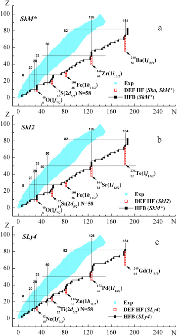
Figure 1: (Color online). The nuclear chart and the 1n drip line. Filled blue area shows experimentally known nulei. The solid line going through the dark squares is the 1n drip line in HFB calculations 4 . Red empty squares a nuclei stable against 1 neutron emission according to DEF HF calculations with SkM* (a), SkI2 (b) and SLy4 (c) forces. The dotted line goes corresponds to magic numbers $N=8,20,28,50,82,126,184$ and to the new magic number N=32.

This scenario of formation of stability peninsulas has been analyzed by us in Refs.  9 ; 11 ; 12 ; 13 ; 14 ; 15 ; 16 ; 16.1 for the isotopes of O, Ar, Ni, Zr, Kr, Pb, Rn and other elements. The calculations were performed using the HF+BCS approach with Skyrme forces accounting for deformations (DEF HF approach). In 12 ; 13 ; 14 ; 15 ; 16 we have analyzed the mechanism, which leads to the stability restoration. It turns out that nuclei lying close to such peninsulas possess low–lying quasistable one–particle states. By adding neutrons one makes these levels dive into the discrete spectrum, thus stabilizing the isotope. The stability restoration by additional neutrons was also observed in 16.2 , where the authors use the D1S Gogny force.

The discussion of the DEF HF method one finds in 11 ; 17 ; 18 ; 19 . The DEF HF calculations are performed using the deformed harmonic oscillator basis, where the basis parameters are optimized on each iteration, for details see 11 . The optimization procedure consists in choosing optimal oscillator frequencies, which minimize the total energy within a given basis. Let us mention that the optimization procedure facilitates the calculation and, more important, corrects the basis functions for the spatially extended density distributions near the drip line 11 . The pairing constant is set to $G=(19.5/A)[1\pm 0.51(N-Z)/A]$, where the plus and minus signs refer to protons and neutrons respectively. In DEF HF calculations we include only bound one particle states. In spite of ignoring the continuum states this method still provides a good agreement with the HFB, see 12 ; 13 ; 14 ; 15 ; 16 . Since all nuclei, which lie on the stability peninsulas are spherical we also use a spherical code (SPH HF) 19.1 , which solves the HF equations directly rather than using a particular basis. In the BCS scheme of the spherical code we implement the inclusion of localized quasibound continuum states, which are confined under the centrifugal barrier. The size of the box used to discretize the continuum is set to 50 fm. The quasi bound state is considered localized if the probability to find the particle beyond the radius corresponding to the maximum of centrifugal barrier is less than 50%.

We used the following sets of Skyrme forces Ska, SkM*, SLy4, and SkI2, see 20 ; 21 ; 22 ; 23 and references therein (below under Skyrme forces we shall mean only these sets of forces). Stability peninsulas originate for all Skyrme forces, which produce low–lying quasibound one–particle states with high angular momentum (which are responsible for a high centrifugal barrier confining the particles).

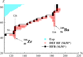
Figure 2: (Color online). A detailed fragment of Fig. 1. The notations are that of Fig. 1.

By definition the one or two neutron separation energies on these lines would be very small, sometimes within 0.1 Mev. Unfortunately, various Skyrme forces do not agree with each other over the whole nuclear chart to that degree of accuracy. So it would be naive to expect that different Skyrme forces would all predict a unique neutron drip line. However, all Skyrme forces predict the same magic and new magic numbers. The observed stability peninsulas with respect to one neutron emission are shown in Fig. 1 for different Skyrme forces. It is easy to see from Fig. 1 that the formation of peninsulas on the neutron drip line happens at the same N values for all forces but peninsula edges have different Z values.

It should be stressed that nuclei forming stability peninsulas are spectrally bound in the sense that there exists a well-defined ground state wave function, which minimizes the energy functional for such nuclei. At this point they become well-defined compact objects and the question about their lifetime becomes correctly formulated. And though for some nuclei it may be energetically favorable to get rid of two or more neutrons, a large centrifugal barrier of the last filled levels may serve as an indication that this lifetime would be large. Let us also mention that all spectrally stable nuclei in our calculations appear as such in grid calculations based on the code from 23.05 .

We found that Ska and SkM* forces occupy an intermediate position between SkI2 and SLy4, in the sense that more elements are stable with SkI2 and less with SLy4. The forces SkI2 are the most optimistic, at the same time the formation of stability peninsulas for SLy4 is rather rare. The difference between two of these forces is depicted in Fig. 1.

In Fig. 1 one finds the comparison with benchmark HFB calculations 4 . The position of 1n drip line in 4 is obtained from the condition $\lambda_{n}=0$. In our method we use the Koopmans theorem to approximate one neutron separation energies $S_{n}$ and define the drip line by condition $S_{n}=0$, where even small positive $S_{n}$ indicates the stability against the one–neutron emission. Note that within HF and HFB methods one neutron separation energies can be calculated only using certain approximations 16.2 ; 31 and 1n drip lines determined from the conditions $\lambda_{n}=0$ and $S_{n}=0$ may not necessarily coincide 16.2 .

1n drip line in Fig. 1 for various Skyrme forces has typical bend points around known magic numbers $N=82$ (SLy4), $N=126$ (SkM*, SkI2, SLy4), $N=184$ (SkM*, SkI2, SLy4) and also for $N=32$ (SkM*, SkI2) and $N=58$ (SkM*, SkI2, SLy4). The bend points indicate the stability enhancement around these $N$–values. It is worth noting that the stability peninsulas are formed for various Skyrme forces around the same neutron numbers. As we have already mentioned the stability restoration results from low–lying quasibound states, which immerse into the bound spectrum for higher $N$ 12 ; 13 ; 14 ; 15 ; 16 .

Below we list the stable isotopes that form stability peninsulas and the responsible subshells for the Skyrme forces SkM* and Ska. $1f_{7/2}$ – ⁴⁰O; $2d_{5/2}$ – ⁷⁶Ar, ⁷⁴S; $1h_{11/2}$ – ¹¹⁰Ni, ¹⁰⁸Fe; $1i_{13/2}$ – ¹⁷⁴Cd, ¹⁷²Pd, ¹⁷⁰Ru, ¹⁶⁸Mo, ¹⁶⁶Zr; $1j_{15/2}$ – ²⁵⁶Hf, ²⁵⁴Yb, ²⁵²Er, ²⁵⁰Dy, ²⁴⁸Gd, ²⁴⁶Sm, ²⁴⁴Nd, ²⁴²Ce, ²⁴⁰Ba. From Fig. 1 it can be seen that the stability peninsulas with SkI2 forces are by one or two $Z$ longer than those formed with SkM*. For $N=184$ the last stable isotope with SkI2 forces is ²³⁶Te having $Z=52$, which is close to the magic $Z=50$. The neutron to proton ratio in ²³⁶Te reaches $N/Z=3.54$. In the case of ⁴⁰O one has $N/Z=4$! For SLy4 forces the whole nuetron drip line becomes shifted in the positive $Z$ direction and the edges of stability peninsulas are formed by the isotopes ⁴²Ne; ⁸⁰Ti, ¹¹²Zn, ¹⁷²Pd, ²⁴⁸Gd.

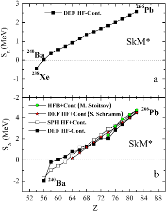
Figure 3: (Color online). One and two neutron separation energies for the series of isotones corresponding to $N=184$ for SkM* forces. (a) One neutron separation energies in DEF HF calculations without continuum states in the BCS scheme. (b) two–neutron separation energies. Dark squares are DEF HF calculations (without continuum in the BCS). Light squares are SPH HF calculations with continuum states. Red stars are DEF HF in grid calculations with continuum states. Green circles are HFB calculations 4 .

For all Skyrme forces the nuclei forming stability peninsulas are spherical in DEF HF calculations, which is characteristic of magic numbers. The spherical form allows to run additional check with SPH HF method, where pairing is treated more precisely. Such additional calculations were done for ⁴⁰O, ⁷⁴S, ¹⁰⁸Fe, ¹⁶⁶Zr and ²⁴⁰Ba using SkM*, and taking into account localized states with $n\leq 10$ and $l\leq 14$. The pairing contribution for these nuclei was equal to zero, which testifies for the magicity of corresponding neutron numbers. Let us add that ⁷⁴S (SkM*, Ska), ⁷²Si (SkI2) and ⁸⁰Ti (SLy4) have $N=58$, which is close to $N=56$, whose magicity is discussed in 32 . The treatment of quasi–bound states in the pairing scheme is done similar to 33 ; 34 .

The most impressively extended stability peninsula occurs at $N=184$. Fig. 2 shows the fragment of the neutron drip line around $N=126$ and $N=184$. One can see that that the peninsulas broaden with higher $Z$. The shift of the drip line compared to HFB calculations results from the different conditions for its determination, namely, zero one neutron separation energy (in the Koopman’s approximation) in our case and zero chemical potential in the HFB method.

Fig. 3 shows one neutron separation energies for the isotone chain $N=184$ (SkM* forces). One can see that $S_{n}$ and $S_{2n}$ decrease monotonically. The nucleus ²⁴⁰Ba lies on the edge of stability peninsula, its one neutron separation energy is very small $S_{n}=0.024$ Mev (DEF HF calculation) and $S_{n}=0.064$ MeV (SPH HF calculation). The last filled one–particle level is 1$j_{15/2}$, which produces the HF potential with the centrifugal barrier height of 8.58 MeV.

Two neutron separation energies for isotones corresponding to $N=184$ are shown in Fig. 3. For $Z=56,58,60$ we used the binding energies of the isotopes are not stable against one neutron emission. This might, of course, reduce the precision of $S_{2n}$ values. One can see that DEF HF, SPH HF and HFB calculations are in good agreement. The nucleus ²⁴⁸Gd, which has $Z=64$ has a positive $S_{2n}$ value. Thus for $N=184$ the stability peninsula contains isotopes that are stable against both one and two–neutron emission. We compared our method to a computer program using a different numerical approach based on solving the equations on a two-dimensional spatial grid 23.05 , using a delta force for the BCS pairing interactions. A typical comparison of the methods can be seen in Fig. 3.

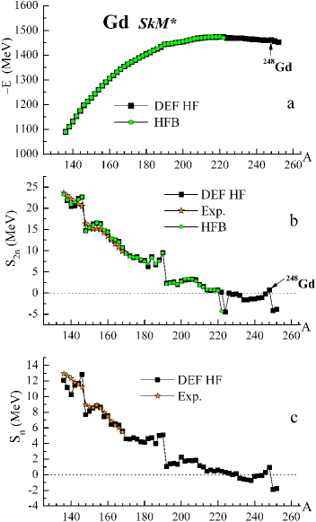
Figure 4: (Color online). Total binding energy (a) and two-neutron (b) and one –neutron (c) separation energies for neutron rich Gd isotopes. Orange stars show the experimental data 37 . Dark squares are DEF HF calculations with SkM* forces. Green circles represent the HFB data 4 .

In the early papers 35 ; 36 we showed that DEF HF with Skyrme forces provides a satisfactory description in the region of rare earth elements over a wide mass range. Let us take a closer look at the chain of Gd isotopes. Fig. 4 shows that separation and binding energies are in good agreement with existing HFB calculations 4 . On the figures these values are at some places practically indistinguishable. The plots excellently fit the existing experimental data 37 as well.

In the DEF HF approach the first loss of stability against 2n emission happens at $A=222$, which is close to $A=220$ obtained in the HFB approach 4 . The stability is restored for ²⁴⁸Gd, which is stable both against one and two–neutron emission. ²⁴⁶Gd is stable against one neutron emission. One neutron separation energies, which may be affected by the error of the Koopmans approximation, agree worse with the experimental data than $S_{2n}$ values. One can see the typical bend points at $N = 82,126,184$, which come along with magic numbers.

In the Gd isotope chain ²³⁰Gd is the last stable isotope against one neutron emission, this stability is temporarily lost for higher $A$ and then again restored for ²⁴⁶Gd. The isotope ²⁴⁸Gd having the magic number of neutrons $N=184$ has a spherical shape. The isotopes ^224-230Gd are strongly deformed, having $\beta\simeq 0.45$. This deformation forces the splitting of low–lying quasi stable states with high angular momentum, and some multiplet components enter the discrete spectrum, making ²³⁰Gd stable. One can see from Fig. 4(a) that the most stable isotope is ²²²Gd and for ²⁴⁸Gd to decay into ²²²Gd it must emit 26 neutrons (the decays into the daughter nucleus and 3 or more neutrons have not been observed experimentally so far).

In conclusion, using DEF HF (oscillator basis and grid) and SPH HF approaches with Skyrme forces we show that beyond the conventional theoretically predicted 1n drip line there may exist stability peninsulas, which contain nuclei stable against either 1n or 2n emission or both. The peninsulas are formed at $N=32,58,82,126,184$, which are either magic or new magic numbers. This was shown for various choices of Skyrme forces. All isotones with such neutron numbers are spherical. The obtained results indicate that the neutron drip line may have a more complicated structure than it was assumed earlier.

References

- (1) M. Bender, P. -H. Heenen and P. -G. Reinhard, Rev. Mod. Phys. 75, 121 (2003).
- (2) M. V. Stoitsov et al. , Phys. Rev. C 68, 054312 (2003); http://www.fuw.edu.pl/ dobaczew/thodri/thodri.html
- (3) N. Tajima, Progr. Theor. Phys. Supll. , No. 142, 265 (2001).
- (4) J. Meng et al. , Prog. Part. Nucl. Phys. 57, 470 (2006).
- (5) K. A. Gridnev et al. , Eur. Phys. J. A 25, S01, 353 (2005).
- (6) K. A. Gridnev et al. , J. Mod. Phys. E 15, 673 (2006).
- (7) V. N. Tarasov et al, Bull. Russ. Acad. Scie.: Phys. 71, 747 (2007).
- (8) V. N. Tarasov et al. , J. Mod. Phys. E 17, 1273 (2008).
- (9) V. N. Tarasov et al, Bull. Russ. Acad. Scie.: Phys. 72, 842 (2008).
- (10) V. N. Tarasov et al, Phys. Atom. Nucl. 71, 1283 (2008).
- (11) V. N. Tarasov et al, Bull. Russ. Acad. Scie.: Phys. 74, 1559 (2010).
- (12) V. N. Tarasov et al. , in Book of Abstracts of LX International Conference on Nuclear Physics “NUCLEUS-2010”, Saint-Petersburg, 2010, Ed. by A. K. Vlasnikov (St. Petersburg, 2010), p. 55.
- (13) S. Hilaire and M. Girod, Eur. Phys. J. A 33, 237 (2007).
- (14) D. Vautherin, D. M. Brink, Phys. Rev. C 5, 626 (1972).
- (15) D. Vautherin, Phys. Rev. C 7, 296 (1973).
- (16) V. N. Tarasov et al, Preprint 85-32 HFTI (CNII Atominform, Moscow, 1985).
- (17) E. V. Inopin, V. Yu. Gonchar, V. I. Kuprikov, Phys. Atom. Nucl. 24, 40 (1976).
- (18) H. S. Köhler, Nucl. Phys. A 258, 301 (1976).
- (19) J. Bartel, Nucl. Phys. A 386, 79 (1982).
- (20) E. Chabanat et al. , Nucl. Phys. A 635, 231 (1998); 643, 441 (Erratum) (1998).
- (21) P. -G. Reinhard and H. Flocard, Nucl. Phys. A 584, 467 (1995).
- (22) C. Rutz, T. Bürvenich, PhD thesis, Frankfurt University.
- (23) M. Del Estal et al. , Phys. Rev. C 63, 044321 (2001).
- (24) I. I. Boboshin et al, Izv. RAN, Ser. Fiz. 72, 308 (2008).
- (25) M. Grasso et al. , Phys. Rev. C 64, 064321 (2001).
- (26) N. Van Giai and E. Khan, Lect. Notes Phys. 641, 303 (2004).
- (27) V. Yu. Gonchar et al, Phys. Atom. Nucl. 30, 1231 (1979).
- (28) V. I. Kuprikov, A. P. Soznik, V. N. Tarasov, Phys. Atom. Nucl. 52, 588 (1990).
- (29) G. Audi et al. , Nucl. Phys. A 729, 337 (2003).