Decoherence of a quantum gyroscope

Abstract

We study the behavior of a quantum gyroscope, that is, a quantum system which singles out a direction in space in order to measure certain properties of incoming particles such as the orientation of their spins. We show that repeated Heisenberg interactions of the gyroscope with several incoming spin-1/2 particles provides a simple model of decoherence which exhibits both relaxation and dephasing. Focusing on the semiclassical limit, we derive equations of motion for the evolution of a coherent state and investigate the evolution of a superposition of such states. While a coherent state evolves on a timescale given by the classical ratio of the angular momentum of the gyroscope to that of the incoming particles, dephasing acts on a much shorter timescale that depends only on the angular difference of the states in the superposition.

I Introduction

A quantum gyroscope is a quantum system that singles out a direction in space. It allows for the measurement of the spin of incoming particles through the measurement of the total spin of both the gyroscope and the incoming particle. This is one important example of the more general theory of quantum reference frames Bartlett et al. (2007). While the gyroscope allows the measurement of spin along its direction, it will necessarily degrade with time. We will briefly review work that has been done in that direction before revisiting the same model but not as a quantum reference frame, but as a simple model of decoherence.

In Bartlett et al. (2006), Bartlett, et al. studied a model in which the reference frame is represented by a spin $\ell$ in a polarized state. A succession of unpolarized spin-1/2 particles (all initially in the same state) interact with the reference, the interaction chosen being a measurement of the total spin, after which the particle is discarded and the result of the measurement is ignored. The number of interactions acts as a time parameter, and they showed that this “quantum gyroscope” would degrade on a time scale proportional to $\ell^{2}$. A similar model was studied by Poulin and Yard Poulin and Yard (2007), who considered the spin-1/2 particles to be partially polarized along a fixed axis. They found that, in addition to degradation, the reference spin drifted towards the direction of the polarization of the spin-1/2 particles on a time scale linear in $\ell$, making it in a sense a more dangerous effect than degradation since, for large $\ell$, it occurs on a faster time scale. They concluded that the gyroscope would evolve semiclassically and be useful to measure spin-$\frac{1}{2}$ particles along the drifted direction rather than its original polarization. In Ahmadi et al. (2010), Ahmadi, et al. analyzed the evolution of the gyroscope after repeated measurements and showed that by retaining the outcomes of the measurements, one could correct the drift of the quantum gyroscope.

In this paper, building on previous work Landon-Cardinal and MacKenzie , we use a similar model of quantum gyroscope but focus on its decoherence in order to analyze the transition between quantum and semiclassical behavior. From this new point of view, the model is promising since it exhibits a sharp transition between these two regimes. The setup we study is representative of many decoherence processes: a quantum system placed in a semiclassical state (the gyroscope) interacts with a large number of incoming particles which together form its environment. However, unlike most decoherence models, the transfer of information to the environment occurs since each incoming particle interacts successively with the quantum gyroscope.

Another important motivation for this work is linked to a strategy recently devised to reduce decoherence in quantum dot spin qubits. In these systems, it was realized that the main source of decoherence is the hyperfine interaction between the spin qubit and the Overhauser field $\mathbf{h}$ resulting from all the nuclear spins in the substrate. The corresponding Hamiltonian is $H=\mathbf{S}\cdot\mathbf{h}$ where $\mathbf{S}$ is the spin operator of the spin qubit. In the presence of an external magnetic field, the essential contribution to the interaction Hamiltonian is due to the component of the spin along the direction of the magnetic field. The interaction thus reduces to a tensor product. For such a Hamiltonian preparing an eigenstate of the Overhauser field $\mathbf{h}$ will greatly reduce decoherence Imamoḡlu et al. (2003); Coish and Loss (2004); Cucchietti et al. (2005), and will even suppress it if the prepared state is also an eigenstate of the self-evolution of the nuclear spins Landon-Cardinal and MacKenzie (2009). Therefore, recent experiments have tried to polarize the nuclear bath Petta et al. (2008); Reilly et al. (2008) or lock its polarization Vink et al. (2009); Xu et al. (2009). Preparing the initial state of the nuclei in a fully polarized state would be exactly the situation we consider in this paper if the nuclear spins were restricted to be in a symmetric state and could therefore be considered as one particle with large spin $\ell$. Therefore, the model we use can be considered a toy-model that describes the relaxation and dephasing of the nuclear spins when they interact with stray electrons.

In the next section, we describe the model studied which analyzes the effect on the quantum gyroscope of a succession of interactions with spin-1/2 particles. This effect can be written as a quantum channel which, with a particular choice of the interaction time, is very similar to the quantum channel where a joint measurement of the total angular momentum is performed Poulin and Yard (2007). In Section III we obtain equations for the orientation and magnitude of the average value of the angular momentum of the gyroscope in the semiclassical limit, and discuss quantum effects. In Section IV we discuss the evolution of a coherent state and a superposition of two such states. In the fifth section we argue that coherent states should minimize purity loss but nonetheless suffer a significant purity loss initially. In the final section, we discuss what can be learned about the state of the reference by measuring the spin of the interacting particles rather than simply discarding them.

II The model

Our model is summed up in the following timeline. At $t=0$, a spin-$\frac{1}{2}$ particle $\mathcal{S}$ in a state described by a density matrix $\xi$ starts to interact with the spin-$\ell$ gyroscope $\mathcal{R}$ according to a Heisenberg Hamiltonian $\mathcal{H}_{\mathcal{RS}}=\mathbf{L\cdot S}$ where $\mathbf{L}$ (resp. $\mathbf{S}$) is the angular momentum operator of the gyroscope (resp. of the particle). At $t=\tau$, the interaction ceases and the particle is discarded. This defines a quantum channel $\mathcal{E}$ mapping the state of the gyroscope $\mathcal{R}$ before interacting with the particle, represented by a density matrix $\rho$ of dimension $d=2\ell+1$, to its state after the interaction. Immediately thereafter, a second particle, also in state $\xi$, starts to interact with the gyroscope, the Hamiltonian and duration as above. This process is then repeated $n$ times.

This model has also been discussed by Ahmadi, Jennings and Rudolph recently Ahmadi et al. (2010); their main goal was to see if the drift of the gyroscope frame noted in Poulin and Yard (2007) could be eliminated. They considered and compared several possible strategies to correct for this drift.

We can write a discrete iterative equation for the state of the gyroscope. If after $n$ interactions it is in the state $\mathcal{E}^{n}(\rho)$ (where $\mathcal{E}^{0}(\rho)=\rho$), then

$$\mathcal{E}^{n+1}(\rho) \equiv \rho((n+1)\tau)$$ (1)

$$= \mbox{Tr}_{\mathcal{S}}\left[e^{-i\mathcal{H}_{\mathcal{RS}}\tau}\left(\mathcal{E}^{n}(\rho)\otimes\xi\right)e^{+i\mathcal{H}_{\mathcal{RS}}\tau}\right]$$ (2)

The evolution operator $e^{-i\mathcal{H}_{\mathcal{RS}}\tau}$ can be expressed analytically by noting that $\forall\ k,\ (\mathbf{L\cdot S})^{k}=a_{k}\mathbb{I}+b_{k}(\mathbf{L\cdot S)}$. The coefficients $a_{k}$ and $b_{k}$ obey a set of coupled linear recurrence relations

$$a_{k+1} = \frac{\ell(\ell+1)}{4}b_{k}$$ (3)

$$b_{k+1} = a_{k}-\frac{b_{k}}{2}\mbox{.}$$ (4)

Thus, $e^{-i\mathcal{H}_{\mathcal{RS}}\tau}=a(\tau)\mathbb{I}+b(\tau)\mathbf{L\cdot S}$, where the functions $a(\tau),\ b(\tau)$ are given by

$$a(\tau) = \frac{d+1}{2d}e^{-i\frac{d-1}{4}\tau}+\frac{d-1}{2d}e^{i\frac{d+1}{4}\tau},$$ (5)

$$b(\tau) = \frac{2}{d}\left(e^{-i\frac{d-1}{4}\tau}-e^{i\frac{d+1}{4}\tau}\right).$$ (6)

This technique, using a decomposition of the $k^{th}$ power of the interaction Hamiltonian in a finite sum of operators, might be used for interaction with spins of higher dimension.

Finally, the calculation of (2) for one particle interacting with the gyroscope ($n=0$) yields Landon-Cardinal and MacKenzie ; Ahmadi et al. (2010)

$$\mathcal{E}(\rho) = \left(\cos^{2}\frac{\tau d}{4}+\frac{\sin^{2}\frac{\tau d}{4}}{d^{2}}\right)\rho+\frac{4}{d^{2}}\sin^{2}\frac{\tau d}{4}\{\rho,\mathbf{L}\cdot\langle\mathbf{S}\rangle\}$$ (7)

$$+\frac{16}{d^{2}}\sin^{2}\frac{\tau d}{4}\mbox{Tr}_{\mathcal{S}}\mathbf{L\cdot S}\left(\rho\otimes\xi\right)\mathbf{L\cdot S}$$

$$+\frac{2}{d}i\sin\frac{\tau d}{2}[\rho,\mathbf{L}\cdot\langle\mathbf{S}\rangle]$$

This quantum channel, for interaction time $\tau=\frac{\pi}{d}$, yields a simliar quantum channel than the one based on measuring the total angular momentum described in Poulin and Yard (2007), except for the last term (absent in Poulin and Yard (2007)), which corresponds to a precession around the axis of preferred polarization $\langle\mathbf{S}\rangle$. Thus, up to a slight rotation, interaction and joint measurement imply the same evolution of the gyroscope. It thus seems that this interaction time maximize the extraction of information on the incoming particles and we thus expect it to maximally degrade the gyroscope.

In order to pursue the analysis further, we will choose coordinates as in Poulin and Yard (2007) such that the $z$ axis corresponds to the polarization of the incoming particles and the $x$ axis is chosen so that initially $\langle\mathbf{L}\rangle$ lies in the $xz$ plane. We assume $\xi=\frac{\mathbb{I}}{2}+2\langle S_{z}\rangle S_{z}$. Rather than working with operators $\mathbf{L}$ it is convenient to rotate the axes by an angle $\theta(t)$ around the $y$ axis such that $L_{x}^{\theta}=\cos\theta\,L_{x}-\sin\theta\,L_{z}$ and $L_{z}^{\theta}=\sin\theta\,L_{x}+\cos\theta\,L_{z}$. The angle $\theta(t)$, represented in Fig. 1, is chosen so that $\langle L_{x}^{\theta(t)}(t)\rangle=0$ and $\langle L_{z}^{\theta(t)}(t)\rangle=\ell r(t)$, where $0\leq r(t)\leq 1$.

Figure 1: The axes are defined such that the gyroscope points in the $\theta(t)$ direction with respect to the $z$ axis and the polarization of the gyroscope is $\ell r(t)$. $\theta(t)$ naturally defines a rotated system of axes, labeled $x_{\theta}$ and $z_{\theta}$.

III Semiclassical equations of motion

III.1 Systematic method

Equations of evolution for $\theta(t)$ and $r(t)$ would allow us to determine the quasiclassical evolution of the gyroscope. An equation for $\theta(t)$ was already derived in Poulin and Yard (2007), but not a corresponding equation for $r(t)$. Here, we provide a systematic method that allows us to derive an equation for $r(t)$ which (like that for $\theta(t)$) is valid to order $O(1/\ell^{2})$. More specifically, we show that macroscopic expectation values $\langle L_{x}^{\theta}\rangle$ and $\langle L_{z}^{\theta}\rangle$ at time $t+1$ can be expressed analytically in terms of $\langle\left(L_{x}^{\theta}\right)^{2}\rangle$, $\langle\left(L_{y}^{\theta}\right)^{2}\rangle$, $\langle\left(L_{z}^{\theta}\right)^{2}\rangle$ and $\langle L_{x}^{\theta}L_{y}^{\theta}\rangle$ at time $t$, where $\theta$ is the angle corresponding to the choice of axes at time $t$. To do so, we write the quantum channel (7) as a function of the $L_{i}^{\theta}$ by using the Kraus form provided in Poulin and Yard (2007).

$$\mathcal{E}(\rho) = \frac{d^{2}+1}{2d^{2}}+\frac{2}{d^{2}}\sum_{i=1}^{3}L_{i}^{\theta}\rho L_{i}^{\theta}$$ (8)

$$+\frac{4}{d^{2}}i\langle S_{z}\rangle\sin\theta\left(L_{y}^{\theta}\rho L_{z}^{\theta}-L_{z}^{\theta}\rho L_{y}^{\theta}\right)$$

$$+\frac{4}{d^{2}}i\langle S_{z}\rangle\cos\theta\left(L_{y}^{\theta}\rho L_{x}^{\theta}-L_{x}^{\theta}\rho L_{y}^{\theta}\right)$$

$$+\frac{2}{d^{2}}\langle S_{z}\rangle\cos\theta\left(L_{z}^{\theta}\rho+\rho L_{z}^{\theta}\right)$$

$$-\frac{2}{d^{2}}\langle S_{z}\rangle\sin\theta\left(L_{x}^{\theta}\rho+\rho L_{x}^{\theta}\right)$$

Calculation of $\langle L_{i}^{\theta}(t+1)\rangle=\mbox{Tr}\left[L_{i}^{\theta}(t)\mathcal{E}(\rho)\right]$ yields

$$\langle L_{x}^{\theta}(t+1)\rangle = -\frac{4}{d^{2}}\langle S_{z}\rangle\cos\theta\langle L_{x}^{\theta}L_{z}^{\theta}\rangle$$ (9)

$$-\frac{4}{d^{2}}\langle S_{z}\rangle\sin\theta\left((\ell(\ell+1)-\langle\left(L_{x}^{\theta}\right)^{2}\rangle\right)$$

$$\langle L_{z}^{\theta}(t+1)\rangle = (1-\frac{2}{d^{2}})\langle L_{z}^{\theta}\rangle+\frac{4}{d^{2}}\langle S_{z}\rangle\sin\theta\langle L_{x}^{\theta}L_{z}^{\theta}\rangle$$ (10)

$$+\frac{4}{d^{2}}\langle S_{z}\rangle\cos\theta\left(\ell(\ell+1)-\langle\left(L_{z}^{\theta}\right)^{2}\rangle\right)$$

These expressions will allow us to derive equations of motion in the semiclassical regime.

III.2 Evolution from a semiclassical state

Now, suppose that $\rho$ is in a semiclassical state, i.e., a state that is close enough to an eigenstate of $L_{z}^{\theta}$. In this regime, we assume

$$L_{z}^{\theta}\rho\simeq\ell r\rho$$ (11)

which implies that $\langle\left(L_{x}^{\theta}\right)^{2}\rangle\simeq\ell^{2}r^{2}$ and $\langle L_{x}^{\theta}L_{y}^{\theta}\rangle\simeq 0$. Furthermore, we are interested in the semiclassical limit $\ell\gg 1$. In that limit, numerical simulations show that $\langle\left(L_{x}^{\theta}\right)^{2}\rangle\simeq\langle\left(L_{y}^{\theta}\right)^{2}\rangle\simeq\left(\ell(\ell+1)-\ell^{2}r^{2}\right)/2$. The average values thus reduce to

$$\langle L_{x}^{\theta}(t+1)\rangle \simeq -\frac{1+r^{2}}{2}\langle S_{z}\rangle\sin\theta$$ (12)

$$\langle L_{z}^{\theta}(t+1)\rangle \simeq \ell r+(1-r^{2})\langle S_{z}\rangle\cos\theta$$ (13)

We can then derive the equations of motion on the macroscopic variables $r(t),\,\theta(t)$ by using

$$\dot{\theta} \simeq \langle L_{x}^{\theta}(t+1)\rangle/\langle L_{z}^{\theta}(t+1)\rangle$$ (14)

$$2r\dot{r} = r^{2}(t+1)-r^{2}(t)$$ (15)

The final result is

$$\dot{r} = \lambda\left(1-r^{2}(t)\right)\cos\theta(t)+O(1/\ell^{2})$$ (16)

$$\dot{\theta} = -\lambda\frac{1+r^{2}(t)}{2r(t)}\sin\theta(t)+O(1/\ell^{2})$$ (17)

where $\lambda={\langle S_{z}\rangle}/{\ell}$ sets the time scale of the evolution.

Equations (16) and (17) provide a clear picture of the semiclassical evolution of the gyroscope. This set of equations improves on the work in Poulin and Yard (2007) which only derived heuristically a differential equation for $\theta(t)$ valid in the limit $r=1$. Our method is more systematic and allows us to derive an equation for $r(t)$. Furthermore, in Poulin and Yard (2007), it was argued that $r$ remains close to $1$ based on numerical observations. We strengthen this statement since Eq. (17) provides an analytic confirmation that $r$ does indeed remain close to $1$ when $r(0)\simeq 1$ and $\theta\neq\pi$.

The striking feature of the set of coupled equations (16) and (17) is that the time scale is entirely set by the ratio $\lambda$ of the angular momentum of the incoming particle $\langle S_{z}\rangle$ and the angular momentum of the gyroscope $\ell$. Thus, the semiclassical evolution of the quantum gyroscope only depends on three parameters: $\ell$ and $r$ that characterize the semiclassical state of the gyroscope and the ratio $\lambda$. This set of parameters is extremely small when compared to the coefficients necessary to express the states of the gyroscope and the incoming particle as vectors in their respective Hilbert spaces. From an operational point of view the semiclassical evolution is entirely described by these three parameters and does not depend on the microscopic details of the gyroscope and the incoming particle.

III.3 Quantum effects for a finite gyroscope

Numerically, one notices that a gyroscope initially fully polarized will undergo an initial polarization drop as can be seen on Fig. 2. This phenomenon might shed new light on recent experiments involving quantum dots Petta et al. (2008); Reilly et al. (2008) where the nuclear bath reached a level of polarization lower than had been expected. The semiclassical equation of motion (16) alone fails to explain why the polarization undergoes an initial drop. Indeed, for a quantum gyroscope initially fully polarized ($r=1$), eq. (16) breaks down because the evolution of the polarization is dominated by corrections to the otherwise-dominant term. A more careful derivation yields

$$\dot{r}\simeq\lambda\left(1-r^{2}\right)\cos\theta-\frac{1+\langle S_{z}\rangle^{2}}{2\ell^{2}}r-\frac{\lambda^{2}}{2}\sin^{2}\theta r^{3}$$ (18)

in the limit where $\ell\gg 1$ and for $\theta>\pi/2$. When the gyroscope is fully polarized and $\theta$ is close to $\pi$, the second term of (18) dominates and the polarization decays exponentially which explains the initial drop that brings the polarization to the form $1-\varepsilon$. The first term of (18) takes over but vanishes again for $\theta=\pi/2$. Thus corrections are responsible for both the initial drop and the precise position of the minimum of the polarization.

For small $\theta$ eq (16) is adequate and its linearization yields

$$\dot{\varepsilon}=-2\lambda\cos\theta\varepsilon\mbox{.}$$ (19)

Assuming that the loss of polarization remains small enough, we can use the semiclassical ($r=1$) solution Poulin and Yard (2007) of (17)

$$\tan\left[\theta(t)/2\right]=e^{-\lambda t}\tan\left[\theta(0)/2\right]$$ (20)

that shows that the gyroscope aligns itself with the axis of polarization of the incoming particle at a rate given by the semiclassical ratio $\lambda$. Injecting this in the linearized equation of motion, we can integrate $\cos\theta$ by expressing it in terms of $\tan\left[\theta(t)/2\right]$ and using (20) to turn it into a rational expression of $e^{-\lambda t}$. The result reads

$$\varepsilon(t)=\varepsilon(\tau)\frac{\left(\cosh\lambda\tau+\cos\theta_{0}\sinh\lambda\tau\right)^{2}}{\left(\cosh\lambda t+\cos\theta_{0}\sinh\lambda t\right)^{2}}\mbox{.}$$ (21)

We compare these analytical expressions with numerical simulations. Numerical results are summarized in Fig. 2; four regimes of behavior appear, delineated by times $t_{1}$, $t_{2}$ and $t_{3}$. For $t<t_{1}$, corrections of higher order than $1/\ell^{2}$ play an important role and Eq. (18) is not exact, as can be seen in the top figure. Thus, the initial drop is not captured by semiclassical equations. However, Eq. (18) accounts well for the polarization decrease for $t_{1}<t<t_{2}$. However, while a formal solution can be written down by linearizing the equation and using the method of variation of parameters, we failed to attain a compact analytical formula. We thus performed a numerical simulation of Eq. (18) which agrees well with the brute force computation of $\dot{r}$ from the quantum state evolving under the quantum channel. For the crossover period $t_{2}<t<t_{3}$, neither (18) nor (16) accounts for the evolution of $r$. A better assumption than (11) is probably needed to properly describe the transition between (18) and (16). The return to full polarization for $t>t_{3}$ is well described by the analytical expression (21) with initial condition $\tau=t_{3}$.

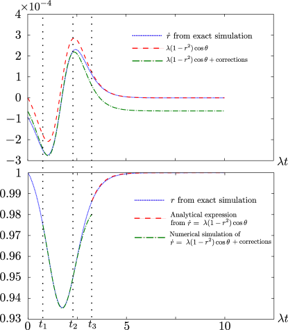
Figure 2: Comparison between the evolution of the polarization $r(t)$ by brute force numerical simulation of the quantum channel and the analytical solution. Four regions appear. The initial drop ($t<t_{1}$) and the crossover region ($t_{2}<t<t_{3}$) are not described by the semiclassical eq. of motions and seems to require a full quantum treatment. On the contrary, the polarization decrease ($t_{1}<t<t_{2}$) and increase ($t_{3}<t$) are described very accurately by semiclassical equations.

IV Decoherence of a superposition of coherent states

In this section, we will describe the evolution of states that behave semiclassically, namely coherent states, before investigating the evolution of a superposition of such states. It will exhibit dephasing on a much shorter timescale than relaxation.

IV.1 Coherent states

Coherent states have maximal angular momentum along a certain axis. If this axis is in the $xz$ plane with polar angle $\theta$, the corresponding quantum state reads, in the $|\ell,m\rangle$ basis,

$$|\theta\rangle=e^{-iL_{y}\theta}|\ell,\ell\rangle\mbox{.}$$ (22)

The semiclassical equations of motion (16) indicate that coherent states will keep maximal polarization ($\forall t\;r(t)\sim 1$) and align themselves with the $z$ axis, rotating around the $y$ axis according to (20). Once again, the ratio $\lambda$ plays a crucial role as it sets the timescale of the alignment of the gyroscope with the $z$ axis, which is exponentially fast. Equation (20) describes the relaxation or thermalization of the gyroscope, a classical phenomenon governed by the semiclassical equation of motions. In the next paragraph, we will investigate a purely quantum phenomenon, dephasing, which typically acts on a much shorter timescale.

IV.2 Evolution of a coherent superposition of coherent states

Consider a gyroscope initially prepared in a superposition of coherent states $|\psi\rangle=a|\theta\rangle+b|\phi\rangle$. The evolution of the coherence terms can be computed by using the Kraus expression of the quantum channel given in Poulin and Yard (2007) and expressing operators acting on $|\theta\rangle$ (resp. $|\phi\rangle$) in the basis $\{L^{\theta}_{x},\,L^{\theta}_{z}\}$ (resp. $\{L^{\phi}_{x},\,L^{\phi}_{z}\}$). The following equation describes how the evolution reduces the coherence terms:

$$\langle\theta|\mathcal{E}\left(|\theta\rangle\langle\phi|\right)|\phi\rangle=\cos^{2}\frac{\theta-\phi}{2}-\frac{\cos\theta-\phi}{d}\\ +\frac{2\ell\langle S_{z}\rangle}{d^{2}}\left(\cos\theta+\cos\phi\right)-\frac{2\langle S_{z}\rangle-\cos^{2}\frac{\theta-\phi}{2}}{d^{2}}\mbox{.}$$ (23)

In the semiclassical limit, i.e., $d\gg 1$ the first term dominates, as confirmed by numerical simulations shown in Fig. 3 for $\phi=0$.

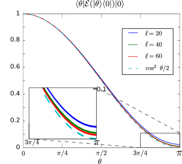
Figure 3: Evolution of the off-diagonal term $|\theta\rangle\langle 0|$ corresponding to the superposition $\alpha|\theta\rangle+\beta|0\rangle$ where $|0\rangle=|\ell,\ell\rangle$ points in the direction $z$ and $|\theta\rangle$ is given by equation (22)

Thus, the coherence terms vanish more and more rapidly as the initial value of $|\theta-\phi|$ increases. This is a feature similar to the result obtained for Quantum brownian motion Caldeira and Leggett (1983); Hu et al. (1992) where the coherence time of a superposition of two localized wavepackets is inversely proportional to the square of the distance Dávila Romero and Pablo Paz (1997). The difference of angles characterizes the classical distance between the two quasi-classical states.

The superposition $|\psi\rangle$ thus evolves according to

$$\mathcal{E}\left(|\psi\rangle\langle\psi|\right)=|a|^{2}|\theta+d\theta\rangle\langle\theta+d\theta|+|b|^{2}|\phi+d\phi\rangle\langle\phi+d\phi|\\ +ab^{*}\left(\cos^{2}\frac{\theta-\phi}{2}|\theta\rangle\langle\phi|+\chi\right)+\mbox{h.c.}$$ (24)

While eq. (23) gives the expression of a matrix element, eq. (24) is stronger since it represents a density matrix. However, we had to introduce an operator $\chi$, required by the trace-preserving nature of the channel $\mathcal{E}$. This operator accounts for terms that do not play a role in subsequent application of the channel evolution in the semiclassical limit $\ell\gg 1$ (see Fig. 4) as pointed out by numerical evidence shown on Fig. 4.

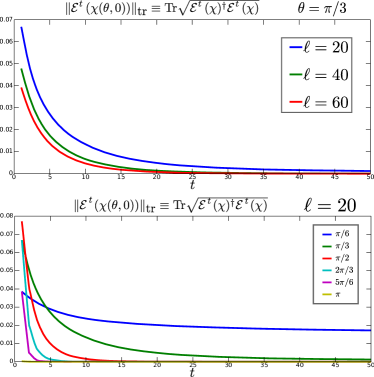
Figure 4: Numerical evolution of the trace norm of the operator $\chi$ with different values of $\ell$ for $\theta=\pi/3$ (top) and with different values of $\theta$ for $\ell=20$ (bottom). The norm vanishes, indicating that $\chi$ does not play a role in the evolution of the superposition of coherent states.

Thus, $|\psi\rangle\langle\psi|$ turns into a mixture $\sim|a|^{2}|\theta(t)\rangle\langle\theta(t)|+|b|^{2}|\phi(t)\rangle\langle\phi(t)|$ after interacting with a few incoming particles. This decoherence process is due to the entanglement with the incoming particles that allows the environment (made of all the incoming particles) to partially distinguish the two coherent components ($|\theta\rangle$ and $|\phi\rangle$) of the state. In the semiclassical limit $d\gg 1$, decoherence acts on a timescale that essentially depends on the “classical” distance $|\theta-\phi|$ and not on the semiclassical ratio $\lambda$ that governs relaxation. Indeed, unless the two coherent components are very close ($\theta\sim\phi$), decoherence acts exponentially fast, in the sense that $\langle\theta|\mathcal{E}\left(|\theta\rangle\langle\phi|\right)|\phi\rangle$ reduces to a value $\epsilon$ after interacting with a number of incoming particles that scales as $-\log\left(\cos^{2}\frac{\theta-\phi}{2}\right)$. Thus, in general, decoherence occurs on a timescale much shorter than relaxation. Once the two components $|\theta\rangle$ and $|\phi\rangle$ have decohered, they each relax and align with the $z$ axis independantly. These features are a revealing example of characteristics expected from the general theory of decoherence.

V Loss of purity

The predictability sieve, introduced in Zurek et al. (1993), identifies semiclassical states as those which minimize entropy production or purity loss. In the same way that minimal uncertainty coherent states are semiclassical for quantum Brownian motion Zurek et al. (1993), in our model, the $SU(2)$ coherent states clearly behave semiclassically and should minimize purity loss.

Interestingly, they still undergo a significant purity loss initially. After a few interactions, the gyroscope will lose a small amount of polarization, i.e. $r(t)=1-\varepsilon$ where $\varepsilon$ is small for large $l$. The resulting state $\rho$ will then be roughly a statistical mixture of $\varepsilon d$ states among the $d$ available states. Supposing that each coefficient has the same order of magnitude, the purity $\mbox{Tr}\rho^{2}$ will scale as $\varepsilon d(\frac{1}{\varepsilon d})^{2}=\frac{1}{\varepsilon d}$, explaining the loss of purity. This prediction agrees with numerical results (Fig. 5).

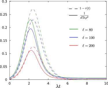
Figure 5: Evolution of the the purity $\mbox{Tr}\rho^{2}(t)$ for increasing values of $\ell$. Dashed lines represent the loss of polarization $\epsilon=1-r$ and the solid lines represent the inverse of $d\mbox{Tr}\rho^{2}$. Before the loss of polarization reaches a maximum, solid and dashed lines agree for all values of $\ell$.

VI Induced POVM

Interaction between the quantum gyroscope $\mathcal{R}$ and the spin-$\frac{1}{2}$ particle, which can be represented by a unitary operator $U=e^{-i\mathcal{H}_{\mathcal{RS}}\tau}$, creates an entangled state. Therefore, a measurement represented by a POVM $\{\Pi_{\pm}\}$ on the particle yields information about the state of the gyroscope according to the POVM $\{\Lambda_{\pm}\}$

$$\Lambda_{\pm}=\mbox{Tr}_{\mathcal{S}}\left[(\mathbb{I}_{\mathcal{R}}\otimes\sqrt{\xi})U^{\dagger}(\mathbb{I}_{\mathcal{R}}\otimes\Pi_{\pm})U(\mathbb{I}_{\mathcal{R}}\otimes\sqrt{\xi})\right]$$ (25)

Our calculations show that a projective measurement of the spin-$\frac{1}{2}$ particle along an axis $\mathbf{u}$ yields

$$\Lambda_{\pm}=\frac{1}{2}\mbox{Tr}_{\mathcal{S}}\left[\Pi_{\pm}\xi\right]\mathbb{I}_{\mathcal{R}}\pm\left(\langle\mathbf{S}\rangle\times\mathbf{u}\right)\cdot\frac{\mathbf{L}}{\ell+\frac{1}{2}}$$ (26)

corresponding to a measurement of $\mathbf{L}$ along $\langle\mathbf{S}\rangle\times\mathbf{u}$.

A broader problem is to evaluate the POVM induced by $n$ spin-$\frac{1}{2}$ particles interacting one after the other with the gyroscope during a time $\tau$ and then measured collectively. It is not clear how much information about the quantum state $\rho$ of the gyroscope can be gained this way. It is possible that only information about a few global properties of $\rho$ can be extracted for large but finite $n$ thus making these properties good candidates for characteristics that emerge in the semiclassical limit and which correspond to macroscopic attributes of the gyroscope.

Acknowledgements

This work is partially funded by FQRNT and NSERC. We thank David Poulin for many stimulating discussions about the model and its link to decoherence, and Mychel Pineault for useful discussions.

References

- Bartlett et al. (2007) S. D. Bartlett, T. Rudolph, and R. W. Spekkens, Rev. Mod. Phys., 79, 555 (2007).
- Bartlett et al. (2006) S. D. Bartlett, T. Rudolph, R. W. Spekkens, and P. S. Turner, New Journal of Physics, 8, 58 (2006).
- Poulin and Yard (2007) D. Poulin and J. Yard, New Journal of Physics, 9, 156 (2007).
- Ahmadi et al. (2010) M. Ahmadi, D. Jennings, and T. Rudolph, Phys. Rev. A, 82, 032320 (2010).
- (5) O. Landon-Cardinal and R. MacKenzie, “Poster presentation at the twelfth workshop on quantum information processing (qip), january 2009.” .
- Imamoḡlu et al. (2003) A. Imamoḡlu, E. Knill, L. Tian, and P. Zoller, Phys. Rev. Lett., 91, 017402 (2003).
- Coish and Loss (2004) W. Coish and D. Loss, Phys. Rev. B, 70, 1 (2004), ISSN 1098-0121.
- Cucchietti et al. (2005) F. Cucchietti, J. Paz, and W. Zurek, Phys. Rev. A, 72 (2005), ISSN 1050-2947.
- Landon-Cardinal and MacKenzie (2009) O. Landon-Cardinal and R. MacKenzie, Phys. Rev. A, 80, 062319 (2009).
- Petta et al. (2008) J. R. Petta, J. M. Taylor, A. C. Johnson, A. Yacoby, M. D. Lukin, C. M. Marcus, M. P. Hanson, and A. C. Gossard, Phys. Rev. Lett., 100, 067601 (2008).
- Reilly et al. (2008) D. J. Reilly, J. M. Taylor, J. R. Petta, C. M. Marcus, M. P. Hanson, and a. C. Gossard, Science, 321, 817 (2008), ISSN 1095-9203.
- Vink et al. (2009) I. T. Vink, K. C. Nowack, F. H. L. Koppens, J. Danon, Y. V. Nazarov, and L. M. K. Vandersypen, Nat. Phys., 5, 764 (2009), ISSN 1745-2473.
- Xu et al. (2009) X. Xu, W. Yao, B. Sun, D. G. Steel, A. S. Bracker, D. Gammon, and L. J. Sham, Nature, 459, 1105 (2009).
- Caldeira and Leggett (1983) A. O. Caldeira and A. J. Leggett, Physica A: Statistical and Theoretical Physics, 121, 587 (1983), ISSN 0378-4371.
- Hu et al. (1992) B. L. Hu, J. P. Paz, and Y. Zhang, Phys. Rev. D, 45, 2843 (1992).
- Dávila Romero and Pablo Paz (1997) L. Dávila Romero and J. Pablo Paz, Phys. Rev. A, 55, 4070 (1997).
- Zurek et al. (1993) W. H. Zurek, S. Habib, and J. P. Paz, Phys. Rev. Lett., 70, 1187 (1993).