Breit-Wigner Enhancement Considering the Dark Matter Kinetic Decoupling

Abstract

In the paper we study the Breit-Wigner enhancement of dark matter (DM) annihilation considering the kinetic decoupling in the evolution of DM freeze-out at the early universe. Since the DM temperature decreases much faster (as $1/R^{2}$) after kinetic decoupling than that in kinetic equilibrium (as $1/R$) we find the Breit-Wigner enhancement of DM annihilation rate after the kinetic decoupling will affect the DM relic density significantly. Focusing on the model parameters that trying to explain the anomalous cosmic positron/electron excesses observed by PAMELA/Fermi/ATIC we find the elastic scattering $Xf\to Xf$ is not efficient to keep dark matter in kinetic equilibrium, and the kinetic decoupling temperature $T_{kd}$ is comparable to the chemical decoupling temperature $T_{f}\sim O(10)GeV$. The reduction of the relic density after $T_{kd}$ is significant and leads to a limited enhancement factor $\sim O(10^{2})$. Therefore it is difficult to explain the anomalous positron/electron excesses in cosmic rays by DM annihilation and give the correct DM relic density simultaneously in the minimal Breit-Wigner enhancement model.

I Introduction

The recent cosmic ray observations by PAMELApamela-e , ATICatic and Fermifermi have all reported an excess of positrons and electrons from $\sim 10$ GeV up to $\sim 1$ TeV. These anomalies have stimulated a lot of interests, especially these excesses may be attributed to the signals of dark matter annihilation in the Galaxy. If these extra positrons/electrons are indeed from DM annihilation, it requires definite properties of DM. For example, DM should annihilate into lepton final states dominantly and should have a much larger annihilation cross section ($\langle\sigma v\rangle\sim 10^{23}$cm³s^-1) than the natural value ($\langle\sigma v\rangle\sim 10^{-26}$cm³s^-1) at freeze out Cirelli:2008pk ; Yin:2008bs ; Liu:2009sq . The annihilation cross section at freeze out determines the DM relic density if DM is generated thermally at the early universe.

In general, the DM annihilation cross section $\langle\sigma v\rangle$ depends on the averaged velocity of DM. For example, in the usual weakly interacting massive particle (WIMP) scenario, $\langle\sigma v\rangle$ can be expanded to a form of $a+b\langle v^{2}\rangle+O(v^{4})$ at the non-relativistic limit early . If the annihilation process is s-wave dominant, $\langle\sigma v\rangle$ is a constant. For the p-wave annihilation, $\langle\sigma v\rangle$ is proportional to $\langle v^{2}\rangle$. Therefore the DM annihilation by p-wave is suppressed today than the decoupling time since the WIMP usually has a velocity of $v\sim 10^{-1}$ at the freeze-out epoch and cools when universe expands. The DM velocity near the solar system is $v\sim 10^{-3}$, much smaller than that at the decoupling epoch.

However, as indicated by the PAMELA, ATIC and Fermi data, we actually ask for a much larger annihilation cross section today to account for the excesses than that at the early universe. Contrary to the analysis before for the p-wave annihilation we require an annihilation form $\langle\sigma v\rangle$ depends on $\sim 1/v^{n}$. This form leads to a large annihilation cross section today with low DM velocity and explains the cosmic positron anomaly and relic density simultaneously. Some mechanisms are soon proposed to achieve this aim after these results published, such as the Sommerfeld enhancement sommerfeld ; ArkaniHamed:2008qn and the Breit-Wigner enhancement Griest:1990kh ; Gondolo:1990dk ; Ibe:2008ye ; Guo:2009aj ; Bi:2009uj .

For the Sommerfeld enhancement, a new light mediator with mass of O(GeV) is introduced, and provide an enhancement factor of $S\sim\pi\alpha_{X}/v$ ($\alpha_{X}$ is coupling constant between DM and mediator). For the Breit-Wigner enhancement, the DM annihilates via a narrow resonance, and an enhance factor of $S\sim max[\delta,\gamma]^{-1}/O(10)$ can be obtained Ibe:2008ye ($\delta$, $\gamma$ are defined as $\delta=(4m^{2}-M^{2})/4m^{2}$ and $\gamma=\Gamma/M$ respectively, where m is the mass of DM, M and $\Gamma$ are the mass and decay width of the resonance respectively). One can achieve correct enhancement factor $S=\langle\sigma v\rangle_{{}_{T=0}}/\langle\sigma v\rangle_{{}_{T\sim T_{f}}}$ ($T_{f}$ is the temperature of chemical decoupling) by adjusting the parameters appropriately.

It seems that the enhancement should not be important in the early universe when the velocity of DM is $\sim O(10^{-1})$, and the enhancement factor is only $S\sim O(1)$. However, some recent studies showed that such effects are not negligible even at the freeze-out epoch Dent:2009bv ; Zavala:2009mi ; Feng:2009hw ; Feng:2010zp , especially for the Sommerfeld enhancement. The Ref. Feng:2009hw ; Feng:2010zp pointed out that it may be difficult to achieve the required enhancement factor in the minimal Sommerfeld models considering the effect at the early universe.

In this work, we will give a careful inspection on the Breit-Wigner mechanism at the DM freeze-out process. For the Breit-Wigner mechanism, the DM annihilation continues after the chemical decoupling until the DM velocity drops below the cut-off scale. Therefore the relic density is determined by the cut-off scale related to $\delta$ and $\gamma$ Bi:2009uj . In the work we will show another important factor in determining the relic density, i.e. the kinetic decoupling process Chen:2001jz ; Hofmann:2001bi ; Bringmann:2006mu .

After the chemical decoupling at $x\sim 20$ ($x$ represents the temperature of the universe which is defined as $x=m/T$), the DM particle is still kept in kinetic equilibrium via the scattering with the hot bath. When such scattering is not efficient to keep DM in kinetic equilibrium, the DM momentum is red-shifted with the scale factor $R$, which leads to a rapid decrease of DM temperature as $T_{X}\sim R^{-2}$ rather than $T_{X}\sim R^{-1}$ at the kinetic equilibrium epoch Chen:2001jz ; Hofmann:2001bi ; Bringmann:2006mu . Therefore, after the kinetic decoupling $\langle\sigma v\rangle$ increases quickly and then reduces the abundances of DM more efficiently. Taking this effect into account we find the Breit-Wigner mechanism is hard to provide a self-consistent explanation for both the DM relic density and the positron anomaly today.

This paper is organized as following. In Section II, we briefly describe the Breit-Wigner enhancement mechanism at the DM freeze-out epoch. In Section III, we discuss the kinetic decoupling process. We will calculate the kinetic decoupling temperature and the DM relic density including such effect. In Section IV, we investigate the enhancement factor required by the cosmic positron measurements. We will study the parameter space and discuss whether there exists such parameters to explain all the observations. Finally we give our conclusions and discussions in Section V.

II the Breit-Wigner enhancement

In Ref. Ibe:2008ye , the DM annihilation process is assumed through $X\bar{X}\to R\to f\bar{f}$, where $R$ is a narrow resonance with mass $M=\sqrt{4m^{2}(1-\delta)}$ and decay width $\Gamma=M\gamma$ with $|\delta|,\gamma\ll 1$. For a scalar resonance, the annihilation cross section is given as,

$$\sigma=\frac{16\pi}{M^{2}\bar{\beta}_{i}\beta_{i}}\frac{\gamma^{2}}{(\delta+v^{2}/4)^{2}+\gamma^{2}}B_{i}B_{f},$$ (1)

where $\bar{\beta}_{i}$ and $\beta_{i}$ are defined as $\sqrt{1-4m^{2}/M^{2}}$ and $1-4m^{2}/s$ respectively, $s$ is given by $s=(p_{1}+p_{2})^{2}$, $B_{i}$ and $B_{f}$ denote the branching fractions of the resonance into initial and final states respectively, $v$ is the relative velocity of two initial particles. For $\delta>0$, there exists an un-physical pole, but $B_{i}/\bar{\beta}_{i}$ is well defined. For simplicity, we parameterize the cross section as Ibe:2008ye

$$\sigma v=\sigma_{{}_{0}}\frac{\delta^{2}+\gamma^{2}}{(\delta+z)^{2}+\gamma^{2}}.$$ (2)

Here $\sigma_{{}_{0}}=\sigma v|_{{}_{T=0}}$ means the cross section at zero temperature limit which is velocity independent, and is set as a free parameter in our work . $z$ is defined in the form of $s\equiv 4m^{2}(1+z)$ which equals $v^{2}/4$ in the non-relativistic limit.

In order to calculate the DM relic density, it is necessary to solve the Boltzmann equation early

$$\frac{dY}{dx}=-\lambda^{\prime}x^{-2}\langle\sigma v\rangle(Y^{2}-Y^{2}_{eq})$$ (3)

where $Y=n_{\text{DM}}/s$ is the DM number density normalized by the entropy density $s$, $\lambda^{\prime}$ is defined as $\lambda^{\prime}=\frac{s}{H}|_{{}_{x=1}}$. The entropy density $s(x)$ and the Universe expansion rate $H(x)$ of the universe are given by

$$s(x)=\frac{2\pi^{2}g_{*S}}{45}\frac{m^{3}}{x^{3}}\;\;,\;H(x)=\sqrt{\frac{4\pi^{3}g_{*}}{45m_{pl}^{2}}}\frac{m^{2}}{x^{2}}\;,$$ (4)

where $g_{*}$($g_{i}$) is the effective number of degrees of freedom for radiations (DM), and $g_{*S}$ is the effective number of degrees of freedom defined by the entropy density. The $\langle\sigma v\rangle$ can be parameterized as $\langle\sigma v\rangle=\sigma_{{}_{0}}x^{-n}$ and the chemical decoupling temperature is obtained as early

$$x_{f}\simeq ln\varepsilon-(n+1/2)ln(ln\varepsilon),$$ (5)

where $\varepsilon\equiv c(c+2)a\lambda$ ($c\sim 1$ is a constant), $\lambda\equiv\lambda^{\prime}\sigma_{{}_{0}}$, and $a=0.145(g_{i}/g_{*})$ is defined in the form of $Y_{eq}=ax^{3/2}e^{-x}$ at low temperature. The final $Y$ as $x$ tends to $\infty$ could be obtained approximately as $Y_{\infty}\simeq(n+1)x_{f}^{n+1}/\lambda$ , and then the relic density $\Omega_{X}h^{2}=2.74\times 10^{8}\frac{m}{GeV}Y_{\infty}$.

In Ref. Ibe:2008ye , after parameterizing $\langle\sigma v\rangle$ for $\delta>0$, the Boltzmann equation could be rewritten as,

$$\frac{dY}{dx}=-\frac{\lambda}{x^{2}}\frac{\delta^{2}+\gamma^{2}}{(\delta+\xi x^{-1})^{2}+\gamma^{2}}(Y^{2}-Y^{2}_{eq}),$$ (6)

where $\xi\approx 1/\sqrt{2}$ is a constant (in fact, there is an assumption here that $x\sim v^{-2}$ or DM stays in kinetic equilibrium until very low temperature in Eq. (6)). For the Breit-Wigner enhancement, the freeze-out process begins at $\tilde{x}_{f}\sim O(10)$ , and continues until the temperature of $x_{b}\simeq max[\delta,\gamma]^{-1}$ when the DM annihilation cross section does not increase with the universe cooling. The final value of $Y$ is $Y_{\infty}\simeq x_{b}/\lambda$. In the ordinary S-wave non-resonant annihilation scenario with $\langle\sigma v\rangle=constant$, one could obtain $Y_{\infty}\simeq x_{f0}/\lambda_{0}$, where $x_{f0}\sim 20$, $\lambda_{0}\simeq\lambda^{\prime}\times 10^{-9}GeV^{-2}$. Then the enhancement factor is achieved as $S\simeq x_{b}/x_{f0}\simeq max[\delta,\gamma]^{-1}/O(10)$ Ibe:2008ye . The Breit-Wigner enhancement has been used to explain the anomalous positron excesses which require an enhancement factor of $\sim O(10^{3})$.

III Kinetic Decoupling of DM particles

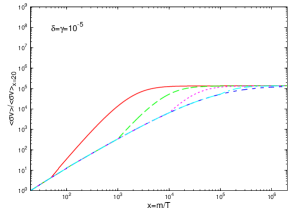
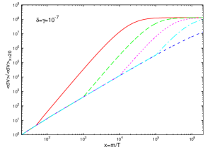
Figure 1: The Breit-Wigner enhanced relative cross section $\langle\sigma v\rangle/\langle\sigma v\rangle|_{{}_{x}=20}$ as a function of $x$. The curves in the figures from left to right denote $x_{{}_{kd}}=50,10^{3},10^{4},10^{5},\infty$ respectively. The model parameters in the figures from left to right are set as $\gamma=\delta=10^{-2},10^{-5},10^{-7}$ respectively.

In the early universe, the DM production and annihilation processes $X\bar{X}\rightleftharpoons f\bar{f}$ are efficient to keep DM particles in chemical and kinetic equilibrium. After chemical decoupling at $T_{f}$ DM may keep in kinetic equilibrium by momentum exchange with the hot bath of the standard model particles via the t-channel scattering $Xf\to Xf$, until the temperature decreases to the kinetic decoupling temperature $T_{kd}$.

Before kinetic decoupling, the DM has the same temperature as the thermal bath. After kinetic decoupling, the temperature of DM $T_{X}$ decreases as $1/R^{2}$, while the the temperature of thermal radiation still decrease as $1/R$. So the $T_{X}$ could be determined as Chen:2001jz ; Hofmann:2001bi ; Bringmann:2006mu

$$\left\{\begin{array}[]{cc}T_{X}=T,\;\;\;T_{X}>T_{kd}\\ \;\;\;\;T_{X}=T^{2}/T_{kd},\;\;\;T_{X}\leq T_{kd}\end{array}\right..$$ (9)

Since $T_{X}$ is different from $T$ one can define a parameter $x_{{}_{X}}$ related to DM temperature $T_{X}$ as

$$x_{{}_{X}}=\frac{m}{T_{X}}=\frac{2}{v_{0}^{2}},$$ (10)

where $v_{{}_{0}}$ is the most probable velocity of DM. The $\langle\sigma v\rangle$ is a function of $x_{{}_{X}}$ which is given by Gondolo:1990dk

$$\langle\sigma v\rangle=\frac{1}{n_{EQ}^{2}}\frac{m}{64\pi^{4}x_{{}_{X}}}\int_{4m^{2}}^{\infty}\hat{\sigma}(s)K_{1}(\frac{x_{{}_{X}}\sqrt{s}}{m})ds\;,$$ (11)

with

$$n_{EQ} = \frac{g_{i}}{2\pi^{2}}\frac{m^{3}}{x_{{}_{X}}}K_{2}(x_{{}_{X}})\;,$$ (12)

$$\hat{\sigma}(s) = 4E_{1}E_{2}\sigma vg_{i}^{2}\sqrt{1-\frac{4m^{2}}{s}}\;,$$ (13)

where $K_{1}(x)$ and $K_{2}(x)$ are the modified Bessel functions of the first and second type respectively.

After kinetic decoupling, the temperature of DM decreases rapidly, and the Breit-Wigner enhancement increases significantly. In the Fig. 1, we show the enhancement factor of $\langle\sigma v\rangle/\langle\sigma v\rangle|_{{}_{x}=20}$ for $x_{{}_{kd}}=50,10^{3},10^{4},10^{5}$ respectively. We also give the results in the limit of $x_{{}_{kd}}=\infty$ which denotes no kinetic decoupling. From Fig. 1, we can see the $\langle\sigma v\rangle$ for $x_{{}_{kd}}=50$ increases more quickly reaching the maximal value than the cases without kinetic decoupling. On the other hand, for a large value of $x_{{}_{kd}}=10^{4},10^{5}$, such effects are not very obvious. These results could be understood easily from Eq. (2) by assuming $\langle\sigma v\rangle\sim\sigma v|_{z\to v_{0}^{2}}$ roughly. When $x>x_{{}_{kd}}$ and $v_{0}^{2}\gg\delta,\gamma$, $\langle\sigma v\rangle$ increase as $x^{2}/x_{{}_{kd}}$ rather than $x$, and reaches $\sigma_{0}$ more quickly for small $x_{{}_{kd}}$.

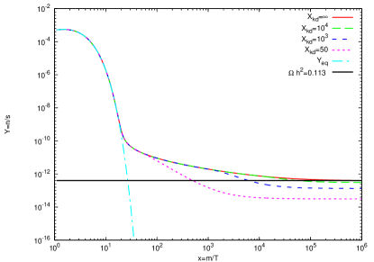
Figure 2: The evolution of DM abundance $Y$ as a function of $x$. The $x_{{}_{kd}}$ are taken as $50,10^{3},10^{4},\infty$ respectively.

The Fig. 2 shows the effects of kinetic decoupling in the calculation of the relic density. After kinetic decoupling, the annihilation of DM becomes more significantly, and reduce the relic density more efficiently. If kinetic decoupling is very late $x_{{}_{kd}}\gg\tilde{x}_{f}$, for example $x_{{}_{kd}}=10^{4}$, such effect is not very important compared with the case without kinetic decoupling. However, if the kinetic decoupling occurs at nearly the same epoch as the chemical decoupling, the efficient annihilation would reduce DM relic density by about one order of magnitude. Therefore the kinetic decoupling temperature $T_{kd}$ is a very important parameter in the calculation of the DM relic density.

The kinetic decoupling temperature $T_{kd}$ can be determined using the method in Refs. Feng:2010zp ; Hofmann:2001bi . If the momentum transfer rate drops below the expansion rate, the DM decouples from the kinetic equilibrium with the radiation background. Therefore, the $T_{kd}$ can be determined approximately by the relation of $\Gamma_{k}(T_{kd})=H(T_{kd})$. The momentum transfer rate is defined as Ref. Feng:2010zp ; Hofmann:2001bi

$$\Gamma_{k}\sim n_{r}\langle\sigma v\rangle_{s}\frac{T}{m}$$ (14)

where $n_{r}$ is the number density of massless fermions with $n_{r}=\frac{3}{4}\cdot\frac{1.202}{\pi^{2}}g_{f}T^{3}$, $\langle\sigma v\rangle_{k}$ is the thermally averaged cross section for the scattering process $Xf\to Xf$. Note that there exists a factor of $T/m$ in the above formula, which reflects the approximate momentum transfer at each collision.

Since the elastic scattering $Xf\to Xf$ via t-channel is suppressed by the propagator of $R$ with $1/(t-M^{2})^{2}\sim 1/M^{4}$, the cross section of this process is much smaller than the annihilation cross section. The explicit formula of the cross section for $Xf\to Xf$ depends on the model details. An approximate cross section of $Xf\to Xf$ is related to $X\bar{X}\to f\bar{f}$ as

$$\sigma v_{s}\sim a_{s}\sigma_{{}_{0}}(\delta^{2}+\gamma^{2})\frac{T^{2}}{m^{2}}\;\;,$$ (15)

where $a_{s}\leq O(1)$ is a constant determined by the form of the interaction (for more details, see the appendix). Then we can estimate $T_{kd}$ by setting $\Gamma_{k}(T_{kd})=H(T_{kd})$. Then we get

$$T_{kd} \sim 2.0\left[\frac{\sqrt{g_{{}_{*}}}m^{3}}{g_{f}a_{s}\sigma_{0}(\delta^{2}+\gamma^{2})m_{{}_{pl}}}\right]^{\frac{1}{4}}$$ (16)

$$\sim 30.GeV\left[\frac{1}{a_{s}}\right]^{\frac{1}{4}}\left[\frac{10^{-6}GeV^{-2}}{\sigma_{{}_{0}}}\right]^{\frac{1}{4}}\left[\frac{\;10^{{}^{-9}}}{\delta^{2}+\gamma^{2}}\right]^{\frac{1}{4}}$$

$$\times \left[\frac{4}{g_{f}}\right]^{-\frac{1}{4}}\left[\frac{g_{{}_{*}}}{100}\right]^{\frac{1}{8}}\left[\frac{m}{1TeV}\right]^{\frac{3}{4}}\;\;.$$

From above estimation, we can see the typical $T_{kd}$ in the Breit-Weigner enhancement model is O(10)GeV, which is much larger than that in the ordinary WIMP model. For example, the $T_{kd}$ for neutralino in the SUSY model is only O(10)MeV Chen:2001jz ; Hofmann:2001bi .

If $T_{kd}$ in Eq. (16) is larger than the DM freeze-out temprature $T_{f}\sim m/\tilde{x}_{f}\sim m/20$, it means the elastic scattering becomes unimportant before the chemical decoupling. However, the DM particles are still kept in thermal equilibrium by the annihilation process $f\bar{f}\to XX$. Therefore $T_{{}_{kd}}$ should be defined as $min(T_{f},T_{kd}^{\prime})$, where $T_{kd}^{\prime}$ is determined by the elastic scattering as given in Eq. (16).

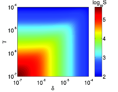
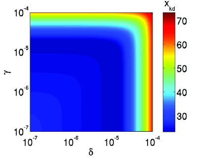
Figure 3: Numerical illustration of the DM annihilation enhancement factor $\sigma_{0}/\sigma_{nature}$ without considering kinetic decoupling effect (left) and the corresponding $x_{kd}$ (right) on the $\gamma-\delta$ plane.

For a more precise calculation, one need to derive the DM temperature $T_{{}_{X}}(T)$ from the Boltzmann equation

$$L[f]=C[f]\;\;,$$ (17)

where the $L$ and $C$ are Liouville operator and collision operator for the scattering process respectively. A general relation between the $T_{X}$ and $T$ has been provided by Ref. Bringmann:2006mu . In our work, we still adopt the simple relation between the $T_{X}$ and $T$ as Eq. (9), and use the formulae in Ref. Bringmann:2006mu to calculate the $T_{kd}^{\prime}$. We take a $Z^{\prime}$ model with $m_{DM}=1$TeV as an example, but our results can be extended to other models (for more details, see the appendix). From our calculations, we find that for the typical parameters used to explain the PAMELA/Fermi/ATIC results $x_{{}_{kd}}=m/T_{{}_{kd}}$ is not far from $\tilde{x}_{f}\sim O(10)$. To show this point explicitly, we give the boost factor $S=\sigma_{{}_{0}}/\sigma_{{}_{nature}}$ (left) and $x_{{}_{kd}}$ (right) for different $\delta$ and $\gamma$ in Fig. 3. Here $\sigma_{{}_{nature}}=3\times 10^{-26}$ cm³s^-1 is the so called ‘natural’ value of DM annihilation cross section predicted by the WIMP models to generate correct relic density. In the left plot, we require each point in the parameter space producing the correct relic density without kinetic decoupling effect, and determine the corresponding $\sigma_{{}_{0}}$. Then we use these $\delta$, $\gamma$ and $\sigma_{{}_{0}}$ to calculate $x_{{}_{kd}}$. We find in the parameter space favored by the PAMELA/Fermi/ATIC results with $S\sim O(10^{3})$, $x_{{}_{kd}}$ is similar as $\tilde{x}_{f}$. It means the kinetic decoupling effect should be important in the early universe when determining the DM relic density. Therefore it should be considered carefully in the explanation of the anomalous cosmic positron flux.

IV the enhancement factor for anomalous positron/electron flux

In this section, we calculate the enhancement factor by the Breit-Wigner resonance in the Galaxy today considering the kinetic decoupling. Here we define the enhancement factor as

$$S=\sigma_{{}_{G}}/\sigma_{{}_{nature}}\;\;,$$ (18)

where $\sigma_{{}_{G}}$ denotes the $\langle\sigma v\rangle$ of DM with the most probable velocity $v_{{}_{G}}\sim 10^{-3}$ in the Galaxy. This definition is different from the earlier form $s=\sigma_{{}_{0}}/\sigma_{{}_{nature}}$ Ibe:2008ye ; Guo:2009aj as the DM velocity is not zero today. We will see such difference is important.

We give the numerical results of $S$ in Fig. 4 and Fig. 5 for the cases of $\delta>0$ and $\delta<0$ respectively. For each point in the two figures, $\sigma_{0}$ has been adjusted to produce the correct relic density. The maximum value of $S$ is only $O(10^{2})$ with $\delta,\gamma\sim O(10^{-6})$ . From these results, we find the Breit-Wigner enhancement is difficult to provide large enough boost factor to explain the anomalous positron excesses after taking into account the kinetic decoupling effect.

To check this result analytically, one would turn to the discussion in the last paragraph of Sec. II Ibe:2008ye . After the kinetic decoupling, the $\xi x^{-1}$ in Eq. (6) should be modified by $\xi x_{kd}x^{-2}$. The DM annihilation would continue to the temperature of $x_{b}\sim max[\delta,\gamma]^{-\frac{1}{2}}\cdot\sqrt{x_{kd}}$. One can also obtain an enhancement factor as $S\sim x_{b}/x_{f0}\sim max[\delta,\gamma]^{-\frac{1}{2}}\cdot\sqrt{x_{kd}}/x_{f0}$. It seems we could still achieve a required boost factor by taking some smaller parameters such as $(\delta,\gamma)\sim O(10^{-(6\sim 8)})$. However, this is not the case. In fact, one can indeed obtain an arbitrary value of $\sigma_{{}_{0}}/\sigma_{{}_{nature}}$ by setting the $\delta$ and $\gamma$ tiny enough as discussed above. But the factor of $\sigma_{{}_{G}}/\sigma_{{}_{nature}}$ is different with that in the vanishing DM velocity limit. From the Eq. (2) we can see, for the parameters of $\delta\simeq\gamma\geq O(10^{-5})$, these two factors are equal, because the $\langle\sigma v\rangle$ always reaches its maximum value $\sigma_{{}_{0}}$ when the DM velocity decreases to $v_{{}_{G}}\sim z\sim 10^{-3}<max[\delta,\gamma]^{\frac{1}{2}}$. However, for $\delta\simeq\gamma<O(10^{-6})$, $\sigma_{{}_{G}}\sim\sigma_{{}_{0}}(max[\delta,\gamma]/v_{{}_{G}}^{2})^{2}$ is always smaller than $\sigma_{{}_{0}}$.

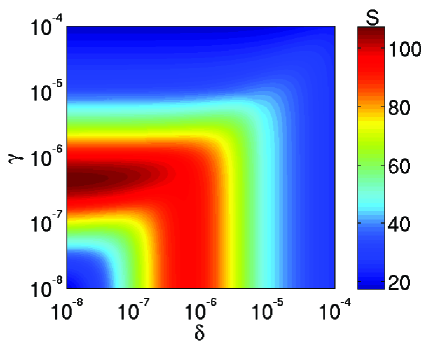
Figure 4: Numerical illustration of the enhance factor of $S=\sigma_{{}_{G}}/\sigma_{{}_{nature}}$ on the $\gamma-\delta$ plane for the $\delta>0$ case.

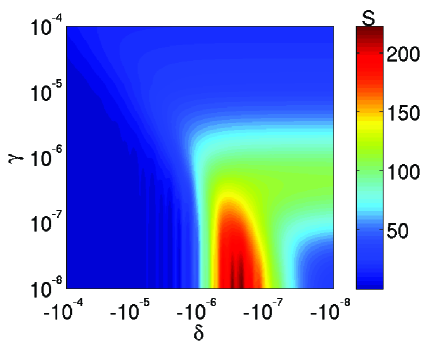
Figure 5: The same as Fig. 4 but for $\delta<0$.

To understand the maximum value of $\sigma_{{}_{G}}/\sigma_{{}_{nature}}$ and the corresponding parameters in Fig. 4 and Fig. 5, we can also use Eq. (2) as a roughly estimation. By setting $z\sim v_{{}_{G}}^{2}\sim 10^{-6}$ and $\sigma_{{}_{0}}/\sigma_{{}_{nature}}\sim max[\delta,\gamma]^{-\frac{1}{2}}\cdot\sqrt{x_{kd}}/x_{f0}$, we could obtain $S$

$$S\sim\frac{max[\delta,\gamma]^{\frac{3}{2}}}{max[\delta+v_{G}^{2},\gamma]^{2}}\cdot\frac{\sqrt{x_{kd}}}{x_{f0}}\;\;.$$ (19)

From this rough estimation, we can see for the $\delta>0$ case, there actually exists a maximum value of $S$ around $max[\delta,\gamma]\sim v_{G}^{2}\sim O(10^{-6})$ as shown in the Fig. 4. On the other hand, for the $\delta<0$, when $\gamma\gg\delta+v_{{}_{G}}^{2}\to 0$, the $S$ might be larger than the case of $\delta>0$. It means at the physical pole resonance, if the annihilations in the galaxy occur accurately with $v^{2}/4-\delta\to 0$, the cross section could be very large. However, considering the dispersion of the DM velocity our numerical results show the enhancement factor can not be very large either.

V Conclusion and Discussion

In this work, we study the Breit-Wigner enhancement for DM annihilation taking the kinetic decoupling effect at the early universe into account. We find if the kinetic decoupling occurs at nearly the same epoch as the chemical decoupling, the DM annihilation process becomes very important and reduces the DM relic density significantly. Requiring the model gives correct relic density we find there is no parameter space that can give an annihilation cross section today large enough to explain the anomalous cosmic positron/electron excesses at PAMELA/ATIC/Fermi.

The main point here is the elastic scattering between DM and massless fermions $Xf\to Xf$ is not efficient to maintain DM in thermal equilibrium. The kinetic decoupling occurs at high temperature $\sim T_{f}$. The DM temperature would decrease as $\sim T^{2}/T_{f}$ after kinetic decoupling, and reaches a very small value before the structure formation. For typical WIMP such as neutralino, the typical damping mass is $\sim 10^{-6}M_{\odot}(m/100GeV)^{-\frac{3}{2}}(T_{kd}/30MeV)^{-\frac{3}{2}}$ Bringmann:2006mu . Therefor in the Breit-Wigner enhancement with high $T_{kd}$, the damping mass might be much smaller than the usual cold DM model. This kind of DM model may predict tiny DM subhalo with $M_{{}_{sub}}\ll 10^{-6}M_{\odot}$ in the Galaxy. The realistic impact for the structure formation in the Breit-Wigner mechanism may need a careful study. This feature is possible to change the predictions for DM indirect detection.

Finally we would like to point out that it is still possible to explain the anomalous cosmic positron excesses in some non-minimal Breit-Wigner models. The ideal here is adding some new interaction process to keep DM in kinetic equilibrium till to a low temperature. For example, the DM is slepton $\tilde{\tau}$ in the hidden sector Feng:2009mn . It might interact with the hidden photon with a large coupling constant, or scatter with the standard model leptons by exchanging hidden neutralino in resonance. The hidden slepton annihilation to leptons could be enhanced by a $Z^{\prime}$ resonance in the $U(1)_{L_{i}-L_{j}}$ model Bi:2009uj . With this setting to enhance the scattering process, it is possible to obtain a low $T_{kd}$, and recover all the discussions in the earlier works about the Breit-Wigner mechanism.

Appendix A relation between cross sections of annihilation and elastic scattering processes

In this appendix, we would give detailed discussions about the relation between the cross sections of annihilation $X\bar{X}\to f\bar{f}$ and elastic scattering $Xf\to Xf$.

We assume the effective interaction Lagrangian between two DM particles (X) and two leptons (f) as

$$g_{A}g_{B}R_{0}\bar{X}\Gamma_{X}X\bar{f}\Gamma_{f}f$$ (20)

where $g_{A}$ and $g_{B}$ are interaction couplings of $X\bar{X}R$ and $f\bar{f}R$ respectively, $\Gamma_{X}$ and $\Gamma_{f}$ are combines of Lorentz metrics determined by model, $R_{0}$ is the propagator of resonance $R$. The cross section of annihilation process is (we neglect SM fermion mass $m_{{}_{f}}$ here)

$$\frac{d\sigma}{d\Omega}=\frac{1}{64\pi^{2}s}\sqrt{\frac{s}{s-4m^{2}}}g_{A}^{2}g_{B}^{2}|R_{0a}|^{2}|M^{\prime}_{a}|^{2}\;\;,$$ (21)

where we define the squared transition matrix element is $g_{A}^{2}g_{B}^{2}|R_{0a}|^{2}|M^{\prime}_{a}|^{2}$, $s,t,u$ are usual Mandelstam variables. For annihilation process in the non-relativistic limit, $s$ is approximated as $4m^{2}+m^{2}v^{2}$. So we can achieve $\sigma_{{}_{0}}$ as

$$\sigma_{{}_{0}}=\frac{1}{32\pi m^{2}}\frac{g_{A}^{2}g_{B}^{2}}{M^{4}(\delta^{2}+\gamma^{2})}\int\frac{|M^{\prime}_{a}|^{2}}{4\pi}d\Omega\;\;,$$ (22)

For the cross section of elastic scattering, we find

$$\sigma v_{s}=\frac{1}{16\pi m^{2}}\frac{g_{A}^{2}g_{B}^{2}}{M^{4}}\int\frac{|M^{\prime}_{s}|^{2}}{4\pi}d\Omega\;\;,$$ (23)

and the $\sigma v_{s}$ could be expressed by $\sigma_{{}_{0}}$ as

$$\sigma v_{s}=2\sigma_{{}_{0}}(\delta^{2}+\gamma^{2})\frac{\int|M^{\prime}_{s}|^{2}d\Omega}{\int|M^{\prime}_{a}|^{2}d\Omega}\;\;.$$ (24)

In general, the $|M^{\prime}_{a}|^{2}$ and $|M^{\prime}_{s}|^{2}$ are expressed by the four vector momentums of four particles. We define $p_{1}$, $p_{2}$ for two DM particles, and $k_{1}$, $k_{2}$ for two fermions. We need only calculate either one of $|M^{\prime}_{a}|^{2}$ and $|M^{\prime}_{s}|^{2}$, and make some modifications to obtain the other one. In the calculation, we can neglect all the sub-leading terms which are proportional to $m_{f}^{2}$, $v^{2}$, and assumed the energy of fermion in the scattering process is $\omega=3T/2$.

For example, we can calculate the relation between $\sigma v_{s}$ and $\sigma_{{}_{0}}$ in a $Z^{\prime}$ model with $\Gamma_{X}=\Gamma_{f}=\gamma^{\mu}$. The $|M^{\prime}_{a}|^{2}$ is given by

$$|M^{\prime}_{a}|^{2} = \frac{1}{4}\cdot 32\cdot[(k_{1}\cdot k_{2})m^{2}+(p_{1}\cdot k_{1})(p_{2}\cdot k_{2})$$ (25)

$$+ (p_{1}\cdot k_{2})(p_{2}\cdot k_{1})]=32m^{4}\;\;.$$

Then we can achieve $\overline{|M^{\prime}_{s}|^{2}}=8m^{2}\omega^{2}$ and $\sigma v_{s}=\frac{9}{8}\sigma_{{}_{0}}(\delta^{2}+\gamma^{2})\frac{T^{2}}{m^{2}}$.

Appendix B calculation for the kinetic decoupling temperature

In this appendix we show the calculation for the $T_{{}_{kd}}$ in a $Z^{\prime}$ model. The detailed method is described in Ref. Bringmann:2006mu , and can be extended to other models easily.

In general, the DM temperature $T_{{}_{X}}(T)$ can be derived by solving Boltzmann equation

$$T_{{}_{X}}=T\left[1-\frac{z^{\frac{1}{n+2}}}{n+2}exp[z]\Gamma[-(n+2)^{-1},z]\right]\;\;,$$ (26)

where $z=\frac{a}{n+2}(\frac{T}{m})^{n+2}$. In the low (high) temperature limit $T\to 0$ ($T\to\infty$), the $T_{{}_{X}}$ has the same form $T_{{}_{X}}\to T^{2}/m$ ($T_{{}_{X}}\to T$) as Eq. (9). Then the kinetic decoupling temperature can be obtained as

$$T_{{}_{kd}}=\left(\frac{T^{2}}{T_{{}_{X}}}\right)_{T\to 0}=m\left[\left(\frac{a}{n+2}\right)^{\frac{1}{n+2}}\Gamma\left[\frac{n+1}{n+2}\right]\right]^{-1}\;\;,$$ (27)

The parameters $a$ and $n$ are defined as follows. One need to expand the amplitude at $t=0$ and $s=m^{2}+2m\omega$

$$|M|^{2}=c_{n}\left(\frac{\omega}{m}\right)^{n}+O\left(\left(\frac{\omega}{m}^{n+1}\right)\right)\;\;,$$ (28)

The constant $a$ is given by

$$a=\sum_{f}\left(\frac{10}{(2\pi)^{9}g_{*}}\right)^{1/2}g_{f}c_{n}N_{n+3}^{\pm}\frac{m_{pl}}{m}\;\;.$$ (29)

The $N_{n+3}^{\pm}$ for fermion (plus sign) and scalar (minus sign) are given by

$$N_{n}^{\pm}=(1-p^{\pm}2^{-n})(n+1)!\zeta(n+1)\;\;,$$ (30)

where $p^{+}=1$ and $p^{-}=0$. For a $Z^{\prime}$ model with resonance mass $m_{Z^{\prime}}=M\sim 2m$ described as

$$\frac{g_{A}g_{B}}{M^{2}}\bar{X}\gamma^{\mu}X\bar{f}\gamma_{\mu}f\;\;,$$ (31)

we can achieve the amplitude at zero momentum transfer as $g_{A}^{2}g_{B}^{2}|M^{\prime}_{s}|^{2}_{t=0}/M^{4}=\frac{g_{A}^{2}g_{B}^{2}}{2}(\frac{\omega}{m})^{2}$. Substituting $n=2$ and $c_{2}=g_{A}^{2}g_{B}^{2}/2$ in the Eq. (27), we obtain $T_{{}_{kd}}$

$$T_{{}_{kd}}=1.326\left[\frac{\sqrt{g_{*}}m^{5}}{g_{f}c_{2}M_{{}_{pl}}}\right]^{\frac{1}{4}}\;\;.$$ (32)

Here we assume the $Z^{\prime}$ has the same couplings with the different leptons and sum the $g_{f}$ together. The thermal average annihilation cross section at low temperature can be written as $\sigma_{0}=c_{2}/8\pi m^{2}(\delta^{2}+\gamma^{2})$, the Eq. (33) can be re-written as

$$T_{{}_{kd}}=0.6\left[\frac{\sqrt{g_{*}}m^{3}}{g_{f}\sigma_{0}(\delta^{2}+\gamma^{2})M_{{}_{pl}}}\right]^{\frac{1}{4}}\;\;,$$ (33)

which is smaller than the result from Eq. (16) by a factor of O(1).

References

- (1) O. Adriani et al. [PAMELA Collaboration], Nature 458, 607 (2009).
- (2) J. Chang et al., Nature 456, 362 (2008).
- (3) A. A. Abdo et al. [The Fermi LAT Collaboration], Phys. Rev. Lett. 102, 181101 (2009).
- (4) M. Cirelli, M. Kadastik, M. Raidal and A. Strumia, Nucl. Phys. B 813, 1 (2009) [arXiv:0809.2409 [hep-ph]].
- (5) P. f. Yin, Q. Yuan, J. Liu, J. Zhang, X. j. Bi, S. h. Zhu and X. Zhang, Phys. Rev. D 79, 023512 (2009) [arXiv:0811.0176 [hep-ph]].
- (6) J. Liu, Q. Yuan, X. Bi, H. Li and X. Zhang, Phys. Rev. D 81, 023516 (2010) [arXiv:0906.3858 [astro-ph.CO]].
- (7) E. W. Kolb and M. S. Turner, The Early Universe, Westview Press (1994).
- (8) H. Baer, K. m. Cheung and J. F. Gunion, Phys. Rev. D 59, 075002 (1999) [arXiv:hep-ph/9806361]; J. Hisano, S. Matsumoto, M. M. Nojiri and O. Saito, Phys. Rev. D 71, 063528 (2005) [arXiv:hep-ph/0412403]; M. Cirelli, A. Strumia and M. Tamburini, Nucl. Phys. B 787, 152 (2007) [arXiv:0706.4071 [hep-ph]];
- (9) N. Arkani-Hamed, D. P. Finkbeiner, T. R. Slatyer and N. Weiner, Phys. Rev. D 79, 015014 (2009) [arXiv:0810.0713 [hep-ph]].
- (10) K. Griest and D. Seckel, Phys. Rev. D 43, 3191 (1991).
- (11) P. Gondolo and G. Gelmini, Nucl. Phys. B 360, 145 (1991).
- (12) M. Ibe, H. Murayama and T. T. Yanagida, Phys. Rev. D 79, 095009 (2009) [arXiv:0812.0072 [hep-ph]].
- (13) W. L. Guo and Y. L. Wu, Phys. Rev. D 79, 055012 (2009) [arXiv:0901.1450 [hep-ph]].
- (14) X. J. Bi, X. G. He and Q. Yuan, Phys. Lett. B 678, 168 (2009) [arXiv:0903.0122 [hep-ph]].
- (15) J. B. Dent, S. Dutta and R. J. Scherrer, Phys. Lett. B 687, 275 (2010) [arXiv:0909.4128 [astro-ph.CO]].
- (16) J. Zavala, M. Vogelsberger and S. D. M. White, Phys. Rev. D 81, 083502 (2010) [arXiv:0910.5221 [astro-ph.CO]].
- (17) J. L. Feng, M. Kaplinghat and H. B. Yu, Phys. Rev. Lett. 104, 151301 (2010) [arXiv:0911.0422 [hep-ph]].
- (18) J. L. Feng, M. Kaplinghat and H. B. Yu, arXiv:1005.4678 [hep-ph].
- (19) M. Backovic and J. P. Ralston, arXiv:1006.1885 [hep-ph].
- (20) J. L. Feng, M. Kaplinghat, H. Tu and H. B. Yu, JCAP 0907, 004 (2009) [arXiv:0905.3039 [hep-ph]].
- (21) X. l. Chen, M. Kamionkowski and X. m. Zhang, Phys. Rev. D 64, 021302 (2001) [arXiv:astro-ph/0103452].
- (22) S. Hofmann, D. J. Schwarz and H. Stoecker, Phys. Rev. D 64, 083507 (2001) [arXiv:astro-ph/0104173].
- (23) T. Bringmann and S. Hofmann, JCAP 0407, 016 (2007) [arXiv:hep-ph/0612238].