Starspots due to large-scale vortices in rotating turbulent convection

Abstract

We study the generation of large-scale vortices in rotating turbulent convection by means of Cartesian direct numerical simulations. We find that for sufficiently rapid rotation, cyclonic structures on a scale large in comparison to that of the convective eddies, emerge, provided that the fluid Reynolds number exceeds a critical value. For slower rotation, cool cyclonic vortices are preferred, whereas for rapid rotation, warm anti-cyclonic vortices are favored. In some runs in the intermediate regime both types of cyclones co-exist for thousands of convective turnover times. The temperature contrast between the vortices and the surrounding atmosphere is of the order of five per cent. We relate the simulation results to observations of rapidly rotating late-type stars that are known to exhibit large high-latitude spots from Doppler imaging. In many cases, cool spots are accompanied with spotted regions with temperatures higher than the average. In this paper, we investigate a scenario according to which the spots observed in the temperature maps could have a non-magnetic origin due to large-scale vortices in the convection zones of the stars.

1. Introduction

Rotating turbulent convection is considered to play a crucial role in the generation of large-scale magnetic fields (Moffatt, 1978; Krause & Rädler, 1980; Rüdiger & Hollerbach, 2004) and differential rotation of stars (Rüdiger, 1989). The interaction of rotation and inhomogeneous turbulence leads to the so-called $\alpha$-effect, which can sustain large-scale magnetic fields (e.g. Brandenburg, 2001; Käpylä et al., 2009). However, in many astrophysically relevant cases large-scale shear flows are also present, which further facilitate dynamo action by lowering the relevant critical dynamo number. In the Sun, for example, the entire convection zone is rotating differentially (cf. Schou et al., 1998; Thompson et al., 2003), and a meridional flow towards the poles is observed in the near surface layers (e.g. Zhao & Kosovichev, 2004). These flows are most often attributed to rotationally influenced turbulent angular momentum and heat transport (cf. Rüdiger, 1989; Robinson & Chan, 2001; Miesch et al., 2006; Käpylä et al., 2011b). In the solar case the large-scale flows and also the magnetic activity are largely axisymmetric (e.g. Pelt et al., 2006). This means that the sunspots, which are concentrations of strong magnetic fields, are almost uniformly distributed in longitude over the solar surface. The fact that we observe the sunspots and can attribute magnetic fields to them, has strongly influenced the interpretation of data from stars other than the Sun.

The giant planets Jupiter and Saturn are also likely to have outer convection zones (e.g. Busse, 1976), but they rotate much faster than the Sun. Bands of slower and faster rotation alternate in their atmospheres, reminiscent of rapidly rotating convection (e.g. Busse, 1994; Heimpel & Aurnou, 2007). However, especially in Jupiter, large spots in the form of immense storms are observed (Marcus, 1993). Remarkably, the largest of these, the Great Red Spot, has persisted at least 180 years. Similar features are observed also in Saturn (e.g. Sanchez-Lavega et al., 1991) and other giant planets. The spots on giant planets are not of magnetic origin although dynamos are likely to be present in the interiors of the planets. Thus their explanation is probably related to hydrodynamical processes within the convectively unstable layers.

Late-type stars with higher rotation velocities in comparison to the Sun, on the other hand, often exhibit light curve variations that are usually interpreted as large spots on the stellar surface (e.g. Chugainov, 1966; Henry et al., 1995). In some cases the observational data can be fitted with a model with two large spots at a 180 degree separation in longitude (Berdyugina & Tuominen, 1998). There is also evidence that these ‘active longitudes’ are not equal in strength (e.g. Lehtinen et al., 2011; Lindborg et al., 2011), and that the relative strength of the spots can, at least temporarily, reverse in a process dubbed ’flip-flop’ (cf. Jetsu et al., 1993). One interpretation of the data is that the spots are of magnetic origin and that the flip-flops are related to magnetic cycles reminiscent of the solar cycle (e.g. Berdyugina et al., 1998). On the other hand, it has been proposed that the flip-flops are only short-term changes related to the activity cycle, while the structure generating the temperature minima would migrate in the orbital reference frame. This can be interpreted as an azimuthal dynamo wave (e.g. Lehtinen et al., 2011; Lindborg et al., 2011). Again, this interpretation relies on the magnetic nature of the cool spots.

The cool spots detected by photometry and Doppler imaging using spectroscopic observations have been taken as an indirect proxy of the magnetic field on the stellar surface, deriving from the analogy to sunspots – strong magnetic field hinders convection and causes the magnetized region to be cooler than its surrounding. Zeeman-Doppler imaging of spectropolarimetric observations (e.g. Semel, 1989; Donati et al., 1989; Piskunov & Kochukhov, 2002; Carroll, 2007) provides means to directly measure the magnetic field strength and orientation on the stellar surface. In the study of Donati et al. (1997) spectropolarimetric observations of several stars were collected during 23 nights extending over a five year interval. They report that the Zeeman signatures of cool stars almost always exhibit a very complex shape with many successive sign reversals. This points to a rather complicated field structure with different magnetic regions of opposite polarities. Furthermore, these active regions were mostly 500 to 1,000 K cooler than, and sometimes at the same temperature as, but never warmer than the surrounding photosphere. In the published temperature and magnetic field maps for AB Dor (Donati & Collier Cameron, 1997), however, no clear correlation between temperature and magnetic field strength can be seen: in the temperature maps a pronounced cool polar cap with weak fringes towards lower latitudes are visible, whereas the strongest magnetic fields are seen as patchy structures at lower latitudes with a clearly different distribution in comparison to the temperature structures. Similar decorrelation of temperature minima and magnetic field strength has been reported with the same method for different objects (e.g. Donati, 1999; Jeffers et al., 2011), and also for the same objects with different methods (e.g. Hussain et al., 2000; Kochukhov et al., 2011). The phenomenon, therefore, seems to be wide-spread, and method-independent.

One possible explanation to the decorrelation of magnetic field and temperature structures could be that there is simply less light coming from the spotted parts than from the unspotted surface. Thus the Zeeman signatures from cool spots may be “drowned” in the signal from the unspotted surface or bright features. However, this should lead to systematic effects where the detected magnetic field strength would be correlated with the surface temperature. The least-squares deconvolution technique (e.g. Donati et al., 1997), which is necessary for enhancing the Zeeman signal, may influence the temperature and magnetic Doppler imaging differently. The latitudes of any surface features in Doppler images are always more unreliable than the longitudes, a fact that will not make a comparison of temperature and magnetic field maps any easier. One could thus expect, that there could be artificial discrepancies in the latitudes of magnetic and temperature features. Still, the lack of connection between even the longitudes of cool spots and magnetic features is surprising.

In this paper we consider a completely different scenario, according to which the formation of temperature anomalies on the surfaces of rapidly rotating late-type stars could occur due to a hydrodynamical instability generating large-scale vortices, analogously to the giant planets in the solar system. To manifest this mechanism in action, we simulate rotating turbulent convection in local Cartesian domains, representing parts of the stratified stellar convection zones located near the polar regions. We show that under such a setting, large-scale vortices or cyclones are indeed generated provided that the rotation is sufficiently rapid and the Reynolds number exceeds a critical value. Depending on the handedness of the vortex, which on the other hand depends on the rotation rate, the resulting spot can be cooler or warmer than the surrounding atmosphere.

We acknowledge that our model is rather primitive, lacking realistic radiation transport, spherical geometry, and relying on a polytropic setup for the stratification. Therefore, a detailed comparison with observations is not possible at this point. However, the main purpose of the present paper is to provide a proof of concept of the existence of large-scale vortices with temperature anomalies close to those observed in rapidly rotating hydrodynamic convection. We also note that similar large-scale cyclonic structures have recently been reported from large-eddy simulations of turbulent convection (Chan, 2003, 2007). We make comparisons to these studies when possible.

2. The model

Our model setup is the same as that used by Käpylä et al. (2009) but without magnetic fields. A rectangular portion of a star is modeled by a box situated at colatitude $\theta$. The box is divided into three layers: an upper cooling layer, a convectively unstable layer, and a stable overshoot layer (see below). We solve the following set of equations for compressible hydrodynamics:

$$\frac{\mathrm{D}\ln\rho}{\mathrm{D}t}=-\bm{\nabla}\cdot{\bm{U}},$$ (1)

$$\frac{\mathrm{D}\bm{U}}{\mathrm{D}t}=-\frac{1}{\rho}{\bm{\nabla}}p+{\bm{g}}-2\bm{\Omega}\times\bm{U}+\frac{1}{\rho}\bm{\nabla}\cdot 2\nu\rho\mbox{\boldmath${\sf S}$},$$ (2)

$$\frac{\mathrm{D}e}{\mathrm{D}t}=-\frac{p}{\rho}\bm{\nabla}\cdot{\bm{U}}+\frac{1}{\rho}\bm{\nabla}\cdot K\bm{\nabla}T+2\nu\mbox{\boldmath${\sf S}$}^{2}-\frac{e\!-\!e_{0}}{\tau(z)},$$ (3)

where $\mathrm{D}/\mathrm{D}t=\partial/\partial t+\bm{U}\cdot\bm{\nabla}$ is the advective time derivative, $\nu$ is the kinematic viscosity, $K$ is the heat conductivity, $\rho$ is the density, $\bm{U}$ is the velocity, $\bm{g}=-g\hat{\bm{z}}$ is the gravitational acceleration, and $\bm{\Omega}=\Omega_{0}(-\sin\theta,0,\cos\theta)$ is the rotation vector. The fluid obeys an ideal gas law $p=(\gamma-1)\rho e$, where $p$ and $e$ are the pressure and the internal energy, respectively, and $\gamma=c_{\rm P}/c_{\rm V}=5/3$ is the ratio of specific heats at constant pressure and volume, respectively. The specific internal energy per unit mass is related to the temperature via $e=c_{\rm V}T$. The rate of strain tensor ${\sf S}$ is given by

$${\sf S}_{ij}={\textstyle{1\over 2}}(U_{i,j}+U_{j,i})-{\textstyle{1\over 3}}\delta_{ij}\bm{\nabla}\cdot\bm{U}.$$ (4)

The last term of Eq. (3) describes cooling at the top of the domain. Here $\tau(z)$ is a cooling time which has a profile smoothly connecting the upper cooling layer and the convectively unstable layer below, where $\tau\to\infty$.

The positions of the bottom of the box, bottom and top of the convectively unstable layer, and the top of the box, respectively, are given by $(z_{1},z_{2},z_{3},z_{4})=(-0.85,0,1,1.15)d$, where $d$ is the depth of the convectively unstable layer. Initially the stratification is piecewise polytropic with polytropic indices $(m_{1},m_{2},m_{3})=(3,1,1)$, which leads to a convectively unstable layer above a stable layer at the bottom of the domain. In a system set up this way, convection transports roughly 20 per cent of the total flux (cf. Brandenburg et al., 2005). Due to the presence of the cooling term, a stably stratified isothermal layer forms at the top. The horizontal extent of the box, $L_{\rm H}\equiv L_{x}=L_{y}$, is $4d$. All simulations with rotation are made at the North pole, corresponding to $\theta=0\arcdeg$. The simulations were performed with the Pencil Code, which is a high-order finite difference method for solving the compressible equations of magnetohydrodynamics.

2.1. Units and non-dimensional parameters

Non-dimensional quantities are obtained by setting

$$d=g=\rho_{0}=c_{\rm P}=1\;,$$ (5)

where $\rho_{0}$ is the initial density at $z_{2}$. The units of length, time, velocity, density, and entropy are

$$[x]=d\;,\;\;[t]=\sqrt{d/g}\;,\;\;[U]=\sqrt{dg}\;,\;\;$$

$$[\rho]=\rho_{0}\;,\;\;[s]=c_{\rm P}.$$ (6)

We define the Prandtl number and the Rayleigh number as

$${\rm Pr}=\frac{\nu}{\chi_{0}}\;,\;\;{\rm Ra}=\frac{gd^{4}}{\nu\chi_{0}}\bigg{(}-\frac{1}{c_{\rm P}}\frac{{\rm d}s}{{\rm d}z}\bigg{)}_{0}\;,$$ (7)

where $\chi_{0}=K/(\rho_{\rm m}c_{\rm P})$ is the thermal diffusivity, and $\rho_{\rm m}$ is the density in the middle of the unstable layer, $z_{\rm m}={\textstyle{1\over 2}}(z_{3}-z_{2})$. The entropy gradient, measured at $z_{\rm m}$, in the non-convective hydrostatic state, is given by

$$\bigg{(}-\frac{1}{c_{\rm P}}\frac{{\rm d}s}{{\rm d}z}\bigg{)}_{0}=\frac{\nabla-\nabla_{\rm ad}}{H_{\rm P}}\;,$$ (8)

where $\nabla-\nabla_{\rm ad}$ is the superadiabatic temperature gradient with $\nabla_{\rm ad}=1-1/\gamma$, $\nabla=(\partial\ln T/\partial\ln p)_{z_{\rm m}}$, and where $H_{\rm P}$ is the pressure scale height. The amount of stratification is determined by the parameter $\xi_{0}=(\gamma-1)e_{0}/(gd)$, which is the pressure scale height at the top of the domain normalized by the depth of the unstable layer. We use $\xi_{0}=1/3$ in all cases, which results in a density contrast of about 23 across the domain. We define the Reynolds and Péclet numbers via

$${\rm Re}=\frac{u_{\rm rms}}{\nu k_{\rm f}}\;,\;\;{{\rm Pe}}=\frac{u_{\rm rms}}{\chi_{0}k_{\rm f}}=\Pr\ {\rm Re}\;,$$ (9)

where $k_{\rm f}=2\pi/d$ is adopted as an estimate for the wavenumber of the energy-carrying eddies, and $u_{\rm rms}=\sqrt{3u_{z}^{2}}$. This definition of $u_{\rm rms}$ neglects the contributions from the large-scale vortices that are generated in the rapid rotation regime. Note that with our definitions ${\rm Re}$ and ${\rm Pe}$ are smaller than the usual one by a factor of $2\pi$. The amount of rotation is quantified by the Coriolis number, defined as

$${\rm Co}=\frac{2\Omega_{0}}{u_{\rm rms}k_{\rm f}}\;.$$ (10)

We also quote the value of the Taylor number,

$${\rm Ta}=\left(2\Omega_{0}d^{2}/\nu\right)^{2},$$ (11)

which is related to the Ekman number via ${\rm Ek}={\rm Ta}^{-1/2}$.

2.2. Boundary conditions

The horizontal boundaries are periodic for all variables. Stress-free conditions are used for the velocity at the vertical boundaries.

$$U_{x,z}=U_{y,z}=U_{z}=0.$$ (12)

Temperature is kept constant on the upper boundary and the temperature gradient

$$\frac{dT}{dz}=\frac{-g}{c_{\rm V}(\gamma-1)(m+1)},$$ (13)

is held constant at the lower boundary, yielding a constant heat flux $F_{0}=-K\partial T/\partial z$ through the lower boundary.

Table 1Summary of the runs. Here, $\mbox{\rm Ma}=U_{\rm rms}/(gd)^{1/2}$ and $\mbox{\rm Ma}_{\rm z}=u_{\rm rms}/(gd)^{1/2}$. Brackets indicate that the simulation has not been run to a saturated state. The dimensionless input heat flux at the lower boundary of the box is given by $\tilde{F}_{0}=F_{0}/(\rho c_{\rm s}^{3})$, where $c_{\rm s}$ is the adiabatic sound speed and $\rho$ is the density, both measured at the lower boundary of the domain. The last column indicates the presence of cyclonic (C), anti-cyclonic (A), or both types (A+C) of vortices.

Run	grid	Ma	${\rm Ma}_{\rm z}$	${\rm Re}$	${\rm Pe}$	${\rm Pr}$	${\rm Ra}$	${\rm Co}$	Ta	$\tilde{F}_{0}$	Cyclones
A1	$256^{2}\times 128$	$0.048$	$0.020$	$33$	$8$	$0.24$	$2.0\cdot 10^{6}$	$15.5$	$4.0\cdot 10^{8}$	$1.7\cdot 10^{-5}$	yes (A)
A2	$256^{2}\times 128$	$0.018$	$0.017$	$13$	$6$	$0.48$	$1.0\cdot 10^{6}$	$14.4$	$5.6\cdot 10^{7}$	$1.7\cdot 10^{-5}$	no
A3	$256^{2}\times 128$	$0.022$	$0.019$	$21$	$7$	$0.36$	$1.3\cdot 10^{6}$	$12.3$	$1.0\cdot 10^{8}$	$1.7\cdot 10^{-5}$	no
A4	$256^{2}\times 128$	$(0.063)$	$0.023$	$37$	$9$	$0.24$	$2.0\cdot 10^{6}$	$10.3$	$2.3\cdot 10^{8}$	$1.7\cdot 10^{-5}$	yes (A)
A5	$256^{2}\times 128$	$0.021$	$0.020$	$16$	$9$	$0.48$	$1.0\cdot 10^{6}$	$7.9$	$2.5\cdot 10^{7}$	$1.7\cdot 10^{-5}$	no
A6	$256^{2}\times 128$	$0.024$	$0.023$	$24$	$9$	$0.36$	$1.3\cdot 10^{6}$	$7.0$	$4.4\cdot 10^{7}$	$1.7\cdot 10^{-5}$	no
A7	$256^{2}\times 128$	$(0.093)$	$0.026$	$42$	$10$	$0.24$	$2.0\cdot 10^{6}$	$6.1$	$1.0\cdot 10^{8}$	$1.7\cdot 10^{-5}$	yes (A+C)
A8	$256^{2}\times 128$	$0.028$	$0.027$	$28$	$11$	$0.36$	$1.3\cdot 10^{6}$	$3.6$	$1.6\cdot 10^{7}$	$1.7\cdot 10^{-5}$	no
A9	$256^{2}\times 128$	$0.082$	$0.028$	$45$	$11$	$0.24$	$2.0\cdot 10^{6}$	$3.4$	$3.6\cdot 10^{7}$	$1.7\cdot 10^{-5}$	yes (C)
A9b	$256^{2}\times 128$	$(0.070)$	$(0.031)$	$49$	$12$	$0.24$	$2.0\cdot 10^{6}$	$2.1$	$1.6\cdot 10^{7}$	$1.7\cdot 10^{-5}$	decay
A10	$256^{2}\times 128$	$0.032$	$0.033$	$53$	$13$	$0.24$	$2.0\cdot 10^{6}$	$1.0$	$4.0\cdot 10^{6}$	$1.7\cdot 10^{-5}$	no
A11	$256^{2}\times 128$	$0.038$	$0.038$	$61$	$15$	$0.24$	$2.0\cdot 10^{6}$	0	$0$	$1.7\cdot 10^{-5}$	no
B1	$256^{2}\times 128$	$0.017$	$0.016$	$26$	$13$	$0.48$	$4.0\cdot 10^{6}$	$9.7$	$1.0\cdot 10^{8}$	$8.6\cdot 10^{-6}$	no
B2	$256^{2}\times 128$	$(0.021)$	$(0.017)$	$37$	$13$	$0.36$	$5.4\cdot 10^{6}$	$9.1$	$1.8\cdot 10^{8}$	$8.6\cdot 10^{-6}$	yes (A+C)
B3	$256^{2}\times 128$	$(0.034)$	$(0.020)$	$63$	$15$	$0.24$	$8.0\cdot 10^{6}$	$8.0$	$4.0\cdot 10^{8}$	$8.6\cdot 10^{-6}$	yes (A+C)
C1	$256^{2}\times 128$	$0.011$	$0.011$	$17$	$16$	$0.96$	$8.0\cdot 10^{6}$	$14.8$	$1.0\cdot 10^{8}$	$4.3\cdot 10^{-6}$	no
C2	$256^{2}\times 128$	$(0.014)$	$(0.012)$	$25$	$18$	$0.72$	$1.1\cdot 10^{7}$	$13.6$	$1.8\cdot 10^{8}$	$4.3\cdot 10^{-6}$	no
C3	$256^{2}\times 128$	$(0.022)$	$(0.014)$	$44$	$21$	$0.48$	$1.6\cdot 10^{7}$	$11.6$	$4.0\cdot 10^{8}$	$4.3\cdot 10^{-6}$	yes (A)
D1	$256^{2}\times 128$	$0.013$	$0.013$	$42$	$51$	$1.20$	$4.0\cdot 10^{7}$	$7.2$	$1.4\cdot 10^{8}$	$1.7\cdot 10^{-6}$	no
D2	$512^{2}\times 256$	$(0.038)$	$(0.013)$	$101$	$49$	$0.48$	$1.0\cdot 10^{8}$	$7.5$	$9.0\cdot 10^{8}$	$1.7\cdot 10^{-6}$	yes (A+C)

3. Results

We perform a number of numerical experiments in order to determine the conditions under which large-scale cyclones are excited. The basic input parameters and some key diagnostic outputs of the simulations are listed in Table 1. We perform a few (Set A) or a single (Sets B, C, and D) progenitor run with a given input heat flux and approximately constant Péclet number in each Set from which the rest of the runs are obtained by continuing from a thermally saturated snapshot and changing the value of the kinematic viscosity $\nu$ in order to change ${\rm Re}$. The higher resolution run D2 was remeshed from a lower resolution case D1.

3.1. Excitation of large-scale vortices

We perform several sets of runs where the Péclet number and input energy flux are constant, whereas the Reynolds and Coriolis numbers are varied. We are limited to exploring a small number of cases due to the slow growth of the vortices, see Table 1. Typically the time needed for the saturation of the cyclones is several thousand convective turnover times (see Fig. 1). For Run A7 in Fig. 1, $tu_{\rm rms}k_{\rm f}\approx 4300$ corresponds to roughly $9\tau_{\rm ther}$ or $2.2\cdot 10^{4}\tau_{\rm dyn}$, where $\tau_{\rm ther}=d^{2}/\chi_{0}$ is the thermal diffusion time and $\tau_{\rm dyn}=\sqrt{d/g}$ is the dynamical free fall time. However, when the input flux is lowered, by decreasing the heat conductivity, the thermal relaxation time increases. For Runs D1 and D2 the thermal diffusion time is ten times longer than for runs in Set A. Thus many of our runs were continued only until the presence or the absence of the cyclones was apparent.

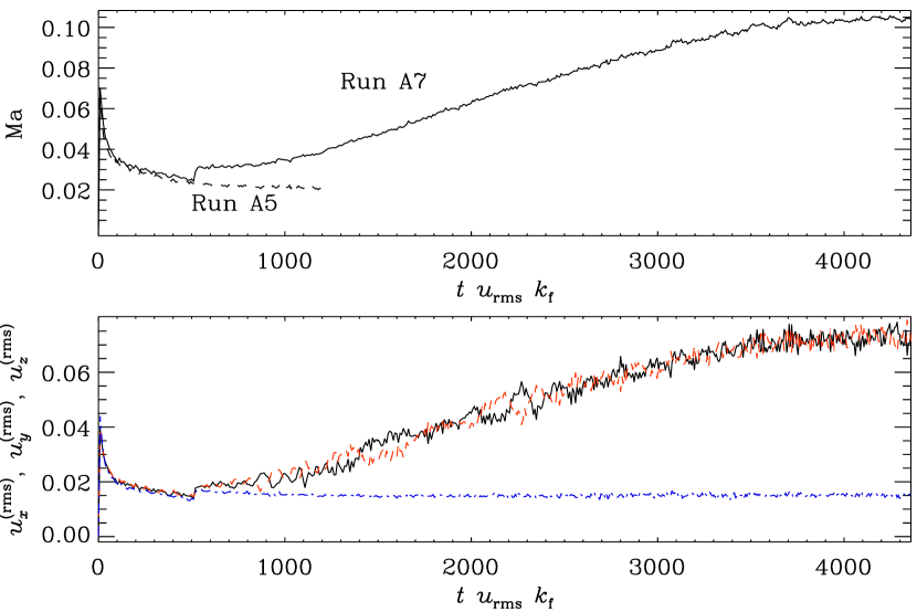
Figure 1.— Upper panel: total rms-velocity ${\rm Ma}=U_{\rm rms}/(dg)^{1/2}$ from Runs A5 and A7. Lower panel: velocity components $\sqrt{u_{x}^{2}}$ (black solid line), $\sqrt{u_{y}^{2}}$ (red dashed), and $\sqrt{u_{z}^{2}}$ (blue dot-dashed) from Run A7 in units of $(dg)^{1/2}$. The jump at $tu_{\rm rms}k_{\rm f}\approx 500$ is due to a lowering of $\nu$ at this point.

We find that a reliable diagnostic indicating the presence of large-scale vortices is to compare the rms-value of the total velocity, $U_{\rm rms}$, and the volume average of the quantity $u_{\rm rms}=\sqrt{3u_{z}^{2}}$. The latter neglects the horizontal velocity components, which grow significantly when large-scale cyclones are present (see the lower panel of Fig. 1). In the cyclone-free regime, irrespective of the rotation rate, we find that $U_{\rm rms}\approx u_{\rm rms}$ suggesting that the flow is only weakly anisotropic (see Table 1). In the growth phase of the vortices one of the horizontal velocity components is always stronger, but the relative strength of the components changes as a function of time (see the lower panel of Fig. 1). This undulation is related to quasi-periodic changes of the large-scale pattern of the flow, although their ultimate cause is not clear.

Another quantitative diagnostic is to monitor the power spectrum of the flow from a horizontal plane within the convection zone. A typical example is shown in Fig. 2 where power spectra of the velocity from the middle of the convection zone at two different times from Run B3 are shown. The snapshot at $tu_{\rm rms}k_{\rm f}=1830$ is the initial state for Run B3, taken from a lower Reynolds number Run B1, showing no cyclones. The power spectrum shows a maximum at $k/k_{1}=7$, indicating that most of the energy is contained in structures having a size typical of convective eddies. However, as the run is continued further, a large-scale contribution due to the appearance of the vortices, peaking at $k/k_{1}=1$ grows, and ultimately dominates the power spectrum. We note that this run was not continued until saturation so the peak at $k/k_{1}=1$ is likely to be even higher in the final state. The presence of the vortices is also clear by visual inspection of the flow. A typical example is shown in Fig. 3, where the vertical velocity component, $U_{z}$, is shown from the periphery of the domain for Run D2.

Figure 2.— Power spectra of velocity from early (dashed line) and late (solid) times from Run B3 from $z=z_{\rm m}$.

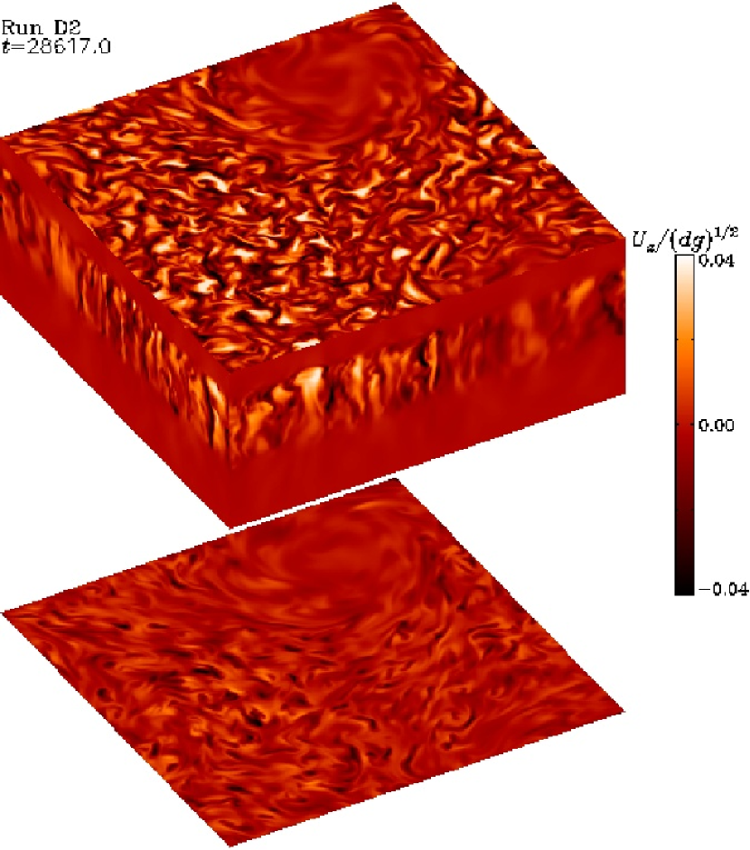
Figure 3.— Vertical velocity component $U_{z}$ at the periphery of the box from Run D2. See also http://www.helsinki.fi/$\sim$kapyla/movies.html. The top and bottom panels show slices near the top and bottom of the convectively unstable layer, respectively.

The data in Table 1 suggests that large-scale vortices are excited provided the Reynolds number exceeds a critical value, ${\rm Re}_{\rm c}$. For ${\rm Pe}\approx 10$ (Set A) we find that ${\rm Re}_{\rm c}$ is around 30, although the sparse coverage of the parameter range does not allow a very precise estimate to be made. We find a similar value for ${\rm Re}_{\rm c}$ in Sets B and C, whereas for ${\rm Pe}\approx 50$ in Set D, the critical Reynolds number is greater than 42. In Set C, Runs C1 and C2 were started from a snapshot of Run C3 at a time when vortices were already clearly developing. In both cases we find that the cyclones decay, suggesting that their presence is not strongly dependent on the history of the run.

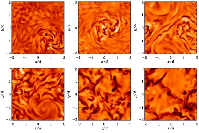
Figure 4.— From left to right: vertical velocity $U_{z}$ from $z=z_{\rm m}$ for Runs A1, A4, A7 (upper row), A9, A10, and A11 (lower row). The rotational influence is decreasing from left to right and top to bottom.

The critical Coriolis number in Set A is somewhere between 2.1 and 3.4. Again a very precise determination cannot be made, but continuing from a saturated snapshot of Run A9 with a somewhat lower rotation rate indicates that the vortices decay (Run A9b). We have limited the present study to the North pole ($\theta=0$), but vortices are also excited at least down to latitude $\theta=45\arcdeg$ (cf. Chan, 2007).

3.2. Thermal properties of the cyclones

In order to study the possible observable and other effects of the vortices, we ran a few simulations in Set A (Runs A1, A4, A7, A9, A10, and A11) to full saturation. Figures 4 and 5 show the vertical velocity and temperature in the saturated regime from the six runs listed above. In the non- and slowly rotating cases (the two rightmost panels on the lower rows of Figs 4 and 5), convection shows a typical cellular pattern. Vorticity is generated at small scales at the vertices of the convection cells, but no large-scale pattern arises. We note that long-lived large-scale circulation can also emerge in non-rotating convection (e.g. Bukai et al., 2009). However, such structures are not likely to be of relevance in rapidly rotating stars.

When the rotation is increased to ${\rm Co}\approx 3.4$, a cyclonic, i.e. rotating in the same sense as the overall rotation of the star, vortex appears (the lower left panels of Figs. 4 and 5). Vertical motions are suppressed within the vortex and it appears as a cool spot in the temperature slice. Increasing rotation further to ${\rm Co}\approx 6$, also an anti-cyclonic, i.e. rotating opposite to the overall fluid rotation, warm vortex appears (the rightmost upper panels of Figs. 4 and 5). In Run A7 the two vortices coexist for thousands of convective turnover times. In the most rapidly rotating cases A1 and A4 (the two leftmost panels in the upper rows of Figs. 4 and 5) a single anti-cyclonic vortex persists in the saturated regime. A similar behaviour as a function of rotation was found by Chan (2007) from large-eddy simulations. The anti-cyclonic vortices show vigorous convection whereas in the surrounding regions convection appears suppressed. Due to the enhanced energy transport by convection, the anti-cyclones appear as warmer structures than their surroundings in the temperature slices.

Figure 6 shows that in Runs A9 and A1 the flow is in geostrophic balance, i.e. that the flow follows the isocontours of pressure for both types of vortices. The cyclone in Run A9 appears as a low-pressure area, similarly to the cyclones in the atmosphere of the Earth, whereas the anti-cyclone in Run A1 coincides with a high pressure region. A weaker high pressure region is present also in Run A9. It is not clear whether this kind of single or two spot configuration lasts if the domain is larger in the horizontal directions, or whether a greater number of spots appear. We find that the temperature contrast between the spot and the surrounding medium is of the order of five per cent (Fig. 7) for both types of vortices. Although the relative temperature contrast between the vortex and the surrounding vortex-free convection seems to be a robust feature in the simulations, we must remain cautious when comparing the results with observations. This is due to the rather primitive nature of the simulations that lack realistic radiation transport. Convection in our model is also fairly inefficient by design, only 20 percent of the total flux being carried by it.

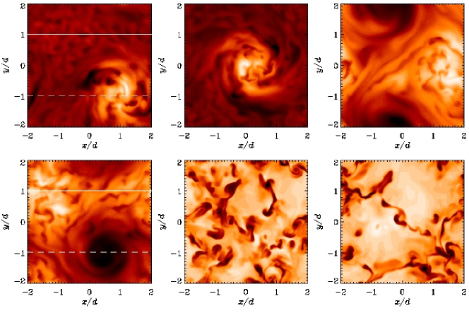
Figure 5.— From left to right: temperature from $z_{\rm m}$ for Runs A1, A4, A7 (upper row), A9, A10, and A11 (lower row). The rotational influence is decreasing from left to right and top to bottom. The solid and dashed horizontal lines on the leftmost panels correspond to line plots shown in Fig. 7.

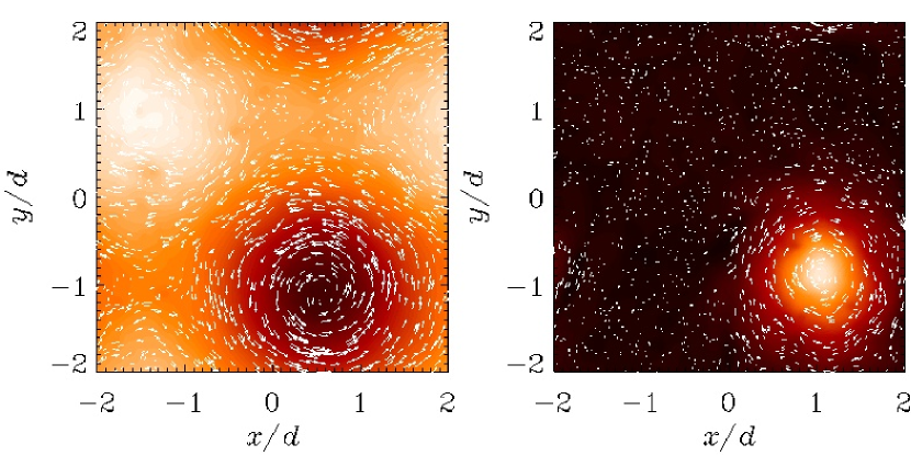
Figure 6.— Pressure (colors) and horizontal flows (arrows) from the middle of the convection zone in Runs A9 (left panel) and A1 (right panel).

3.3. Dynamo considerations and discussion

Figure 8 shows the horizontally averaged kinetic helicity, $\overline{\bm{\omega}\cdot{\bm{u}}}$, where $\bm{\omega}=\bm{\nabla}\times{\bm{u}}$, from Runs A9 and A1 from the initial, purely convective cyclone-free, and final fully saturated stages of the simulations. The data is averaged over a period of roughly 60 convective turnover times in each case. We find that in Run A9, where a cool cyclonic vortex appears, there is almost no change in the kinetic helicity between the initial and final stages of the simulation. In this run convection, and thus vertical motions, are largely suppressed within the vortex (see Fig. 4). Furthermore, the dominant contribution to the vorticity due to the cyclone arises via the vertical component $\omega_{z}=\partial_{x}u_{y}-\partial_{y}u_{x}$, which is positive for a cyclonic vortex. These two effects seem to compensate each other and the helicity within the cyclone is not greatly enhanced or depressed with respect to the surroundings. This would indicate that the influence of the cyclonic vortices on the magnetic field amplification would be minor, as the helicity remains unaltered. On the other hand, the strong horizontal motions connected to the cyclone might be able to amplify the field by advecting the field lines.

In Run A1, on the other hand, a more pronounced effect is seen, and the helicity is decreased up to a factor of two in the saturated stage (see the right panel of Fig. 8). This change is brought about by the different handedness of the vorticity in the anti-cyclone and by the vigorous convection within it (see the upper row of Fig. 4). The combination of these produces significantly greater helicity in the anti-cyclones, but a predominantly different sign than in the surroundings and leads to an overall decrease noted in Fig. 8. The decreased helicity suggests weaker amplification of the magnetic field by anti-cyclones compared to their surroundings. Again, the strong large-scale horizontal motions might counteract by amplifying the field by advection.

The simulations presented here were performed with a setup identical to that used in (Käpylä et al., 2009, hereafter KKB09) to study large-scale dynamo (LSD) action in rotating convection. In KKB09 the generation of large-scale magnetic fields, given that the Coriolis and magnetic Reynolds numbers exceeded critical values, were reported. The critical Coriolis number for LSD action was found to be roughly four, which is close to the critical value for the cyclones to emerge.

The relation of the two phenomena is an interesting question, that can be only partially answered by the existing magnetohydrodynamic runs from KKB09. This is because the fluid Reynolds number in the runs of KKB09 was in most cases lower than ${\rm Re}_{\rm c}$ required for the vortices to appear. Only two runs (A10 and D1 of KKB09) are clearly in the parameter regime exceeding the critical values found here, in addition to four runs (A5, A6, B5, and C1 of KKB09) where the parameters were close to marginal. The Reynolds and Coriolis numbers for these runs were calculated from the saturated state of the dynamo which in all cases lowers the turbulent velocities somewhat, decreasing ${\rm Re}$ and increasing ${\rm Co}$ correspondingly. Furthermore, a different definition of the Reynolds number was used by KKB09 than in the present study. A reanalysis of the data of KKB09 suggests that early stages of cyclone formation are in progress in all of the six runs listed above. However, the magnetic field grows on a significantly shorter timescale than the cyclones, and the magnetic field saturates already before thousand convective turnover times. None of the runs was continued much further than twice that, making it impossible to decide in favor or against the maintenance of vortices based on these runs.

Nonetheless, indications of growing cyclones appear in the kinematic regime, i.e. when the magnetic field is weak in comparison to the kinetic energy of the turbulence, but they are far less clear, or even absent, when the magnetic field saturates. This raises two related questions: firstly, are the vortices responsible for the emergence of the large-scale magnetic fields, and secondly, can the vortices coexist in the regime where strong magnetic fields are present? The current data suggests that the presence of the vortices is not essential for the large-scale magnetic fields which persist throughout the saturated state, whereas the vortices remain less prominent or suppressed. This fact is related to the second issue. As noted above, the simulations of KKB09 are too short for the vortices to fully saturate. Thus, we cannot conclusively state whether the lack of the vortices in the dynamo regime is due to the magnetic field simply reducing the Reynolds number below the critical value, or a direct influence of the Lorentz force on the growing vortices. We will address the questions related to magnetic fields and dynamo action in more detail in a forthcoming publication.

Figure 7.— Temperature as a function of $x$ from a quiescent (solid lines) and cyclonic (dashed) regions for Runs A9 (left panel) and A1 (right panel) from $z=z_{\rm m}$. The positions of the cuts are indicated in the leftmost panels of Fig. 5 with corresponding linestyles. The normalization factor $\overline{T}$ is the horizontal average of the temperature.

Figure 8.— Horizontally averaged kinetic helicity $\overline{\bm{\omega}\cdot{\bm{u}}}$ as a function of $z$ from a quiescent (solid lines) and cyclonic (dashed) states for Runs A9 (left panel) and A1 (right panel). The vertical dotted lines at $z=0$ and $z=d$ indicate the bottom and top of the convectively unstable layer, respectively.

3.4. Observational implications

If large-scale cyclones such as those found in the present study occur in real stars, they will cause observational signatures on the stellar surface due to their lower or higher temperatures. The temperature contrasts seen in the surface maps obtained by Doppler imaging are somewhat stronger than the value of roughly five percent found in this study; for instance, on the surface of the active RS CVn binary II Peg, analyzed by Lindborg et al. (2011) and Hackman et al. (2011), the coolest spot temperatures, depending on the season, are 10-20 per cent below the mean surface temperature. Similar spot temperatures have also been obtained by analyzing molecular absorption bands, but cooler stars seem to have a lower spot contrast (O’Neal et al., 1998). Taken that the numerical model is quite simple, for instance in the sense that the transport of energy by convection is underestimated, this discrepancy is not overwhelmingly large. Interestingly, Doppler images commonly also show hot surface features (cf. Korhonen et al., 2007; Lindborg et al., 2011; Hackman et al., 2011). These may be artefacts of the Doppler imaging procedure, but it is not ruled out that they could arise from real physical sources, such as the anti-cyclonic vortices seen in the present study.

It is obviously very hard to explain active longitudes and their drift based on the vortex instability scenario; we believe that a large-scale dynamo process is responsible for these basic features, as commonly believed (e.g. Krause & Rädler, 1980; Moss et al., 1995; Tuominen et al., 2002). Nevertheless, it is possible that the vortex-instability contributes to the formation of starspots, and may interfere with the dynamo-instability, especially during the epochs of lower magnetic activity of the stellar cycle. Although it is very hard to predict the implications of the vortices in the magnetohydrodynamic regime, it would appear natural that spots, either cool or warm, generated by a hydrodynamic vortex-instability, could also contribute to the apparent decorrelation of magnetic field from the temperature structures.

The net helicity, which is important for the amplification of the magnetic field, will be influenced differently by cyclones and anti-cyclones. Anti-cyclones will decrease the net helicity, while the effect of cyclones will be close to zero. This seems to imply that the magnetic field amplification would be equally or even more difficult in the regions of the vortices; this picture, however, may be complicated by the presence of strong large-scale horizontal motions present in these structures, that might amplify the magnetic field simply by their capability for advecting the field lines.

4. Conclusions

We report the formation of large-scale vortices in rapidly rotating turbulent convection in local f-plane simulations. The vortices appear provided the Reynolds and Coriolis numbers exceed critical values. Near the critical Coriolis number, the vortices are cyclonic and cool in comparison to the surrounding atmosphere, whereas for faster rotation warm anti-cyclonic vortices appear (see also Chan, 2007). The relative temperature difference between the vortex and its surroundings is of the order of five per cent in all cases. This is of the same order of magnitude as the contrast deduced indirectly from photometric and spectroscopic observations of late-type stars. In our simulations the typical size of the vortices is comparable to the depth of the convectively unstable layer. However, we have not studied how the size of the structures depends e.g. on the depth of the convection zone.

We propose that the vortices studied here can be present in the atmospheres of rapidly rotating late-type stars, thus contributing to rotationally modulated variations in the brightness and spectrum of the star. Such features have generally been interpreted to be caused by magnetic spots, reminiscent of sunspots. However, our results suggest that the turbulent convection and rapid rotation of these stars can generate large-scale temperature anomalies in their atmospheres via a purely hydrodynamical process. Similar vortex-structures are observed in the atmospheres of Jupiter and Saturn. Although their definitive explanation is still debated, it is possible that they are related to rapidly rotating thermal convection in their atmospheres.

However, several issues remain to be sorted out before the reality of cyclones and anti-cyclones in the surface layers of stars can be established. The current model is highly simplified and neglects the effects of sphericity and magnetic fields. In spherical geometry more realistic large-scale flows can occur which might lead to other hydrodynamical instabilities. However, current rapidly rotating simulations in spherical coordinates have not shown evidence of large-scale vortices (e.g. Brown et al., 2008; Käpylä et al., 2010, 2011b), although non-axisymmetric features are seen near the equator (Brown et al., 2008). It is possible that the lack of large-scale vortices in these simulations is related either to the lack of spatial resolution or too short integration time.

Magnetic fields, on the other hand, are ubiquitous in stars with convection zones. Furthermore, on the Sun they form strong flux concentrations, i.e. sunspots. At the moment, direct simulations cannot self-consistently produce sunspot-like structures in local geometry (e.g. Käpylä et al., 2011a). However, the magnetic fields in global simulations are also very different from the high-latitude spots and active longitudes deduced from observations, namely showing more axisymmetric fields residing also near the equator (e.g. Käpylä et al., 2010; Brown et al., 2011). The apparently poor correlation between magnetic fields and temperature anomalies in surface maps based on Doppler imaging also suggests that an alternative mechanism might be involved. The presence of large-scale high-latitude vortices presents such an alternative.

Currently it is not clear what happens to the vortices when magnetic fields are present. Our previous dynamo simulations in the same parameter regime (Käpylä et al., 2009) did not show clear signs of vortices in the saturated regime of the dynamo although this might be explained by the too short integration time. Addressing this issue, however, is not within the scope of the present paper and we will revisit it in a future publication.

References

- Berdyugina et al. (1998) Berdyugina, S. V., Berdyugin, A. V., Ilyin, I., & Tuominen, I. 1998, A&A, 340, 437
- Berdyugina & Tuominen (1998) Berdyugina, S. V., & Tuominen, I. 1998, A&A, 336, L25
- Brandenburg (2001) Brandenburg, A. 2001, ApJ, 550, 824
- Brandenburg et al. (2005) Brandenburg, A., Chan, K. L., Nordlund, Å., & Stein, R. F. 2005, Astronomische Nachrichten, 326, 681
- Brown et al. (2008) Brown, B. P., Browning, M. K., Brun, A. S., Miesch, M. S., & Toomre, J. 2008, ApJ, 689, 1354
- Brown et al. (2011) Brown, B. P., Miesch, M. S., Browning, M. K., Brun, A. S., & Toomre, J. 2011, ApJ, 731, 69
- Bukai et al. (2009) Bukai, M., Eidelman, A., Elperin, T., Kleeorin, N., Rogachevskii, I., & Sapir-Katiraie, I. 2009, Phys. Rev. E, 79, 066302
- Busse (1976) Busse, F. H. 1976, Icarus, 29, 255
- Busse (1994) —. 1994, Chaos, 4, 123
- Carroll (2007) Carroll, T. 2007, Astronomische Nachrichten, 328, 632
- Chan (2003) Chan, K. L. 2003, in Astronomical Society of the Pacific Conference Series, Vol. 293, 3D Stellar Evolution, ed. S. Turcotte, S. C. Keller, & R. M. Cavallo, 168
- Chan (2007) Chan, K. L. 2007, Astronomische Nachrichten, 328, 1059
- Chugainov (1966) Chugainov, P. F. 1966, Information Bulletin on Variable Stars, 122, 1
- Donati (1999) Donati, J.-F. 1999, MNRAS, 302, 457
- Donati & Collier Cameron (1997) Donati, J.-F., & Collier Cameron, A. 1997, MNRAS, 291, 1
- Donati et al. (1997) Donati, J.-F., Semel, M., Carter, B. D., Rees, D. E., & Collier Cameron, A. 1997, MNRAS, 291, 658
- Donati et al. (1989) Donati, J.-F., Semel, M., & Praderie, F. 1989, A&A, 225, 467
- Hackman et al. (2011) Hackman, T., Mantere, M. J., Lindborg, M., Ilyin, I., Kochukhov, O., Piskunov, N., & Tuominen, I. 2011, A&A (submitted), arXiv:1106.6237
- Heimpel & Aurnou (2007) Heimpel, M., & Aurnou, J. 2007, Icarus, 187, 540
- Henry et al. (1995) Henry, G. W., Eaton, J. A., Hamer, J., & Hall, D. S. 1995, ApJS, 97, 513
- Hussain et al. (2000) Hussain, G. A. J., Donati, J.-F., Collier Cameron, A., & Barnes, J. R. 2000, MNRAS, 318, 961
- Jeffers et al. (2011) Jeffers, S. V., Donati, J.-F., Alecian, E., & Marsden, S. C. 2011, MNRAS, 411, 1301
- Jetsu et al. (1993) Jetsu, L., Pelt, J., & Tuominen, I. 1993, A&A, 278, 449
- Käpylä et al. (2011a) Käpylä, P. J., Brandenburg, A., Kleeorin, N., Mantere, M. J., & Rogachevskii, I. 2011a, MNRAS submitted, arXiv:1104.4541
- Käpylä et al. (2009) Käpylä, P. J., Korpi, M. J., & Brandenburg, A. 2009, ApJ, 697, 1153
- Käpylä et al. (2010) Käpylä, P. J., Korpi, M. J., Brandenburg, A., Mitra, D., & Tavakol, R. 2010, Astronomische Nachrichten, 331, 73
- Käpylä et al. (2011b) Käpylä, P. J., Mantere, M. J., Guerrero, G., Brandenburg, A., & Chatterjee, P. 2011b, A&A, 531, A162
- Kochukhov et al. (2011) Kochukhov, O., Hackman, T., Mantere, M. J., Ilyin, I., Piskunov, N., & Tuominen, I. 2011, In preparation
- Korhonen et al. (2007) Korhonen, H., Berdyugina, S. V., Hackman, T., Ilyin, I. V., Strassmeier, K. G., & Tuominen, I. 2007, A&A, 476, 881
- Krause & Rädler (1980) Krause, F., & Rädler, K.-H. 1980, Mean-field Magnetohydrodynamics and Dynamo Theory (Oxford: Pergamon Press)
- Lehtinen et al. (2011) Lehtinen, J., Jetsu, L., & Mantere, M. J. 2011, A&A submitted, arXiv:1103.0663
- Lindborg et al. (2011) Lindborg, M., Korpi, M. J., Hackman, T., Tuominen, I., Ilyin, I., & Piskunov, N. 2011, A&A, 526, A44
- Marcus (1993) Marcus, P. S. 1993, ARA&A, 31, 523
- Miesch et al. (2006) Miesch, M. S., Brun, A. S., & Toomre, J. 2006, ApJ, 641, 618
- Moffatt (1978) Moffatt, H. K. 1978, Magnetic Field Generation in Electrically Conducting Fluids (Cambridge: Cambridge University Press)
- Moss et al. (1995) Moss, D., Barker, D. M., Brandenburg, A., & Tuominen, I. 1995, A&A, 294, 155
- O’Neal et al. (1998) O’Neal, D., Neff, J. E., & Saar, S. H. 1998, ApJ, 507, 919
- Pelt et al. (2006) Pelt, J., Brooke, J. M., Korpi, M. J., & Tuominen, I. 2006, A&A, 460, 875
- Piskunov & Kochukhov (2002) Piskunov, N., & Kochukhov, O. 2002, A&A, 381, 736
- Robinson & Chan (2001) Robinson, F. J., & Chan, K. L. 2001, MNRAS, 321, 723
- Rüdiger (1989) Rüdiger, G. 1989, Differential Rotation and Stellar Convection. Sun and Solar-type Stars (Berlin: Akademie Verlag)
- Rüdiger & Hollerbach (2004) Rüdiger, G., & Hollerbach, R. 2004, The Magnetic Universe: Geophysical and Astrophysical Dynamo Theory (Weinheim: Wiley-VCH)
- Sanchez-Lavega et al. (1991) Sanchez-Lavega, A., Colas, F., Lecacheux, J., Laques, P., Parker, D., & Miyazaki, I. 1991, Nature, 353, 397
- Schou et al. (1998) Schou, J., et al. 1998, ApJ, 505, 390
- Semel (1989) Semel, M. 1989, A&A, 225, 456
- Thompson et al. (2003) Thompson, M. J., Christensen-Dalsgaard, J., Miesch, M. S., & Toomre, J. 2003, ARA&A, 41, 599
- Tuominen et al. (2002) Tuominen, I., Berdyugina, S., & Korpi, M. 2002, Astronomische Nachrichten, 323, 367
- Zhao & Kosovichev (2004) Zhao, J., & Kosovichev, A. G. 2004, ApJ, 603, 776