Critical behavior of the Random-Field Ising Magnet with long range correlated disorder

Abstract

We study the correlated-disorder driven zero-temperature phase transition of the Random-Field Ising Magnet using exact numerical ground-state calculations for cubic lattices. We consider correlations of the quenched disorder decaying proportional to $r^{a}$, where $r$ is the distance between two lattice sites and $a<0$. To obtain exact ground states, we use a well established mapping to the graph-theoretical maximum-flow problem, which allows us to study large system sizes of more than two million spins. We use finite-size scaling analyses for values $a=\{-1,-2,-3,-7\}$ to calculate the critical point and the critical exponents characterizing the behavior of the specific heat, magnetization, susceptibility and of the correlation length close to the critical point. We find basically the same critical behavior as for the RFIM with $\delta$-correlated disorder, except for the finite-size exponent of the susceptibility and for the case $a=-1$, where the results are also compatible with a phase transition at infinitesimal disorder strength. A summary of this work can be found at the papercore database www.papercore.org.

I Introduction

The random-field Ising Magnet (RFIM) is a prototypical model for magnetic systems with quenched disorder. For $d=3$ and higher dimensions, Bricomont and Kupiainen (1987) it is known to undergo a second-order phase transition Gofman et al. (1993); Rieger (1995); Nowak et al. (1998); Hartmann and Nowak (1999); Hartmann and Young (2001); Middleton and Fisher (2002); Frontera and Vives (2002); Seppälä et al. (2002); Hartmann (2002); Middleton (2002); Zumsande et al. (2008); Ahrens and Hartmann (2011) at a critical temperature $T_{c}$ or disorder strength $h_{c}$ ($T_{c}(h)\Leftrightarrow h_{c}(T)$): For low temperatures and weak disorder the ferromagnetic interactions dominate and the system is long-range ordered. For large temperature or strong disorder, the RFIM exhibits no long-range order and behaves like a paramagnet in a field.

The quenched disorder used in earlier studies of the RFIM was mostly uncorrelated ($\delta$-correlated).Gofman et al. (1993); Rieger (1995); Nowak et al. (1998); Hartmann and Nowak (1999); Hartmann and Young (2001); Middleton and Fisher (2002); Frontera and Vives (2002); Seppälä et al. (2002); Hartmann (2002); Middleton (2002); Zumsande et al. (2008) This is quite common in the literature when studying disordered systems like percolation, random ferromagnets, spin glasses or polymers in random media. Nevertheless, real systems are always emerging from physical processes, hence correlations are present, which could play an important role for its behavior. Here, we consider a tunable, scale-free (power-law), i.e. long range, correlation to the random field to explore its influence on the critical behavior. Please note that for an exponentially decreasing correlation strength with a typical length scale $\Xi$, via renormalizing the system beyond $\Xi$, the behavior of the uncorrelated system should be recovered. The $O(n)$ random-field model with long-range correlated disorder was studied recently Fedorenko and Kühnel (2007) via functional renormalization group methods around $d=4$ and for values $n>3$, i.e., without including the Ising case $n=1$. For other types of random systems, there exist already some studies for the case of long-range correlated disorder, e.g., for percolation,Makse et al. (1996) the diluted Ising ferromagnet,Ballesteros and Parisi (1999) random walks,Hod and Keshet (2004) or elastic systems.Fedorenko (2008)

Now, we state our model in detail. The RFIM consists of Ising $N=L^{3}$ spins $S_{i}=\pm 1$ located on the sites of a cubic lattice with periodic boundary conditions in all directions. The spins couple to each other and to local net fields. Its Hamiltonian reads

$$\mathcal{H}=-J\sum_{\langle i,j\rangle}S_{i}S_{j}-\sum_{i}\left(h\eta_{i}+H\right)S_{i}\,.$$ (1)

It has two contributions. The first covers the spin-spin interaction, where $J$ is the ferromagnetic coupling constant between two adjacent spins and $\langle i,j\rangle$ denotes pairs of next-neighboured spins. The second part of the Hamiltonian describes the coupling to local, and global fields $h\eta_{i}$ and $H$, respectively. The factor $h$ is the disorder strength used to trigger the phase transition. The global field is included only for technical reasons to calculate the susceptibility in the limit $H\to 0$. The quenched local fields $\eta_{i}$ are Gaussian distributed with zero mean and unity width. The important property of these fields is their spatial long-range correlation. It decays as a power law

$$\mathcal{C}(\vec{r})\equiv\Big{\langle}\frac{1}{N}\sum_{\vec{x}}\eta(\vec{x})\eta(\vec{x}+\vec{r})\Big{\rangle}\sim|\vec{r}|^{a}$$ (2)

with a tunable, well defined decay exponent $a$. The symbol $\langle\;\ldots\;\rangle$ denotes the average over the quenched disorder and $\vec{x}$ are the positions of a lattice sites $i$.

We will study in particular the values $a=\{-1,-2,-3,-7\}$. First of all, it is interesting to know whether this type of disorder is relevant with respect to the ordered case. A hint to the answer of this question comes from the case of systems with “random-temperature disorder”, like the diluted ferromagnet: For a $d$-dimensional system, if $|a|>d$, i.e. when the disorder correlation vanishes rather quickly, the usually Harris criterion applies.Weinrib and Halperin (1983) The Harris criterion Harris (1974) states that the disorder is relevant if $d\nu-2<0$, $\nu$ being the critical exponent of the ordered system. For the $d=3$ ferromagnet, we have $\nu=0.6294(5)$ from Ref. Ballesteros et al., 1999, hence the disorder is relevant, as known from the case of uncorrelated disorder. For $|a|<d$, in particular for $a=-1$ and $a=-2$ as studied here, the disorder is relevant according to Ref. Weinrib and Halperin, 1983 for $2/|a|>\nu$. Since $2/1=2>0.6294$ and $2/2=1>0.694$, the disorder will be relevant also for these values of $a$. The results we present below in this work, although for a different type of disorder, are compatible with these predictions. Furthermore, we will consider the question whether the correlated disorder is different from the behavior of the uncorrelated disorder case. Our results show that the most exponents are compatible within error bars with the values of the standard RFIM, but the combination $\gamma/\nu$ shows a clear signature of non-universality. This is similar to the diluted Ising model, where the long-range correlated dilution clearly changes some but not all critical exponents Ballesteros and Parisi (1999) with respect to the uncorrelated case. Ballesteros et al. (1998)

The paper is organized as follows: In section II we sketch the idea how to calculate Gaussian distributed correlated random numbers. After that a brief description of the numerical ground-state approach is given. The measured quantities and the methods to analyze the data are displayed in section III. Our numerical results are presented in section IV. Based on the results we discuss the extremes of correlated disorder. The last section contains the discussion and conclusion. An extensive summary of this work ($1/10$ of the length) can be downloaded from the Papercore database.pap

II Numerical methods

In this section, we first explain how we generated the samples of the correlated disorder. Second, we briefly outline the numerical approach to calculate the exact ground states of these samples.

To obtain a realization of correlated random fields, we basically apply the ideas of Refs. Weinrib and Halperin, 1983; Makse et al., 1996; Ballesteros and Parisi, 1999. The recipe is, to demand for a convolution kernel $\Phi(\vec{r})$ which convolves iid random numbers $u(\vec{r})$, such that $\eta(\vec{r})=\Phi(\vec{r})\ast u(\vec{r})=\sum_{\vec{x}}\Phi(\vec{x})u(\vec{r}-\vec{x})$ (using periodic boundary conditions for $u(.)$) show a desired two point correlation. Power law correlations are created, using

$$\mathcal{C}(\vec{r})=\ (1+|\vec{r}|^{2})^{a/2}\hskip 10.00002pta<0.$$ (3)

The long range behaviour is the same as of a pure power law without a singularity at the origin. This avoids zero-mode divergence.Peng et al. (1991); Prakash et al. (1992)

In Fourier space, the transformation $\mathcal{F}$ given through $\tilde{\eta}(\vec{k})\equiv\sum_{\vec{x}}e^{i\vec{k}\cdot\vec{x}}\eta(\vec{x})$, the correlation function is equivalent to the spectral density. Applying the definition of $C(\vec{r})$ from Eq. (2) results to

$$\langle\tilde{\eta}(\vec{k})\tilde{\eta}^{*}\!(\vec{k})\rangle= \Big{\langle}\sum_{\vec{r}}e^{i\vec{k}\cdot(\vec{x}+\vec{r})}\eta(\vec{x}+\vec{r})\sum_{\vec{x}}e^{-i\vec{k}\cdot\vec{x}}\eta(\vec{x})\Big{\rangle}$$

$$= N\tilde{\mathcal{C}}(\vec{k})\,.$$ (4)

A convolution in real space turns to a multiplication in Fourier space:

$$\tilde{\eta}(\vec{k}) =\tilde{\Phi}(\vec{k})\tilde{u}(\vec{k}).$$ (5)

Now insert Eq.(5) into Eq.(4) to determine the convolution kernel.

$$N\tilde{\mathcal{C}}(\vec{k})=\langle\tilde{\Phi}(\vec{k})\tilde{u}(\vec{k})\tilde{\Phi}^{*}\!(\vec{k})\tilde{u}^{*}\!(\vec{k})\rangle=|\tilde{\Phi}(\vec{k})|^{2}\langle|\tilde{u}(\vec{k})|^{2}\rangle.$$ (6)

We choose the real space random numbers $u(\vec{x})$ as being distributed iid according a Gaussian with zero mean and variance one,

$$\langle u(\vec{x})\rangle = 0$$ (7)

$$\langle u(\vec{x})u(\vec{y})\rangle = \delta_{\vec{x},\vec{y}}\,,\$$ (8)

such that the variance $\langle|\tilde{u}(\vec{k})|^{2}\rangle=N$. This results in $\tilde{\mathcal{C}}(\vec{k})=|\tilde{\Phi}(\vec{k})|^{2}$, such that we can choose the correlated random numbers (in the Fourier space).

$$\tilde{\eta}(\vec{k}) =\sqrt{\tilde{\mathcal{C}}(\vec{k})}\tilde{u}(\vec{k})$$ (9)

The back transformed correlated random numbers $\eta(\vec{r})$ are real numbers. Since $u(\vec{r})\in\mathbb{R}$, $\tilde{u}(-\vec{k})=\tilde{u}^{*}\!(\vec{k})$. From Eq. (4) we infer $\tilde{\mathcal{C}}(\vec{k})=\tilde{\mathcal{C}}(|\vec{k}|)\in\mathbb{R}^{+}$. So the back transformation $\eta(\vec{r})=\mathcal{F}^{-1}(\tilde{\eta}(\vec{k}))(\vec{r})\in\mathbb{R}$.

For maximum flexibility, to test different types of correlation functions, we have implemented the Fourier transformation numerically, using the Fastest Fourier Transform in the West (FFTW) library, version 3.2.2. Frigo and Johnson (2005) An example of a realisation of the correlated disorder is shown in Fig. 1 for different values of $a$.

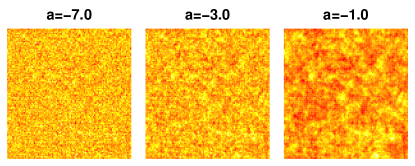
Figure 1: (color online) Slices of the same correlated disorder of a $97^{3}$ lattice for different correlation strengths. The random fields are heat coded. Bright means high positive field and dark means high negative field.

We tested our procedure by generating 20 realizations for $a=-1$ of the correlated disorder, calculating the two-point correlation Eq. (2) directly, and fitting Eq. (3) with variable exponent $a$. The correlation, shown in Fig. 2, and the resulting value $a=1.003(2)$ show that except for very small correlation at large distance the procedure works very well.

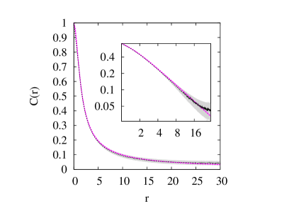
Figure 2: (color online) Mean of the two-point correlations for 20 arbitrary samples of long-range correlated random fields for $L=49,a=-1$ (black line) and error (gray background). The dashed (magenta) line is a fit according to Eq. (3) with $a=1.003(2)$ . The inset shows the same data as log-log-plot.

Next, we mention shortly how the exact ground states are calculated. The phase space of the uncorrelated RFIM consists of a ferromagnetic and a paramagnetic phase, see Fig. 3. The transition from one phase to the other can be triggered by varying the disorder strength $h$ or the temperature $T$. Changing both along a path $f(h,T)$ in the phase space leads to a critical point $P_{c}=(h_{c},T_{c})_{f(h,T)}$. From renormalization group calculations, the RFIM is known Bray and Moore (1985) to exhibit the same critical behavior at any $P_{c}$, except the temperature-driven phase transition point of the standard non-random Ising model. Hence, it is possible to focus on $T=0=\text{const.}$ and vary just $h$, to study the critical behavior along the full transition line. We do not know a-priori, whether the phase diagram for the correlated-disorder case has the same property, nevertheless, it makes sense to concentrate, at least for our study presented here, also on $T=0$.

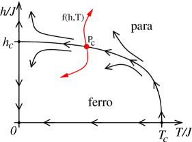
Figure 3: (color online) Schematic diagram of the phase space of the RFIM. The path $f(h,T)$ (red line) shows an arbitrary path to cross the phase boundary. The small arrows denote the renormalization group flow.

From the computational point of view this is very favorable, since it is possible to calculate exact ground states at $T=0$ in a very efficient way for system sizes as large as $N=141^{3}$ spins. Within this approach Picard and Ratliff (1975); Ogielski (1986), each realization of the correlated net fields $(\{\eta_{i}\},H)$ has to be mapped to a graph with $N+2$ nodes and $2N+1$ edges with suitable edge capacities. On this graph a sophisticated maximum flow/minimum cut algorithm can be applied.Goldberg and Tarjan (1988); Hartmann and Rieger (2001) The resulting minimum cut directly correspond to the GS spin configuration $\{S_{i}\}$ of that specific realization of the net disorder. We used the efficient maximum-flow subroutines implemented in the LEDA library.Mehlhorn and Näher (1999)

III Quantities of interest

From a GS spin configuration, some quantities of interest can be obtained directly, as the magnetization per spin

$$M=\frac{1}{N}\sum_{i}^{N}S_{i}\;$$ (10)

and the bond energy per spin

$$E_{J}=\frac{J}{N}\sum_{\langle i,j\rangle}S_{i}S_{j}\;,$$ (11)

Using these individual values, we calculate averaged quantities like the average magnetization $m=\langle M\rangle$. This disorder average $\langle\ldots\rangle$ is performed always for a fixed value of $h$. We also consider the Binder cumulant Binder (1981)

$$g(h,L)=\frac{1}{2}\left(3-\frac{\left\langle M^{4}\right\rangle}{\left\langle M^{2}\right\rangle^{2}_{h}}\right).$$ (12)

A specific-heat-like quantity $C(h)$ can be calculated as the numerical derivative of $E_{J}$ with respect to $h$ (see Ref. Hartmann and Young, 2001 for details). From here on we will refer to it as specific heat.

$$C(h)=\frac{\left\langle\partial E_{J}(h)\right\rangle}{\partial h}\;.$$ (13)

We also calculated the zero-temperature susceptibility

$$\chi(h)=\left.\frac{\partial m(h,H)}{\partial H}\right|_{H=0}\;$$ (14)

as linear response of the magnetization to small homogeneous magnetic fields $H$. Therefore, we apply small homogeneous fields at equidistant values $H_{1},2H_{1},3H_{1}$ and fit parabolas as function of $H$ to the magnetizations $m(h,H=0)$, $m(h,H_{1})$, $m(h,2H_{1})$ and $m(h,3H_{1})$. For a fixed value of the disorder strength $h$ the linear coefficient corresponds to the susceptibility $\chi(h)$.

We will see that the results are compatible with second order phase transitions, such that the measured quantities show power-law behavior close to the phase transition point. To determine the critical exponents, we use the standard scaling forms, i.e.,

$$g(h,L) = \tilde{g}\left((h-h_{c})L^{1/\nu}\right)\,,$$ (15)

$$m(h,L) =L^{-\beta/\nu} \tilde{m}\left((h-h_{c})L^{1/\nu}\right)\,,$$ (16)

$$\chi(h,L) =L^{\gamma/\nu} \tilde{\chi}\left((h-h_{c})L^{1/\nu}\right)\,,$$ (17)

$$C(h,L) =L^{\alpha/\nu} \tilde{C}\left((h-h_{c})L^{1/\nu}\right)\,,$$ (18)

and apply a finite-size scaling analysis. For the Binder cumulant and the magnetization we use a nice tool which performs data collapses automatically.Melchert (2009) It is based on a simplex algorithm and is written in python.

The specific heat and the susceptibility show a maximum close to the critical point. at some argument $f$ of the universal functions $\tilde{\chi}(\cdot)$ and $\tilde{C}(\cdot)$. Note that the peak positions for specific heat and susceptibility of the same system sizes $L$ usually differ. Thus, also the value of $f$ (and even the sign) may differ. From Eqs. (17) and (18) it follows that the finite-size dependence of the positions of the maxima, respectively, scale as

$$h^{*}(L)=h_{c}+f\cdot L^{-1/\nu}.$$ (19)

Furthermore, right at $h^{*}(L)$, the height of the maxima should scale as $L^{\gamma/\nu}$ and $L^{\alpha/\nu}$. In the case of $\alpha=0$ other forms like a logarithmic divergence or a convergence to a constant (“cusp”) have been observed for other systems in the literature.Yeomans (1993); Hartmann and Young (2001) Below we present the results we obtained for the position and the height of the peaks and test their scaling behaviour according to these scaling assumptions.

As mentioned above, these quantities are average values. They are strongly dependent on the set of disorder realizations taken into account. Hence, we perform an average usually over many thousands of realizations. We estimate the variability of these average values from $200$ bootstrap samples Efron et al. (1993); Hartmann (2009) and quote this as error.

IV Results

We performed exact ground-state calculations for three-dimensional RFIMs for correlation strengths $a=\{-1,-2,-3,-7\}$. We considered system sizes ranging from $L=7$ to $L=141$. The number of disorder realizations per system size and correlation strength can be found in Tab. 1. The actual number of calculated ground states is four times larger, since $4$ different external fields are needed to obtain a susceptibility. The values of $H_{1}$ are stated in the very right column of Tab. 1.

$L$	$a=-1$	$a=-2$	$a=-3$	$a=-7$	$H_{1}$
$7$	$33$	$33$	$33$	$33$	$0.0075$
$11$	$33$	$33$	$33$	$33$	$0.0050$
$15$	$13$	$32$	$61$	$182$	$0.0030$
$21$		$29$	$14$	$155$	$0.0025$
$25$	$90$	$32$		$150$	$0.0015$
$35$	$44$	$10$	$45$	$14$	$0.0015$
$49$	$32$	$26$	$16$	$16$	$0.0010$
$69$	$16$	$24$	$9$	$15$	$0.0005$
$97$	$20$	$8$	$4.5$	$9.5$	$0.0004$
$117$	$3$	$1$	$1.2$	$1.8$	$0.0002$
$141$	$1$	$0.2$	$0.2$	$0.3$	$0.0001$

Table 1: Number of disorder realizations per system size and correlation strength in thousands ($10^{3}$) and the external field $H_{1}$, used to calculate the susceptibility.

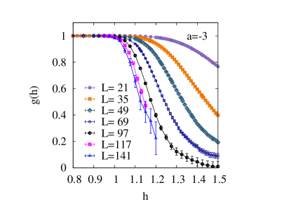
Figure 4: (color online) The Binder cumulant for $a=-3$ and different system sizes.

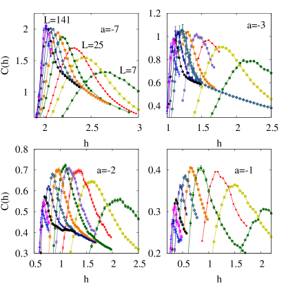
Figure 5: (color online) Specific-heat-like quantity for different correlation strengths $a=-7\dots a=-1$ and system sizes $L=7,11,15,21,25,35,49,69,97,117$ and $141$. For all values of $a$ the curves appear in monotonic ordering, meaning the curve of $L=7$ is on the very right and $L=141$ is on the very left, as labeled on the upper left subplot. The lines are guides to the eyes only.

Since the Binder cumulant exhibits no clear crossing (see Fig. 4) one could suspect that no phase transition is present. This is not the case as well will see in the following. To determine the phase transition points, we start by considering the average specific heat. In Fig. 5 the results can be seen for $a=-7$ to $a=-1$. As for the uncorrelated RFIM, peaks can be observed clearly, which give evidence for the existence of a phase transition also for the correlated case. We estimate the peaks by fitting parabolas over different intervals close to the maximum (for every bootstrap sample). The positions of the peaks in Fig. 5 move from right to left for increasing system sizes. To obtain the infinite-size limiting value $h_{c}$ and an estimate for the critical exponent $\nu$ of the correlation length, we fit the positions of the peaks to Eq. (19), resulting in fit values as shown in the upper part of Tab. 2. Note that when determining the error bars from model fitting, we usually have not only taken the statistical error obtained from the fit routine (of the gnuplot program) but we have always also varied the range of sizes, to get an impression of possible systematic errors.

In Fig. 5 for the case $a=-1$, the peaks move very close to $h=0$ and the result from the fit for $h_{c}$ is also close to zero. Therefore, another sensible ansatz is to set $h_{c}=0$. Fit parameters for this ansatz are also shown in Tab. 2 in the lower part. Both models are plotted in Fig. 6 as solid or broken lines, respectively. For $a<-1$, clearly $h_{c}>0$ is better compatible with the data points, while for $a=-1$ no real decision can be made here between $h_{c}>0$ and $h_{c}=0$. Nevertheless, $h_{c}(L)$ also looks slightly curved in the double-logarithmic plot, hence $h_{c}>0$ appears more likely here as well.

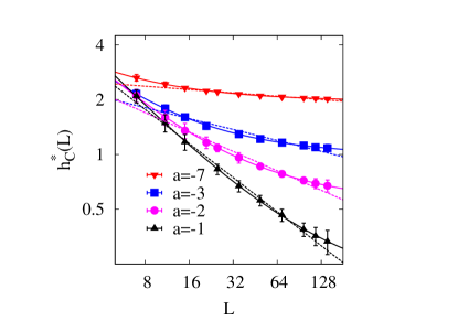
Figure 6: (color online) Peak positions of the specific-heat-like quantity as function of the system sizes for $a=-7\dots a=-1$. The solid lines are fits assuming a finite critical value according to Eq. 19, the broken ones are fits imply $h_{c}=0$.

	$a=-7$	$a=-3$	$a=-2$	$a=-1$
$h_{c}$	$1.962(4)$	$0.992(8)$	$0.537(8)$	$0.183(9)$
$f$	$3.2(1)$	$6.0(3)$	$7.5(2)$	$9.8(3)$
$1/\nu$	$0.79(2)$	$0.84(2)$	$0.81(2)$	$0.84(2)$
assuming no critical point $\Leftrightarrow h_{c}=0$
$f_{0}$	$2.62(5)$	$2.61(8)$	$3.1(1)$	$5.5(3)$
$1/\nu_{0}$	$0.055(5)$	$0.187(8)$	$0.32(1)$	$0.58(1)$

Table 2: Fit parameters of Eq. 19 for the peak position of the specific-heat-like quantity. The upper part contains the parameters for finite $h_{c}$. For the lower part $h_{c}=0$ was fixed.

To determine the critical exponent $\alpha$ according to Eq. (18), we analyzed the peak heights of the specific heat as shown in Fig. 7. They increase up to $L\approx 50$ for all correlation strengths $a$ and decrease for larger $L$. Thus, no clear scaling is visible. This could be due to very strong finite-size corrections. Therefore, under the assumption that the specific heat decreases in a power-law fashion, we fitted the data points for very large system sizes a power law of the form

$$C(h,L) =kL^{\alpha/\nu}\,.$$ (20)

The achieved exponents are small and negative can be found in Tab. 3.On the other hand it may be that the specific heat levels off for even larger system sizes, which would give the leading behavior $\alpha=0$. In Sec. VI, we will discuss these two options in connection with the Rushbrooke inequality Rushbrooke (1963) and see that $\alpha=0$ appears to be more likely.

	$a=-7$	$a=-3$	$a=-2$	$a=-1$
$k$	$2.3(2)$	$1.7(1)$	$1.9(1)$	$1.0(1)$
$\alpha/\nu$	$-0.04(2)$	$-0.11(2)$	$-0.26(1)$	$-0.24(3)$

Table 3: Fit parameters of Eq. 20 of the height of the maxima of the specific-heat as shown in Fig. 7

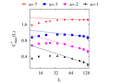
Figure 7: (color online) Peak heights of the specific heat as function of the system sizes for $a=-7\dots a=-1$. The lines are fits assuming a power law decay for large system sizes.

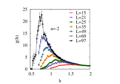
Figure 8: (color online) Susceptibility for $a=-2$.

We now turn to the susceptibility. The phase transition is signaled by a divergence of the susceptibility. An increasing peak can be seen for $a=-2$ in Fig. 8 as example. The peaks are estimated in the same way as for the specific heat. The resulting maxima are tuples $\left(h^{*}(L),\chi_{max}(L)\right)$ of position and height.

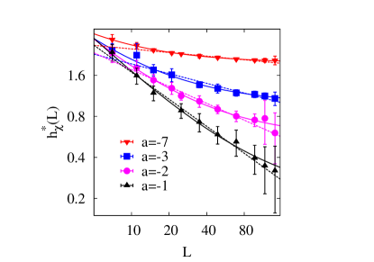
Figure 9: (color online) Peak positions of the susceptibility as function of the system sizes for $a=-7\dots a=-1$. The solid lines are fits assuming a finite critical value according to Eq. 19, the broken ones are fits imply $h_{c}=0$. .

For the peak position of the susceptibility we assumed the same model as we did for the specific heat. The models and data points can be found in Fig. 9.In particular for $a=-1$, the error bars are quite large, despite the large number of samples, which is for the largest system sizes considerably higher compared to the cases $a<-1$. To understand this behavior we studied the degree of non-self averaging Wiseman and Domany (1998) and we calculated

$$R_{\chi}\!(L)=\text{var}(\chi(L))/\langle\chi(L)\rangle^{2}.$$ (21)

We found $R_{\chi}$ to stay approximately constant for increasing $L$, as shown in Fig. 10 for susceptibility measured at the peak positions. We found the same behavior qualitatively for different fixed values of $h$, which shows that the correlated RFIM is non-self averaging for a large range of the disorder parameter, as many other systems exhibiting quenched disorder. In particular, the results in Fig. 10 show that the degree of non-self averaging is strongest for $a=-1$, which explains the large error bars. To achieve much smaller error bars for the susceptibility, a much larger number of samples would be necessary, which is beyond the capacity of our numerical resources.

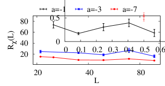
Figure 10: (color online) Ratio $R_{\chi}\!(L)$ for $a=-7,-3-1$. The data points for $a=-2$ lie between $a=-7$ and $a=-3$ and are not included for better visibility.

For the finite-size scaling of the peak-positions, we tested Eq. (19) using the saturating ansatz ($h_{c}$ included in the fit) as well as a pure power law decay (via $h_{c}\equiv 0$). The fit parameters for both models can be found in Tab. 4. Again the saturating model brings up, within the present accuracy, the same infinite-size critical point $h_{c}$ as we found before. Due to the error bars, we can not rule out a $h_{c}=0$ for $a=-1$, while for $a<-1$ again clearly $h_{c}>0$ holds.

	$a=-7$	$a=-3$	$a=-2$	$a=-1$
$h_{c}$	$1.97(1)$	$0.98(4)$	$0.56(4)$	$0.20(5)$
$f$	$4.8(5)$	$7(1)$	$9(1)$	$11(2)$
$1/\nu$	$0.83(5)$	$0.84(8)$	$0.85(7)$	$0.88(8)$
assuming no critical point $\Leftrightarrow h_{c}=0$
$f_{0}$	$3.06(8)$	$3.4(3)$	$4.5(4)$	$7.7(7)$
$1/\nu_{0}$	$0.088(7)$	$0.24(2)$	$0.41(3)$	$0.66(3)$

Table 4: Fit parameters of Eq. 19 of the peak position of the susceptibility. The upper part contains the parameters for finite $h_{c}$. For the lower part $h_{c}=0$ was fixed.

	$a=-7$	$a=-3$	$a=-2$	$a=-1$
$b_{0}$	$0.064(3)$	$0.049(2)$	$0.049(2)$	$0.041(3)$
$\gamma/\nu$	$1.56(1)$	$1.45(1)$	$1.34(2)$	$1.20(2)$

Table 5: Fit parameters of the peak heights of the susceptibility when fitting according to $b_{0}L^{\gamma/\nu}$.

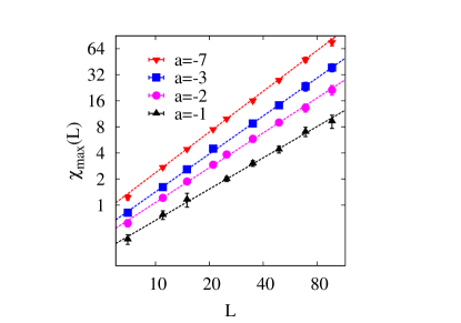
Figure 11: (color online) Peak heights of the susceptibility as function of the system sizes for $a=-3\dots a=-1$.

In contrast to the specific heat, the peak heights of the susceptibility shows a clear power law behaviour for all studied correlation strengths, see Fig. 11. Thus, in the thermodynamic limit the susceptibility diverges. Compared to the peak positions displayed in Fig. 9, the fluctuations for the peak height are much smaller, thus a clear power-law behavior is visible. The critical exponents $\gamma/\nu$, as obtained from a power-law fit, are displayed in Tab. 5. The values decreases with increasing $a$.

For a finite-size analysis of the Binder cumulant and of the magnetization we performed data collapses according to Eqs. (15) and (16). Example data collapses for the magnetization and as inset for the Binder cumulant for $a=-3$ are shown in Fig. 12. One sees that the quality of the collapses is very good. These lead to sets of critical values and exponents as shown in Tab. 6.

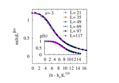
Figure 12: (color online) Data collapse of the magnetization and of the Binder cumulant (inset) for $a=-3$.

	$a=-7$	$a=-3$	$a=-2$	$a=-1$
$h_{c}$	$1.94(1)$	$0.95(2)$	$0.47(4)$	$0.12(3)$
$1/\nu$	$0.78(2)$	$0.77(4)$	$0.75(3)$	$0.78(4)$
$\beta/\nu$	$0.005(5)$	$0.03(2)$	$0.01(1)$	$0.01(8)$

Table 6: Critical value $h_{c}$ and correlations length exponent $\nu$ derived from the finite size scaling analysis of the Binder cumulant and the magnetization. These values are obtained via data collapses.

V Minimum and maximum correlated disorder

The minimum correlation range of the disorder is $a\rightarrow-\infty\equiv\delta$-correlated disorder, i.e. the normal RFIM. The other extreme is $a\to 0^{-}$. As it is illustrated in Fig. 1, by increasing the correlation strength $a$, the regions of sites with almost the same sign of the field get larger and larger, while keeping the same average close to 0. Hence, for $a\to 0^{-}$ one can imagine each realization of the disorder being bi-parted. Bi-parted means, to find two distinct clusters $\mathcal{A}=\{\eta_{i}>0\}$ and $\mathcal{B}=\{\eta_{i}<0\}$, see Fig. 13. An Imry-Ma type of argument would read as follows: In such a disorder realization, for a state where all spins are aligned with its local field, the resulting interface energy between the clusters $\mathcal{A,B}$ would be $E_{I}\sim L^{d_{f}}$ with fractal exponent $d-1\leq d_{f}\leq d$. This competes against the field energy $E_{h}\sim-hL^{d}$: If $E_{I}<|E_{h}|$, the ground-state will be an ordered phase, otherwise both clusters are locally aligned. A $T=0$ phase transition occurs when $|E_{h}|=E_{I}$. From this we see that the finite-size critical point scales in the limit $a\to 0^{-}$ as $h_{c}\sim L^{d_{f}-d}\to 0$ for $L\to\infty$. This means for highly correlated but arbitrarily small disorder the RFIM will behave as a super paramagnet in a field in the thermodynamic limit. Though, there would be no disorder-driven phase transition anymore. Furthermore, since the number of spins at distance $r$ scales as $r^{d-1}$ but the disorder correlation decreases only as $r^{a}$, its appears plausible that even for a finite range of $a<0$ values the cumulative effect of the correlation might dominate and indeed $h_{c}=0$ already for these values of $a$. This explains why the result for $a=-1$ is ambiguous.

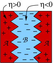
Figure 13: (color online) System with bi-parted random field (with periodic boundaries).

VI Conclusion and Discussion

We have presented the results of exact ground-state calculations of the RFIM with correlated disorder for different correlations strengths. To numerically calculate the ground states, we have applied a mapping to the maximum-flow problem. Using efficient polynomial-time-running maximum-flow/minimum-cut algorithms, we were able to study large systems sizes up to $N=141^{3}$.

We studied different quantities like magnetization, Binder cumulant, susceptibility and a specific heat-like quantity and applied finite-size scaling techniques to obtain the critical exponents. The combined results for the critical exponents are shown in Tab. 7. We tested the two possibilities for the values of $\alpha$, by applying the Rushbrooke inequality $\alpha+2\beta+\gamma\geq 2$ which holds usually as equality.Rushbrooke (1965) When choosing $\alpha=0$, the Rushbrooke equation is fulfilled in all cases within error bars. For the values of $\alpha$ quoted in Tab. 3, obtained via fitting the data for just the few largest systems sizes, the Rushbrooke sum is (assuming $h_{c}>0$) considerably smaller than 2 for $a=-2,-1$. Hence, the value $\alpha=0$ appears to be more likely. Note in all cases, the values quoted in the table are compatible within error bars with the results for the uncorrelated case, in particular due to the relative large error bar for the critical exponent $\gamma$. Nevertheless, the data for the peak heights of the susceptibility (Fig. 11) show a trend towards a smaller slope when increasing $a$ from $-7$ to $-1$: The results for $\gamma/\nu$, which are very precise (see Tab. 5) are clearly different within error bars. In this case, to still fulfill the Rushbrooke inequality, the true value for $\nu$, in particular for values $a=-2$ and $a=-1$, should be larger, at or somehow above the upper bounds given the standard error bars. Hence, it is quite likely that the correlation of the disorder creates non-universality for the RFIM, as in the case of the diluted ferromagnet.Ballesteros and Parisi (1999). Also, among our results, the case $a=-1$ is special. As discussed above, it appears plausible for $a=-1$ that the cumulative effect of the correlation might dominate. This would lead to $h_{c}=0$ already for $a=-1$. The result $h_{c}=0$ is indeed possible, as shown in last row of Tab. 7: Also on the base of the Rushbrooke sum, we cannot take decision on this issue. Nevertheless, numerically the inequality is much better fulfilled when assuming $h_{c}=0$.

$a$	$h_{c}$	$\alpha$	$\beta$	$\gamma$	$\nu$	RS sum
$-\infty$	$2.27(1)$	$\sim 0$	$0.016(7)$	$2.1(1)$	$1.37(9)$	$2.1(2)$
$-7$	$1.96(2)$	$0$	$0.01(1)$	$2.0(3)$	$1.26(8)$	$2.0(3)$
$-3$	$0.97(2)$	$0$	$0.04(6)$	$1.8(4)$	$1.2(2)$	$1.8(5)$
$-2$	$0.52(5)$	$0$	$0.01(3)$	$1.7(3)$	$1.2(2)$	$1.7(4)$
$-1$	$0.17(5)$	$0$	$0.05(10)$	$1.5(3)$	$1.2(2)$	$1.5(5)$
$-1^{*}$	$0$	$0$	$0.1(1)$	$1.9(1)$	$1.61(9)$	$2.0(4)$

Table 7: Final results for the value of $h_{c}$, the critical exponents $\alpha,\beta,\gamma$ and $\nu$ and the Rushbrooke (RS) sum $\alpha+2\beta+\gamma$. The first line shows the result for the uncorrelated case taken from Refs. Hartmann and Young, 2001; Middleton and Fisher, 2002. The last line is for the assumption $h_{c}(a=-1)=0$.

VII Acknowledgments

We would like to thank K. Janzen for fruitful discussions and critically reading the manuscript. Furthermore, we are grateful to M. Niemann helpful comments. The calculations were carried out on GOLEM (Großrechner OLdenburg für Explizit Multidisziplinäre Forschung) and the HERO (High-End Computing Resource Oldenburg) at the University of Oldenburg.

References

- Bricomont and Kupiainen (1987) J. Bricomont and A. Kupiainen, Phys. Rev. Lett. 59, 1829 (1987).
- Gofman et al. (1993) M. Gofman, J. Adler, A. Aharony, A. B. Harris, and M. Schwartz, Phys. Rev. Lett. 71, 1569 (1993).
- Rieger (1995) H. Rieger, Phys. Rev. B 52, 6659 (1995).
- Nowak et al. (1998) U. Nowak, K. D. Usadel, and J. Esser, Physica A: Statistical and Theoretical Physics 250, 1 (1998).
- Hartmann and Nowak (1999) A. K. Hartmann and U. Nowak, Eur. Phys. J. B 7, 105 (1999).
- Hartmann and Young (2001) A. K. Hartmann and A. P. Young, Phys. Rev. B 64, 214419 (2001).
- Middleton and Fisher (2002) A. A. Middleton and D. S. Fisher, Phys. Rev. B 65, 134411 (2002).
- Frontera and Vives (2002) C. Frontera and E. Vives, Computer Physics Communications 147, 455 (2002).
- Seppälä et al. (2002) E. T. Seppälä, A. M. Pulkkinen, and M. J. Alava, Phys. Rev. B 66, 144403 (2002).
- Hartmann (2002) A. K. Hartmann, Phys. Rev. B 65, 174427 (2002).
- Middleton (2002) A. A. Middleton, preprint arXiv:cond-mat/0208182 (2002).
- Zumsande et al. (2008) M. Zumsande, M. J. Alava, and A. K. Hartmann, J. Stat. Mech. p. P02012 (2008).
- Ahrens and Hartmann (2011) B. Ahrens and A. K. Hartmann, Phys. Rev. B 83, 014205 (2011).
- Fedorenko and Kühnel (2007) A. A. Fedorenko and F. Kühnel, Phys. Rev. B 75, 174206 (2007).
- Makse et al. (1996) H. A. Makse, S. Havlin, M. Schwartz, and H. E. Stanley, Phys. Rev. E 53, 5445 (1996).
- Ballesteros and Parisi (1999) H. G. Ballesteros and G. Parisi, Phys. Rev. B 60, 12912 (1999).
- Hod and Keshet (2004) S. Hod and U. Keshet, Phys. Rev. E 70, 015104 (2004).
- Fedorenko (2008) A. A. Fedorenko, Phys. Rev. B 77, 094203 (2008).
- Weinrib and Halperin (1983) A. Weinrib and B. I. Halperin, Phys. Rev. B 27, 413 (1983).
- Harris (1974) A. B. Harris, Journal of Physics C: Solid State Physics 7, 1671 (1974), URL http://stacks.iop.org/0022-3719/7/i=9/a=009.
- Ballesteros et al. (1999) H. G. Ballesteros, L. A. Fernández, V. Martín-Mayor, A. M. Sudupe, G. Parisi, and J. J. Ruiz-Lorenzo, Journal of Physics A: Mathematical and General 32, 1 (1999), URL http://stacks.iop.org/0305-4470/32/i=1/a=004.
- Ballesteros et al. (1998) H. G. Ballesteros, L. A. Fernández, V. Martín-Mayor, A. Muñoz Sudupe, G. Parisi, and J. J. Ruiz-Lorenzo, Phys. Rev. B 58, 2740 (1998).
- (23) Papercore is a free and open access database for summaries of scientific (currently mainly physics) papers., URL http://www.papercore.org/.
- Peng et al. (1991) C.-K. Peng, S. Havlin, M. Schwartz, and H. E. Stanley, Phys. Rev. A 44, R2239 (1991).
- Prakash et al. (1992) S. Prakash, S. Havlin, M. Schwartz, and H. E. Stanley, Phys. Rev. A 46, R1724 (1992).
- Frigo and Johnson (2005) M. Frigo and S. G. Johnson, Proceedings of the IEEE 93, 216 (2005), special issue on “Program Generation, Optimization, and Platform Adaptation”.
- Bray and Moore (1985) A. J. Bray and M. A. Moore, J. Phys. C: Solid State Phys. 18, 927 (1985).
- Picard and Ratliff (1975) J. C. Picard and H. D. Ratliff, Networks 5, 357 (1975).
- Ogielski (1986) A. T. Ogielski, Phys. Rev. Lett. 57, 1251 (1986).
- Goldberg and Tarjan (1988) A. V. Goldberg and R. E. Tarjan, J. ACM 35, 921 (1988), ISSN 0004-5411.
- Hartmann and Rieger (2001) A. K. Hartmann and H. Rieger, Optimization Algorithms in Physics (Wiley-VCH, Berlin, 2001), ISBN 978-3-527-40307-3.
- Mehlhorn and Näher (1999) K. Mehlhorn and S. Näher, The LEDA Platform of Combinatorial and Geometric Computing (Cambridge University Press, Cambridge, 1999), URL http://www.algorithmic-solutions.de.
- Binder (1981) K. Binder, Z. Phys 43, 119 (1981).
- Melchert (2009) O. Melchert, Preprint: arXiv:0910.5403v1 (2009).
- Yeomans (1993) J. M. Yeomans, Statistical Mechanics of Phase Transitions (Oxford University Press, Oxford, 1993).
- Efron et al. (1993) B. Efron, B. Efron, and R. J. Tibshirani, An Introduction to the Bootstrap (Chapman & HALL/CRC, 1993).
- Hartmann (2009) A. K. Hartmann, A Practical Guide To Computer Simulation (World Scientific Publishing Company, 2009), ISBN 978-9812834157.
- Rushbrooke (1963) G. S. Rushbrooke, J. of Chem. Phys. 39, 842 (1963).
- Wiseman and Domany (1998) S. Wiseman and E. Domany, Phys. Rev. Lett. 81, 22 (1998).
- Rushbrooke (1965) G. S. Rushbrooke, J. of Chem. Phys. 43, 3439 (1965).