Synchronization in interdependent networks

Abstract

We explore the synchronization behavior in interdependent systems, where the one-dimensional (1D) network (the intranetwork coupling strength $J_{\rm I}$) is ferromagnetically intercoupled (the strength $J$) to the Watts-Strogatz (WS) small-world network (the intranetwork coupling strength $J_{\rm II}$). In the absence of the internetwork coupling ($J=0$), the former network is well known not to exhibit the synchronized phase at any finite coupling strength, whereas the latter displays the mean-field transition. Through an analytic approach based on the mean-field approximation, it is found that for the weakly coupled 1D network ($J_{\rm I}\ll 1$) the increase of $J$ suppresses synchrony, because the nonsynchronized 1D network becomes a heavier burden for the synchronization process of the WS network. As the coupling in the 1D network becomes stronger, it is revealed by the renormalization group (RG) argument that the synchronization is enhanced as $J_{\rm I}$ is increased, implying that the more enhanced partial synchronization in the 1D network makes the burden lighter. Extensive numerical simulations confirm these expected behaviors, while exhibiting a reentrant behavior in the intermediate range of $J_{\rm I}$. The nonmonotonic change of the critical value of $J_{\rm II}$ is also compared with the result from the numerical RG calculation.

Synchronization phenomenon is the one of the most fascinating collective emergent behaviors abundantly found in natural and artificial systems. The onset of synchronization occurs when the differences of individual oscillators are overcome by the strong coupling among elements. We investigate the coupled system of two networks, one is synchronizable at finite coupling strength while the other is not, aiming to answer the question of what happens as the inter- and intra-couplings are varied. For the weak intracouplings of the nonsynchronizable network, both our analytic and numerical results show that the stronger internetwork coupling hinders the synchronization in the synchronizable network since the nonsynchronized oscillators in the other network work as heavier burdens for the oscillators in the synchronizable network to carry to synchronize. On the other hand, as the intracoupling strength in the nonsynchronizable network becomes larger, partially synchronized groups of more oscillators are formed, which in turn help the oscillators in the synchronizable network to become unified as synchronized clusters. In the intermediate regime where the intra- and inter-network couplings are in the same order of magnitude, numerical results show a reentrant behavior in the synchronization phase diagram.

I Introduction

Synchronization as a collectively emergent phenomenon in complex systems has attracted much interest thanks to the abundance of examples in nature intro1 ; intro2 ; intro3 ; Kuramoto . In existing studies, it has been revealed that the topology of interaction plays an important role in synchronizability synch ; synchER . In particular, it is now well known that coupled phase oscillators described by the celebrated Kuramoto model Kuramoto exhibit various universality classes depending on dimensionality and the topological structure of networks synchER ; synchWS ; ott ; synchSF ; lattice1 ; lattice2 . It has also been found that the lower critical dimension for the frequency synchronization in the regular $d$-dimensional Kuramoto model is $d=2$, while the corresponding lower critical dimension for the phase synchronization transition with the spontaneous $O(2)$ symmetry breaking is $d=4$ lattice1 ; lattice2 . Moreover, numerical studies lattice2 have implied that systems of $d>4$ belong to the mean-field (MF) universality class as shown in globally coupled oscillators. On the other hand, for the Kuramoto model in complex networks, various results have been reported: For random and small-world networks ER ; WS , it has been observed that the MF transition exists synchER ; synchWS , and for scale-free (SF) network with a power-law degree distribution $\rho\sim k^{-\gamma}$, where $k$ stands for degree, $\gamma$-dependent critical exponents have been found via a MF approximation and numerical investigations synchSF .

In the present work, we couple the one-dimensional (1D) network and the Watts-Strogatz (WS) small-world network WS (see Fig. 1), and investigate the synchronizability of Kuramoto oscillators in the composite two coupled networks. Our research focus is put on the effect of internetwork coupling between the two networks belonging to different universalities, i.e., the MF universality for the WS network and the absence of the synchronous phase for the 1D regular network. The physics of coupled interdependent networks are not only interesting in the pure theoretical point of view, but it also can have practical applicability since these interdependent network structures can be found ubiquitously. For example, electric power distribution in the power grid is strongly interwoven with the communication through Internet, and thus spreading of failures in one network affects failures in other network inter1 ; inter2 . This coupled system has been studied within the framework of percolation with the strength of internetwork coupling varied; strong coupling between networks yields a first-order transition, while in weakly coupled networks a giant cluster continuously vanishes at the critical point inter3 . In Ref. jo, , the epidemic spreading behavior has been studied in the coupled networks of the infection layer and the prevention layer. We believe that the study of the collective synchronization in interdependent networks can also be an important realistic problem in a broader context: Imagine that each agent in a social system has two different types of dynamic variables and that the interaction of the one type of variable has different interaction topology than the other variable. We emphasize that our study of the synchronization in coupled networks is worthwhile because it could be applicable to investigate social collective behaviors in interdependent networks. Another interesting example of the interdependent system can be found in the neural network in the brain: The cortical region is coupled with the thalamus inter4 , and the thalamocortical interactions might be interpreted as the intercoupling between the cortical area and thalamus.

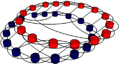
Figure 1: (Color online) Two coupled interdependent networks: The one-dimensional regular network (the upper one) with the periodic boundary condition is coupled to the Watts-Strogatz small-world network (the lower one). Both networks have the average degrees four.

II Model

We consider the composite system of two coupled networks (I and II) with equal number $N$ of oscillators for each. The equations of motion for the Kuramoto model in the system are given by

$$\dot{\phi}^{\rm I}_{j}=\omega^{\rm I}_{j}-J\sin(\phi^{\rm I}_{j}-\phi^{\rm II}_{j})-J_{\rm I}\sum_{l}^{N}a^{\rm I}_{jl}\sin(\phi^{\rm I}_{j}-\phi^{\rm I}_{l}),\;\;\dot{\phi}^{\rm II}_{j}=\omega^{\rm II}_{j}-J\sin(\phi^{\rm II}_{j}-\phi^{\rm I}_{j})-J_{\rm II}\sum_{l}^{N}a^{\rm II}_{jl}\sin(\phi^{\rm II}_{j}-\phi^{\rm II}_{l}),$$ (1)

where $\phi^{\rm I(II)}_{j}$ is the phase of the $j$th oscillator and $\omega^{\rm I(II)}_{j}$ is its intrinsic frequency in the network I (II), assumed as an independent quenched random Gaussian variable with the unit variance. Throughout the paper, we denote the 1D regular network as the network I and the WS network as II, and use the average degree $\langle k\rangle=4$ for both. The adjacency matrix for the 1D network has elements $a^{\rm I}_{jl}=\delta_{j,l\pm 1}+\delta_{j,l\pm,2}$, while $a^{\rm II}_{jl}$ is constructed following the small-world network generation method: Each link is visited and rewired at the probability $p$ (see Ref. WS for details). In Eq. (1), $J$ denotes the internetwork coupling strength between I and II, and $J_{\rm I(II)}$ stands for the intranetwork coupling for the network I(II). One may expect that when $J$ becomes large enough the partial synchronization in the 1D regular network could be induced by the established ordering in the WS network although no spontaneous ordering exists in the pure 1D network. On the other hand, if $J_{\rm I}$ is not big enough, the internetwork coupling $J$ to the nonsynchronized 1D network could also make the WS network itself hard to synchronize. It is also possible that if $J_{\rm I}$ is infinite, yielding fully synchronized 1D oscillators, synchronization is induced in the WS network even at $J_{\rm II}=0$. The interplay among these inter- and intra-network couplings can provide rich phenomena, the understanding of which composes the main motivation of the present study.

III Analytic Results

III.1 Mean-field analysis for $J=0$

When the two networks are decoupled, i.e., when $J=0$ in Eq. (1), the network II should show the MF synchronization transition as reported in previous studies synchWS . In this Section, we briefly review the MF theory of the Kuramoto model for the single WS network ott ; synchSF . The equations of motion for the network II without $J$ is rewritten as

$$\dot{\phi}^{\rm II}_{j}=\omega^{\rm II}_{j}-J_{\rm II}k^{\rm II}_{j}H_{j}\sin(\phi^{\rm II}_{j}-\theta_{j}),$$ (2)

where we have used $H_{j}e^{i\theta_{j}}\equiv(1/k^{\rm II}_{j})\sum_{l}^{N}a^{\rm II}_{jl}e^{i\phi^{\rm II}_{l}}$ with $k^{\rm II}_{j}$ being the degree of the $j$th node in II. In the spirit of the MF approximation, we neglect the fluctuation and substitute $H_{j}$ and $\theta_{j}$ by global variables $H$ and $\theta$, respectively, which yields the self-consistent equation for the order parameter $H$:

$$H=\frac{1}{N\langle k_{\rm II}\rangle}\sum^{N}_{j}k^{\rm II}_{j}\sqrt{1-\left(\frac{\omega^{\rm II}_{j}}{k^{\rm II}_{j}HJ_{\rm II}}\right)^{2}}\Theta\left(1-\frac{|\omega^{\rm II}_{j}|}{k^{\rm II}_{j}HJ_{\rm II}}\right),$$ (3)

where $\Theta(x)$ is the Heaviside step function [$\Theta(x)=1(0)$ for $x\geq 0$ ($<0$)]. In thermodynamic limit of $N\to\infty$, we change the sum over oscillators to the sum over different degrees, which gives us

$$H=\frac{1}{\langle k_{\rm II}\rangle}\sum_{k_{\rm II}}\rho(k_{\rm II})k_{\rm II}u(k_{\rm II}HJ_{\rm II}),$$ (4)

where $\rho(k_{\rm II})$ is the degree distribution function and

$$u(x)\equiv\int^{x}_{-x}d\omega_{\rm II}g(\omega_{\rm II})\sqrt{1-\omega_{\rm II}^{2}/x^{2}}$$ (5)

with $g(\omega_{\rm II})=\exp(-\omega_{\rm II}^{2}/2\sigma_{\rm II}^{2})/\sqrt{2\pi}\sigma_{\rm II}$. Note that near the critical point where $H$ becomes vanishingly small, Eq. (5) is expanded in the form $u\approx\frac{\pi}{2}g(0)k_{\rm II}HJ_{\rm II}+\frac{\pi}{16}g^{\prime\prime}(0)[k_{\rm II}HJ_{\rm II}]^{3}$, which leads to

$$H=\frac{\langle k^{2}_{\rm II}\rangle\pi}{2\langle k_{\rm II}\rangle}g(0)J_{\rm II}H+\frac{\langle k^{4}_{\rm II}\rangle\pi}{16\langle k_{\rm II}\rangle}g^{\prime\prime}(0)J^{3}_{\rm II}H^{3}.$$ (6)

Here, it is to be noted that since the network II is the WS network with the exponential degree distribution, both $\langle k^{2}_{\rm II}\rangle$ and $\langle k^{4}_{\rm II}\rangle$ have well-defined finite values. It is then straightforward to get the critical point $J^{\rm II}_{c}=\frac{2\langle k_{\rm II}\rangle\sigma_{\rm II}\sqrt{2}}{\langle k^{2}_{\rm II}\rangle\sqrt{\pi}}$ and the critical exponent $\beta=1/2$. Moreover, introducing a sample-to-sample fluctuation synchSF to the right-hand side of Eq. (6), we obtain the finite-size scaling (FSS) exponent $\bar{\nu}=5/2$.

III.2 Mean-field analysis for $J_{\rm I}\ll 1$

We next turn our attention to the coupled system ($J\neq 0$), and first consider the case of vanishingly small intranetwork coupling for I. As $J_{\rm I}\to 0$, dynamics in the network I is simply governed by $\dot{\phi_{\rm I}}=\omega_{\rm I}-J\sin(\phi_{\rm I}-\phi_{\rm II})$ with the site index omitted for convenience. For $\langle\omega_{\rm I}\rangle=\langle\omega_{\rm II}\rangle=0$, running oscillators in I with $\dot{\phi_{\rm I}}\neq 0$ may hinder their connected counterpart oscillators in II from entering into the global entrainment. It has also been found that contributions of detrained oscillators to the synchronization order parameter are negligible within the MF theory ott ; synchSF . Accordingly, one can make the plausible assumption that entrained oscillators ($\dot{\phi_{\rm I}}=0$) in I and their corresponding oscillators in II mainly contribute to the synchronization. We then write the equations of motion for the entrained oscillators in II as

$$\dot{\phi}_{\rm II}=\omega_{\rm II}+\tilde{\omega}_{\rm I}-J_{\rm II}k_{\rm II}H\sin(\phi_{\rm II}-\theta),$$ (7)

where $\tilde{\omega}_{\rm I}\equiv J\sin(\phi_{\rm I}-\phi_{\rm II})$ with $|\tilde{\omega}_{\rm I}|\leq J$, and the MF approximation ($H_{j},\theta_{j})\rightarrow(H,\theta)$ has been made in the assumption that the internetwork coupling does not change the universality of II since there exists no ordering in I for $J_{\rm I}\rightarrow 0$. Consequently, the self-consistent equation reads $H=\left(N^{\prime}\langle k_{\rm II}\rangle\right)^{-1}\sum_{j}^{N^{\prime}}k^{\rm II}_{j}\sqrt{1-f_{j}^{2}}\Theta(1-|f_{j}|)$, where $f_{j}\equiv(\omega^{\rm II}_{j}+\tilde{\omega}^{\rm I}_{j})/k^{\rm II}_{j}HJ_{\rm II}$ and $N^{\prime}\equiv N\int_{-J}^{J}d\omega_{\rm I}g(\omega_{\rm I})$. In thermodynamic limit of $N\to\infty$, we again meet the form of $H=(1/\langle k_{\rm II}\rangle)\sum_{k_{\rm II}}\rho(k_{\rm II})k_{\rm II}u(x)$ with

$$u(x)\equiv\int_{-J}^{J}d\omega_{\rm I}\tilde{g}(\omega_{\rm I})\int^{x-\omega_{\rm I}}_{-x-\omega_{\rm I}}d\omega_{\rm II}g(\omega_{\rm II})\sqrt{1-\left(\frac{\omega_{\rm II}+\omega_{\rm I}}{x}\right)^{2}},$$ (8)

where $x=k_{\rm II}HJ_{\rm II}$ and $\tilde{g}(\omega_{\rm I})=\mathcal{N}^{-1}e^{-\omega^{2}_{\rm I}/2\sigma^{2}_{\rm I}}$ with the normalization constant $\mathcal{N}=\int_{-J}^{J}d\omega_{\rm I}e^{-\omega^{2}_{\rm I}/2\sigma^{2}_{\rm I}}$. Following the similar steps to those made for $J=0$, we conclude that the synchronization transition occurs at the critical value $J^{\rm II}_{c}=\frac{2\langle k_{\rm II}\rangle}{A\langle k^{2}_{\rm II}\rangle\pi}$ with a constant

$$A\equiv\left(\sqrt{2\pi\sigma^{2}_{\rm II}}\mathcal{N}\right)^{-1}\int_{-J}^{J}d\omega_{\rm I}\exp\left[-\omega^{2}_{\rm I}\left(\frac{2\sigma^{2}_{\rm I}\sigma^{2}_{\rm II}}{\sigma^{2}_{\rm I}+\sigma^{2}_{\rm II}}\right)^{-1}\right].$$ (9)

We note from the expression that as $J$ is increased, $J_{c}^{\rm II}$ also increases since $A$ is decreased due to the fact that $\frac{\sigma^{2}_{\rm I}\sigma^{2}_{\rm II}}{\sigma^{2}_{\rm I}+\sigma^{2}_{\rm II}}<\sigma^{2}_{\rm I}$. Since $\sigma_{\rm I}=\sigma_{\rm II}$, one obtains $J_{c}^{\rm II}(J)=\frac{4\langle k_{\rm II}\rangle\sigma_{\rm II}}{\langle k^{2}_{\rm II}\rangle\sqrt{\pi}}=\sqrt{2}J_{c}^{\rm II}(0)$ with $J\to\infty$. Furthermore, it is expected that as $J_{\rm I}$ is increased (but still $J_{\rm I}\ll 1$) $J^{\rm II}_{c}$ should decrease from the following reasoning: When $J_{\rm I}\ll 1$, effective equations for oscillators in I can be written as $\dot{\phi_{\rm I}}=\omega^{\prime}_{\rm I}-J\sin(\phi_{\rm I}-\phi_{\rm II})$. Here, $\omega^{\prime}_{\rm I}$ is a modified frequency whose variance $\sigma^{\prime}_{\rm I}$ becomes smaller than the bare value due to the attractive force activated by the existence of the intranetwork coupling. We then conclude that $\sigma^{\prime}_{\rm I}\equiv\sigma^{\prime}_{\rm I}(J_{\rm I})$ is a decreasing function of $J_{\rm I}$. Substituting $\sigma_{\rm I}$ by $\sigma^{\prime}_{\rm I}$ in Eq. (9), one notes that $r(J_{\rm I})\equiv\sigma^{2}_{\rm II}/(\sigma^{\prime 2}_{\rm I}+\sigma^{2}_{\rm II})$ increases with $J_{\rm I}$, and thus $A=\left(\sqrt{2\pi\sigma_{\rm II}^{2}}\mathcal{N}\right)^{-1}\int_{-J}^{J}d\omega_{\rm I}\exp\left[-\omega_{\rm I}^{2}/\left(2r\sigma^{\prime 2}_{\rm I}\right)\right]$ with $\mathcal{N}=\int_{-J}^{J}d\omega_{\rm I}\exp\left[-\omega_{\rm I}^{2}/\left(2\sigma^{\prime 2}_{\rm I}\right)\right]$ becomes an increasing function (i.e., $J^{\rm II}_{c}$ becomes a decreasing function) with respect to $J_{\rm I}$. In summary of this subsection, when the 1D network is within the weakly coupled regime (i.e., when $J_{\rm I}$ is sufficiently small), the synchronization of the WS network is enhanced (i.e., $J^{\rm II}_{c}$ in reduced), as $J_{\rm I}/J$ is increased. In words, the stronger internetwork coupling puts more burden for the WS network to achieve its synchrony, while the better synchrony in the 1D network helps the WS network to be better synchronized via the internetwork coupling.

III.3 Renormalization group approach for $J_{\rm I}>J$

For a strong coupling regime of the 1D regular network, our MF equations in Sec. III.2 for $J_{\rm I}\to 0$ need to be modified by employing the real-space renormalization-group (RG) formulation that has been developed in the 1D systems RG . In this RG approach applied for 1D regular networks, strong bonds form clusters of entrained oscillators, while fast moving oscillators are decimated, interrupting the development of a giant synchronized cluster. In our system, it is expected that the strong coupling in the 1D regular network should induce synchronized clusters not only in the 1D regular network, but also in the WS network coupled to it via the internetwork coupling.

For $J_{\rm I}>J$, oscillators in the network I are governed mainly by intranetwork coupling rather than by internetwork coupling, which allows us to apply the RG approach to the 1D network with respect to $\omega_{\rm I}$ and $J_{\rm I}$: For $|\omega_{\rm I}|>J_{\rm I}>J$, $\omega_{\rm I}$ becomes relevant, whereas for $J_{\rm I}>|\omega_{\rm I}|>J$ and $J_{\rm I}>J>|\omega_{\rm I}|$, $J_{\rm I}$ becomes relevant. Applying the RG approach, fast moving oscillators having $|\omega_{\rm I}|>J_{\rm I}$ are removed from the 1D regular network together with their bonds, yielding fragmentation in I (our numerical RG calculations are summarized in Sec. IV). On the other hand, since the remaining bonds are strong enough, oscillators left in a fragment form a synchronized cluster with the phase $\Phi^{\rm I}_{j}$ and the renormalized frequency $\Omega^{\rm I}_{j}=(1/m^{\rm I}_{j})\sum_{i\in S^{\rm I}_{j}}\omega^{\rm I}_{i}$, where $m^{\rm I}_{j}\equiv|S^{\rm I}_{j}|$ is a number of oscillators in the $j$th cluster $S^{\rm I}_{j}$.

The entrainment of oscillators into clusters in the network I tends to drive oscillators in network II to cluster themselves in the same corresponding clusters because of the ferromagnetic intercouplings. For simplicity, we assume that the same number $N_{c}$ of clusters are generated both in I and II. Within the framework of the MF approximation, equations of motion are written as

$$\dot{\Phi}^{\rm I}_{j}=\Omega^{\rm I}_{j}-J\sin(\Phi^{\rm I}_{j}-\Phi^{\rm II}_{j}),\;\;\dot{\Phi}^{\rm II}_{j}=\Omega^{\rm II}_{j}-J\sin(\Phi^{\rm II}_{j}-\Phi^{\rm I}_{j})-\langle k_{\rm II}\rangle J_{\rm II}H\sin(\Phi^{\rm II}_{j}-\theta),$$ (10)

where $\Omega^{\rm II}_{j}=(1/m^{\rm II}_{j})\sum_{i\in S^{\rm II}_{j}}\omega^{\rm II}_{i}$ with $m^{\rm II}_{j}$ being the number of oscillators in the $j$th cluster $S^{\rm II}_{j}$ in the network II. A set of oscillators $\{\phi^{\rm II}_{i}\}$ connected to $\Phi_{j}^{\rm I}$ are merged into $\Phi^{\rm II}_{j}$ except for ones with $|\omega_{\rm II}|>J$ since we only consider entrained clusters induced by the internetwork coupling. $\langle k_{\rm II}\rangle$ in Eq. (10) also arises from $(1/m^{\rm II}_{j})\sum_{i\in S^{\rm II}_{j}}k^{\rm II}_{i}\approx\langle k_{\rm II}\rangle$. Now, it is straightforward to obtain $J_{c}^{\rm II}$ from Eq. (10) via the same procedure as done for the case of $J_{\rm I}=0$, to yield

$$J^{\rm II}_{c}=\frac{2\sqrt{2\bar{\sigma}^{2}_{\rm I}+2\bar{\sigma}^{2}_{\rm II}}}{\langle k_{\rm II}\rangle\sqrt{\pi}},$$ (11)

where the approximation $\int_{-J}^{J}d\Omega_{\rm I}\approx\int_{-\infty}^{\infty}d\Omega_{\rm I}$ has been made from the assumption that $\bar{\sigma}_{\rm I}<J$. Here, $\bar{\sigma}^{2}_{\rm I(II)}$ is the variance for $\Omega_{\rm I(II)}$ within the Gaussian approximation, that is, $g(\Omega_{\rm I(II)})=e^{-\Omega^{2}_{\rm I(II)}/2\bar{\sigma}_{\rm I(II)}^{2}}/\sqrt{2\pi\bar{\sigma}^{2}_{\rm I(II)}}$. Note that $\bar{\sigma}_{\rm I}\sim\sigma_{\rm I}^{*}/\sqrt{\bar{m}_{\rm I}}$ and $\bar{\sigma}_{\rm II}\sim\sigma^{*}_{\rm II}/\sqrt{\bar{m}_{\rm II}}$, where $\bar{m}_{\rm I(II)}$ is the average number of oscillators forming a cluster in I(II), given by $\bar{m}_{\rm I(II)}=\left[N\int_{-J_{\rm I}(-J)}^{J_{\rm I}(J)}d\omega_{\rm I(II)}g(\omega_{\rm I(II)})\right]/N_{c}$, and $\sigma^{*}_{\rm I(II)}$ is obtained from $\sigma_{\rm I(II)}^{*2}=\int_{-J_{\rm I}(-J)}^{J_{\rm I}(J)}d\omega_{\rm I(II)}\omega^{2}_{\rm I(II)}\tilde{g}(\omega_{\rm I(II)})$ since the frequency of oscillators which consist of clusters in I(II) must be less than $J_{\rm I}$ ($J$). For sufficiently large $J$ and $J_{\rm I}$ yielding $\sigma^{*}_{\rm I(II)}\sim 1$ and $\bar{m}_{\rm I(II)}\sim N/N_{c}$, it is obtained that $J_{c}^{\rm II}\sim\sqrt{N_{c}/N}$, implying that the synchronization onset decreases with $J_{\rm I}$ since the number of clusters should be the decreasing function with large $J_{\rm I}$; only at $J_{\rm I}\to\infty$, $N_{c}/N$ becomes close to $1/N$, yielding $J_{c}^{\rm II}=0$ in thermodynamic limit.

We have above investigated the synchronization onset as a function of $J$ and $J_{\rm I}$ via the MF approximation. It has been found that for weakly coupled 1D oscillators, the internetwork coupling increases the synchronization onset, while increasing $J_{\rm I}$ enhances the synchronizability. The role of the strong intranetwork coupling in the 1D regular network has been revealed through the RG approach; clustering in the 1D network makes the synchronization easier.

For FSS exponent for $J_{\rm I}>0$, $\bar{\nu}=5/2$ still holds since the number of samples, i.e., $N^{\prime}$ or $N_{c}$ is proportional to the system size $N$ linearly: The density $N_{c}/N$ of clusters only depends on $J_{\rm I}$ since $\omega_{\rm I}$ is a random variable, yielding $N_{c}\sim N$.

IV Numerical results

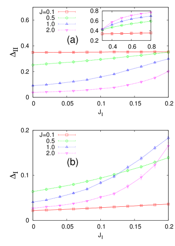
Figure 2: (Color online) Order parameters obtained through the numerical integrations of Eq. (1): (a) for the WS network ($\Delta_{\rm II}$) and (b) for the 1D regular network ($\Delta_{\rm I}$) versus the intranetwork coupling strength in the 1D network $J_{\rm I}$, at various values of internetwork coupling $J$ (the intranetwork coupling $J_{\rm II}$ in the WS network is set to 0.7 and the network size $N=12800$ for both I and II). For sufficiently small values of $J_{\rm I}$, the synchrony in II is suppressed (enhanced) as $J(J_{\rm I})$ is increased, as shown Sec. III.2 via the MF approach. Inset in (a): Further increase of $J_{\rm I}$ enhances the synchronization in II. The internetwork coupling $J$ plays a positive role for the synchronization in II, differently from the weak-coupling regime: As $J$ is increased at a fixed $J_{\rm I}$, $\Delta_{\rm II}$ is increased. (b) shows that for small values of $J_{\rm I}$ the increase of internetwork coupling first enhances synchrony in I and then reduces it as $J$ is increased further.

In order to validate our MF predictions, we perform numerical integrations of Eq. (1), with the network II constructed via the WS model WS at the rewiring rate $p=0.5$. After achieving the steady state, we measure the time-averaged order parameter

$$\Delta_{\rm I(II)}\equiv\frac{1}{T}\int_{T_{0}}^{T_{0}+T}dt\left<\frac{1}{N}\left|\sum_{j}^{N}e^{-i\phi_{j}^{\rm I(II)}\left(t\right)}\right|\right>,$$ (12)

where $\langle\dots\rangle$ stands for the average over different realizations of frequencies and networks.

First, we compute order parameters when the 1D network is in the weakly coupled regime (small $J_{\rm I}$) at fixed $J_{\rm II}$. In Fig. 2, we exhibit $\Delta_{\rm II}$ and $\Delta_{\rm I}$ as functions of $J_{\rm I}$ in (a) and (b), respectively. It is observed that as the internetwork coupling $J$ is increased, the order parameters $\Delta_{\rm I}$ and $\Delta_{\rm II}$ show a decreasing tendency, except for very small values of $J$ for $\Delta_{\rm I}$. The nonmonotonic change of $\Delta_{\rm I}$ with respect to $J$ is not surprising, since $\Delta_{\rm I}\approx 0$ as $J\rightarrow 0$ [see the curve for $J=0.1$ in Fig. 2(b)].

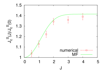
Figure 3: (Color online) Ratio $J_{c}^{\rm II}(J)/J_{c}^{\rm II}(0)$ as a function of $J$ at $J_{\rm I}=0$. Points are from the numerical integrations of Eq. (1) combined with the finite-size scalings in Eq. (13), while the line denotes the MF prediction made in Sec. III.2.

For $J_{\rm I}=0$, the synchronization onset $J_{c}^{\rm II}$ is evaluated using the FSS of the form

$$\Delta_{\rm II}=N^{-\beta/\bar{\nu}}f\bigl{(}(J_{\rm II}-J_{c}^{\rm II})N^{1/\bar{\nu}}\bigr{)}$$ (13)

with $\beta=1/2$ and $\bar{\nu}=5/2$, resulting in $J_{c}^{\rm II}(J)\approx$ 0.66, 0.68, 0.74, 0.8, 0.88, 0.89 and 0.91 at $J=$ 0, 0.5, 1.0, 1.5, 2.0, 3.0 and 4.0, respectively. In Fig. 3, it is observed that the ratio $J_{c}^{\rm II}(J)/J_{c}^{\rm II}(0)$ obtained numerically follows the MF prediction in Sec. III.2, given by $J_{c}^{\rm II}(J)/J_{c}^{\rm II}(0)=\int_{0}^{J}dxe^{-x^{2}/2}/\int_{0}^{J}dxe^{-x^{2}}$ with $\sigma_{\rm I}=\sigma_{\rm II}=1$. It is also found that $J_{c}^{\rm II}$ saturates at large $J$: $J_{c}^{\rm II}(4.0)/J_{c}^{\rm II}(0)\approx 1.4$, which is consistent with the MF value, $J_{c}^{\rm II}(J\to\infty)/J_{c}^{\rm II}(J=0)=\sqrt{2}$. Also in the weakly-coupled regime of small $J_{\rm I}(>0)$, it is again observed that $J_{c}^{\rm II}$ is increased as $J$ is increased, implying that the stronger internetwork coupling worsens the synchronizability of II, in agreement with the finding in Sec. III.2. Another MF prediction in Sec. III.2 that the increase of $J_{\rm I}$ enhances the synchrony in II is clearly confirmed in Fig. 2(a): At fixed $J$, the order parameter for II is an increasing function of $J_{\rm I}$. For larger $J_{\rm I}$, the $J$-dependence of $\Delta_{\rm II}$ shown in the inset for Fig. 2(a) can be interpreted as follows: More oscillators should be involved in synchronization with stronger internetwork coupling in I, and thus the order parameter increases as $J$ is increased, which may be implying that $J_{c}^{\rm II}$ is decreasing with $J$ at large $J_{\rm I}$ in contrast to the case for the weak coupling regime of small $J_{\rm I}$. Consequently, we conclude that the role of the internetwork coupling $J$ is reversed in the weak and the strong coupling regimes: For the weakly (strongly) coupled 1D network, internetwork coupling worsens (enhances) the synchrony in the WS network.

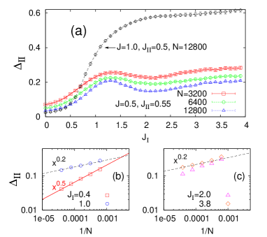
Figure 4: (Color online) (a) $\Delta_{\rm II}$ versus $J_{\rm I}$ at $J=0.5$ and $J_{\rm II}=0.55$ for various system sizes. Nonmonotonic change of $\Delta_{\rm II}$ is observed at all system sizes. $N$-dependence of $\Delta_{\rm II}$ for (b) $J_{\rm I}=$0.4, 1.0 and (c) 2.0, and 3.8 at $J=0.5$ and $J_{\rm II}=0.55$. The upper (lower) line is for $N^{-0.2}$ ($N^{-0.5})$. The MF-like scaling $N^{-0.2}$ is found at $J_{\rm I}\approx 1$ and at $J_{\rm I}\approx 4$, indicating that the system undergoes MF transition twice as $J_{\rm I}$ is varied. In (a), for comparison, $\Delta_{\rm II}$ for $J=1.0$ and $J_{\rm II}=0.5$ (the curve at the top) is shown to be monotonic.

Very interestingly, a reentrant behavior of the order parameter as a function of $J_{\rm I}$ is observed at certain values of $J$. For example, at $J=0.5$ and $J_{\rm II}=0.55$, nonmonotonic behaviors of $\Delta_{\rm II}$ are displayed in Fig. 4 (a): $\Delta_{\rm II}(J_{\rm I})$ increases with $J_{\rm I}$ in accord with the prediction in Sec. III.2, begins to decreases at around $J_{\rm I}\approx 1.2$, and finally increases again. The increase of $\Delta_{\rm II}$ at large values of $J_{\rm I}$ is consistent with the calculation made in Sec. III.3. In Fig. 4 (a), also shown is that the nonmonotonic behavior does not change much with the system size. We observe that this reentrance is seen only in the limited range of the internetwork coupling, and disappears at lager $J$, as displayed in Fig. 4 (a) (see the upper most curve for $J=1.0$). In Fig. 4 (b) and (c), we exhibit scaling behaviors of $\Delta_{\rm II}$ with $N$. What is found is that MF-like critical behavior, $\Delta_{\rm II}\sim N^{-\beta/\bar{\nu}}$ with $\beta/\bar{\nu}=1/5$, is seen both at $J_{\rm I}\approx 1$ and $J_{\rm I}\approx 4$, whereas $\Delta_{\rm II}$ decays more rapidly with $N$ at other values [e.g., $J_{\rm I}=0.4$ and 2.0 in Fig. 4(b) and (c)]. We believe that this observation clearly indicates that as $J_{\rm I}$ is increased the curve of $\Delta_{\rm II}(J_{\rm I})$ touches phase boundary twice, first at $J_{\rm I}\approx 1$, and later at $J_{\rm I}\approx 4$, implying the existence of a reentrant transition.

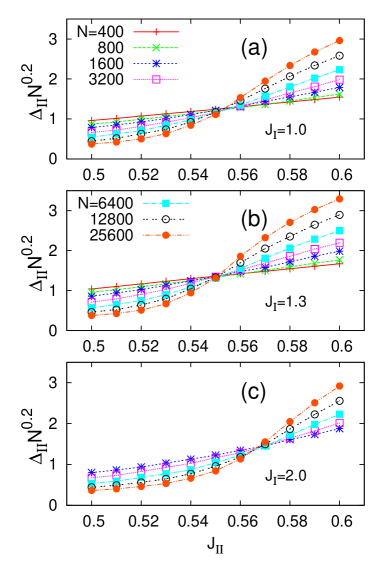
Figure 5: (Color online) Finite-size scaling [see Eq. (13)] for $\Delta_{\rm II}$ at $J=0.5$ and $J_{\rm I}=$ (a) 1.0, (b) 1.3, and (c) 2.0. Crossing point first decreases and then increases, indicating that there exists a reentrant transition.

To concrete our conclusion, we perform the FSS for $\Delta_{\rm II}$ as a function of $J_{\rm II}$ with varying $J_{\rm I}$, as shown in Fig. 5. Since $N^{\beta/\bar{\nu}}\Delta_{\rm II}=f(0)$ at $J_{\rm II}=J_{c}^{\rm II}$ from Eq. (13), crossings shown in Fig. 5 clearly manifest the reentrance behavior of $J_{c}^{\rm II}$: The crossing point decreases as $J_{\rm I}$ is increased from 1.0 to 1.3, and then increases as $J_{\rm I}$ is increased to 2.0. We report $J_{c}^{\rm II}$ obtained from FSS for $J=0.5$ in Fig. 6: $J_{c}^{\rm II}(J_{\rm I})$ first decreases from $J_{\rm I}=0$ as predicted in Sec.III.2, and makes an up turn before eventually decreases again for larger $J_{\rm I}$, consistent with Fig. 4. Here, we emphasize that the reentrance behavior of the onset develops at $J_{\rm I}>J$.

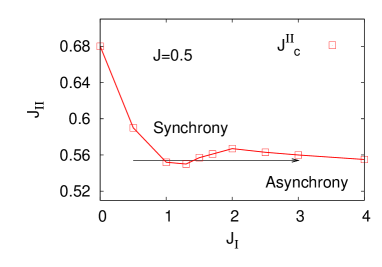
Figure 6: (Color online) Phase boundary at $J=0.5$ separating the synchronous (the upper region) and the asynchronous (the lower region) phases. Points are obtained from the FSS of $\Delta_{\rm II}$ [see Fig. 5]. As $J_{\rm I}$ is increased from below at $J_{\rm II}\approx 0.56$, the system starts from asynchronous phase, enters the synchronous phase, and then reenters back to the asynchronous phase as noted by the horizontal arrow.

The hump structure of the synchronization onset at $J_{\rm I}>J$ in Fig. 6 can be understood qualitatively by recalling the MF theory for $J_{c}^{\rm II}$ at $J_{\rm I}>J$ [see Eq. (11)], given by a function of fluctuations of frequency in clusters, $J_{c}^{\rm II}(J_{\rm I})\sim\sqrt{\bar{\sigma}^{2}_{\rm I}+\bar{\sigma}^{2}_{\rm II}}$. Rewriting Eq. (11) as

$$J_{c}^{\rm II}(J_{\rm I})\sim\sqrt{\left(N_{c}/N\right)\left(\mathcal{N}_{\rm I}^{-1}\sigma^{*2}_{\rm I}+\mathcal{N}_{\rm II}^{-1}\sigma^{*2}_{\rm II}\right)},$$ (14)

with $\sigma^{*2}_{\rm I(II)}=\mathcal{N}^{-1}_{\rm I(II)}\int_{-J_{\rm I}(-J)}^{J_{\rm I}(J)}d\omega_{\rm I(II)}\omega^{2}_{\rm I(II)}g(\omega_{\rm I(II)})$ and $\mathcal{N}_{\rm I(II)}=\int_{-J_{\rm I}(-J)}^{J_{\rm I}(J)}d\omega_{\rm I(II)}g(\omega_{\rm I(II)})$, one can find ingredients that determine the onset: For fixed $J$, $\mathcal{N}_{\rm II}^{-1}\sigma^{*2}_{\rm II}$ is constant, while $\mathcal{N}_{\rm I}^{-1}\sigma^{*2}_{\rm I}$ is an increasing function of $J_{\rm I}$. It is expected that as $J_{\rm I}$ is increased, $N_{c}$ increases at small $J_{\rm I}$ since clusters are created rather than merged. For large $J_{\rm I}$, on the other hand, $N_{c}$ should decrease as distinct clusters are merged.

We finally perform numerical RG analysis for the 1D regular network as described in Sec. III.3: Initially, the Gaussian frequency is distributed for a 1D network of the size $N$ up to $10^{6}$, and oscillators with $|\omega_{\rm I}|>J_{\rm I}$ are removed together with their bonds. Collecting fragments of the network, we calculate $N_{c}$ as a function of $J_{\rm I}$. From the numerical RG analysis, we find that $N_{c}/N$ as a function of $J_{\rm I}$ exhibits a well-defined peak near $J_{\rm I}\approx 0.45$ as seen in Fig. 7. This allows us to expect that $J_{c}^{\rm II}(J_{\rm I})$ has a peak at $J^{*}_{\rm I}$ slightly larger than $0.45$ since $\sigma^{*}_{\rm I}$ in the right-hand side of Eq. (14) is also an increasing function of $J_{\rm I}$. Since the expression for $J_{c}^{\rm II}$ in Eq. (14) is valid only for $J_{\rm I}>J$, for larger $J$ than $J^{*}_{\rm I}$, the reentrance behavior disappears as $J$ is increased further, as seen in Fig. 4. Although the values of $J_{\rm I}$ where the hump structure develops are different from those from the numerical investigation, the MF result made in Eq. (14) gives us a qualitatively correct prediction. It indicates that when $N_{c}$ increases with increasing $J_{\rm I}$, the synchronization in the WS network becomes worse since 1D clusters with different frequencies would act as burdens, while the merging of clusters yields the better synchronization for sufficiently large $J_{\rm I}$.

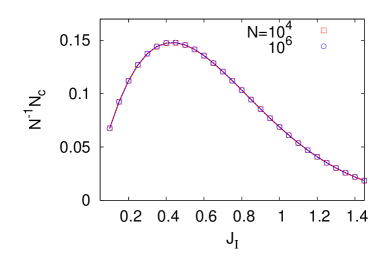
Figure 7: (Color online) Numerical RG calculation of $N_{c}/N$ as a function of $J_{\rm I}$ in the 1D regular network with $\langle k\rangle=4$. One thousand different sets of intrinsic frequencies are used for the average.

V Summary

We have investigated synchronization phenomenon in the interdependent two coupled networks; one is the 1D regular network and the other is the WS small-world network. Both the mean-field approximation and the numerical simulations have shown that the effect of the internetwork coupling is two folds: it suppresses the synchronization in the WS network when the 1D network is in the weak-coupling regime, while it enhances the synchronization in the strong-coupling regime. In comparison, the intranetwork coupling in the 1D network has been shown to always play a positive role in the synchronizability of the WS network. In the intermediate range of the intranetwork coupling, the reentrant behavior has been found numerically and explained within the MF scheme combined with the numerical RG calculations.

References

- (1) A. T. Winfree, The Geometry of Biological Time (Springer-Verlag, Berlin, 1980).
- (2) A. S. Pikovsky, M. Rosenblum, and J. Kurths, Synchronization: A Universal Concept in Nonlinear Science (Cambridge University Press, Cambridge, 2001).
- (3) S. Boccaletti, V. Latora, Y. Moreno, M. Chavez, and D.-U. Hwang, Phys. Rep. 424, 175 (2006).
- (4) Y. Kuramoto, in Proceedings of the International Symposium on Mathematical Problems in Theoretical Physics, edited by H. Araki (Springer, Berlin, 1975); Chemical Oscillations, Waves, and Turbulence (Springer, Berlin, 1984).
- (5) L. M. Pecora and T. L. Carroll, Phys. Rev. Lett. 80, 2109 (1998); M. Barahona and L. M. Pecora, ibid. 89, 054101 (2002); H. Hong, B. J. Kim, M. Y. Choi, and H. Park, Phys. Rev. E 69, 067105 (2004); S. M. Park and B. J. Kim, ibid. 74, 026114 (2006); T. Nishikawa and A. E. Motter, ibid. 73, 065106(R) (2006); J. Um, B. J. Kim, and S.-I. Lee, J. Korean Phys. Soc. 53, 491 (2008); S.-W. Son, B. J. Kim, H. Hong, and H. Jeong, Phys. Rev. Lett. 103, 228702 (2009);R. Tönjes, N. Masuda, and H. Kori, Chaos 20, 033108 (2010).
- (6) J. Gómez-Gardeñes, Y. Moreno, and A. Arenas, Phys. Rev. Lett. 98, 034101 (2007); Phys. Rev. E 75, 066106 (2007).
- (7) H. Hong, M. Y. Choi, and B. J. Kim, Phys. Rev. E 65, 026139 (2002).
- (8) J. G. Restrepo, E. Ott, and B. R. Hunt, Phys. Rev. E 71, 036151 (2005); Chaos 16, 015107 (2005).
- (9) H. Hong, H. Park, and L.-H. Tang, Phys. Rev. E 76, 066104 (2007).
- (10) H. Hong, H. Park, and M. Y. Choi, Phys. Rev. E 70, 045204(R) (2004); 72,036217 (2005).
- (11) H. Hong, H. Chate, H. Park, and L.-H. Tang, Rhys. Rev. Lett. 99, 184101 (2007).
- (12) P. Erdös and A. Rényi, Publicationes Mathematicae Debrencen 6, 290 (1959).
- (13) D. J. Watts and S. H. Strogatz, Nature (London) 393, 440 (1998).
- (14) S. V. Buldyrev, R. Parshani, G. Paul, H. E. Stanley, and S. Havlin, Nature 464, 1025 (2010).
- (15) For more examples, S. Havlin, N. A. M. Araujo, S. V. Buldyrev, C. S. Dias, R. Parshani, G. Paul, and H. E. Stanley, arXiv:1012.0206v1.
- (16) R. Parshani, S. V. Buldyrev, and S. Havlin, Phys. Rev. Lett. 105, 048701 (2010); Proc. Natl. Aca. Sci. (USA) 108, 1007 (2011).
- (17) H. -H. Jo, S. K. Baek, and H. -T. Moon, Physica A 361, 534 (2006).
- (18) P. A. Robinson, C. J. Rennie, and D. L. Rowe, Phys. Rev. E 65, 041924 (2002); J. D. Victor, J. D. Drover, M. M. Conte, and N. D. Schiff, Proc. Natl. Aca. Sci. (USA) (in press) (doi:10.1073/pnas.1012168108).
- (19) O. Kogan, J. L. Rogers, M. C. Cross, and G. Refael, Phys. Rev. E 80, 036206 (2009); T. E. Lee, G. Rafael, M. C. Cross, O. Kogan, and J. L. Rogers, ibid. 80, 046210 (2009).