Subaru weak-lensing study of A2163: bimodal mass structure

Abstract

We present a weak-lensing analysis of the merging cluster A2163 using Subaru/Suprime-Cam and CFHT/Mega-Cam data and discuss the dynamics of this cluster merger, based on complementary weak-lensing, X-ray, and optical spectroscopic data sets. From two-dimensional multi-component weak-lensing analysis, we reveal that the cluster mass distribution is well described by three main components including a two component main cluster A2163-A with mass ratio 1:8, and its cluster satellite A2163-B. The bimodal mass distribution in A2163-A is similar to the galaxy density distribution, but appears as spatially segregated from the brightest X-ray emitting gas region. We discuss the possible origins of this gas-dark matter offset, and suggest the gas core of the A2163-A subcluster has been stripped away by ram pressure from its dark matter component. The survival of this gas core to the tidal forces exerted by the main cluster lets us infer a subcluster accretion with a non-zero impact parameter. Dominated by the most massive component of A2163-A, the mass distribution of A2163 is well described by a universal Navarro-Frenk-White profile as shown by a one-dimensional tangential shear analysis, while the singular-isothermal sphere profile is strongly ruled out. Comparing this cluster mass profile with profiles derived assuming intracluster medium hydrostatic equilibrium (H.E.) in two opposite regions of the cluster atmosphere has allowed us to confirm the prediction of a departure from H.E. in the eastern cluster side, presumably due to shock heating. Yielding a cluster mass estimate of $M_{500}=11.18_{-1.46}^{+1.64}\times 10^{14}h^{-1}M_{\odot}$, our mass profile confirms the exceptionally high mass of A2163, consistent with previous analyses relying on the cluster dynamical analysis and $Y_{\rm X}$ mass proxy.

1. Introduction

Galaxy clusters are the largest self-gravitating systems in the universe, residing at the intersection of large-scale filamentary structures of the cosmic web. According to the hierarchical structure formation scenario based on a cold dark matter (CDM) paradigm, mass accretion flows onto clusters are still ongoing and high-mass ratio cluster mergers, the so-called major mergers, sometimes occur. Major cluster mergers are among the most energetic events in the universe, releasing amounts of gravitational energy as large as $10^{64-65}{\rm erg}$. Spatially resolved X-ray observation has revealed to us that this collision energy partly dissipates in the intracluster medium (ICM) through shock heating and turbulence, yielding a complex ICM brightness and thermal structure (see, e.g., Markevitch & Vikhlinin, 2007, and reference therein). The dynamics of cluster collisions are however dominated by the cluster mass distribution, which cannot be constrained from X-ray observations alone. Due to the collisional nature of ICM, cluster mergers are indeed expected to generate some transient decoupling between spatial distributions of the CDM and hot X-ray emitting gas. Moreover, mass estimates relying on gas properties may be biased by merger-induced perturbations of the ICM hydrostatic equilibrium (H.E.) within individual colliding clusters.

Weak-lensing distortions of background galaxy images provide us with a unique opportunity to reconstruct the distribution of matter in clusters without any assumption of mass model and dynamical states (e.g., Kaiser et al., 1995; Bartelmann & Schneider, 2001; Schneider, 2006; Okabe & Umetsu, 2008; Okabe et al., 2010b) and measure cluster masses (e.g., Gray et al., 2002; Gavazzi et al., 2003; Bardeau et al., 2007; Hoekstra, 2007; Okabe et al., 2010b; Umetsu et al., 2009). Therefore, a weak-lensing analysis of merging clusters (e.g., Clowe et al., 2006; Mahdavi et al., 2007; Okabe & Umetsu, 2008; Okabe et al., 2010b; Merten et al., 2011) is an observational breakthrough in measuring mass distribution, thereby providing complementary information to X-ray measurements. Okabe & Umetsu (2008) conducted a systematic study of seven merging clusters, representing various merging stages and conditions, based on a joint weak-lensing, optical photometric, and X-ray analysis, and revealed that the mass and optical light of member galaxies are similarly distributed in merging clusters regardless of their merging stages, but the mass distribution in merging clusters is highly irregular, and is quite different from the ICM distributions. It indicates that the gas and mass evolutions under cluster mergers are different. This feature is confirmed by weak-lensing studies of 30 clusters as a collaboration of “Local Cluster Substructure Survey” (Okabe et al., 2010b). Thus, a joint analysis of clusters (e.g., Mahdavi et al., 2008; Okabe & Umetsu, 2008; Okabe et al., 2010c; Kawaharada et al., 2010; Umetsu et al., 2010; Zhang et al., 2010) will yield a comprehensive and quantitative understanding of cluster merger physics involved in the structure formation.

Located at a redshift of $0.203$, A2163 is a rich, X-ray luminous and hot galaxy cluster showing various signatures of ongoing merger events, including irregular optical and X-ray morphologies (see, e.g. Elbaz et al., 1995; Markevitch & Vikhlinin, 2001; Maurogordato et al., 2008; Bourdin et al., 2011), and a prominent radio halo emission (Feretti et al., 2001, 2004). This cluster has been known to exhibit a clear spatial segregation between a bimodal galaxy distribution and a more centrally peaked ICM morphology (Maurogordato et al., 2008, hereafter M08), while the projected distance separating its main mass and gas centroids has been measured as one of the largest in a sample of 38 clusters analyzed from both strong galaxy lensing and X-ray imaging (Shan et al., 2010). As revealed from spectroscopic and photometric analyses in M08, the galaxy distribution in A2163 can be separated into two components: the massive cluster A2163-A and its northern companion A2163-B, and the main cluster component itself showing a bimodal morphology with two brightest galaxies (BCG1 and BCG2). In a more recent analysis of Chandra and XMM-Newton data, Bourdin et al. (2011, hereafter B11) evidenced the westward motion of a cool core across the E-W elongated atmosphere of the main cluster, A2163-A. Located close to the second galaxy over-density, this gas ’bullet’ appears to have been spatially separated from its galaxy component as a result of high-velocity accretion. From gas brightness and temperature profile analysis performed in two opposite regions of the main cluster, B11 further showed that the ICM has been adiabatically compressed behind this crossing “bullet”.

Characterized by an exceptionally high ICM temperature first measured in X-ray ($k_{B}T=13.9$ keV; Arnaud et al., 1992) then confirmed from its Sunyaev-Zeldovich (SZ) distortion (Nord et al., 2009), A2163 has been suggested to be exceptionally massive from various X-ray and SZ analyses (see, e.g. Vikhlinin et al., 2009a; Planck Collaboration, 2011) via the mass scaling relation. Former weak-lensing analyses have been conducted using the Very Large Telescope and CFHT/Mega-Cam analyses of Cypriano et al. (2004) and Radovich et al. (2008). These analyses, however, did not exclude merger galaxies in the background shear catalog, as demonstrated by other studies (Broadhurst et al., 2005; Okabe & Umetsu, 2008; Umetsu & Broadhurst, 2008; Umetsu et al., 2009; Okabe et al., 2010b; Umetsu et al., 2010). As shown by Okabe et al. (2010b), a contamination of member galaxies significantly dilutes lensing distortion signals, mainly in the central region, thereby yielding biased estimations on cluster parameters.

In this paper, we conducted a weak-lensing analysis using Subaru/Suprime-Cam and made a secure selection to avoid a contamination of member galaxies in the shear catalog, combining CFHT/Mega-Cam data. The structure of this paper is as follows: in Section 2 we briefly describe the weak-lensing analysis. The projected distributions of mass, member galaxies and hot-gas are compared in Section 3. Section 4 is devoted to a one-dimensional shear analysis to measure cluster mass. In Sec 5, we perform, based on a two dimensional shear pattern, a multi-components fitting to measure three components revealed by M08. We compare weak lensing mass with dynamical and X-ray hydrostatic equilibrium masses in Section  6. In Section  7, we discuss quantitatively the physical process of making an offset between mass and gas distributions. Section  8 summarizes our results. The cosmological parameters of $H_{0}=100h^{-1}$ Mpc^-1 km s^-1, $\Omega_{0}=0.3$, and $\Lambda_{0}=0.7$ are used in this paper. Given the cosmology, $1\farcm=140.21~{}h^{-1}{\rm kpc}$.

2. Data Analysis

We retrieved $R_{\rm c}$ image data from the Subaru archival data (SMOKA). The data were reduced by the standard imaging process of using the reduction software for Suprime-Cam, SDFRED (Ouchi et al., 2004), as described in Okabe & Umetsu (2008) and Okabe et al. (2010b). Astrometry calibration was conducted by fitting the final stacked image with the Two Micron All Sky Survey data catalog. The residual in astrometric fitting was lower than the CCD pixel size. The exposure time is $75$ minutes and the seeing is $0\farcs 79$; therefore, it is suitable for our weak-lensing study. Since no other band data are available, we use CFHT/Mega-cam $g^{\prime}$ imaging data to exclude unlensed galaxies in the shear source catalog via a color-magnitude plane.

Our weak-lensing analysis is done using the IMCAT package provided by N. Kaiser (Kaiser et al. 1995). We use the same pipeline as Okabe et al. (2010a, b) with some modifications followed by Erben et al. (2001). We first measure the image ellipticity, $e_{\alpha}$, from the weighted quadrupole moments of the surface brightness of each object and then correct the point-spread function (PSF) anisotropy by solving $e_{\alpha}^{\prime}=e_{\alpha}-P_{\rm sm}^{\alpha\beta}(P_{\rm sm}^{*})^{-1}_{\beta\gamma}e^{\gamma*}$, where $P_{\alpha\beta}$ is the smear polarizability tensor and the asterisk denotes the stellar objects. We fit the stellar anisotropy kernel $(P_{\rm sm}^{*})^{-1}_{\alpha\beta}e^{\beta*}$ with the second-order bi-polynomials function in several subimages whose sizes are determined based on the typical coherent scale of the measured PSF anisotropy pattern. The median stellar ellipticities before and after the anisotropic correction are $(\bar{e}_{1}^{*},\bar{e}_{2}^{*})=(1.45\pm 0.02,1.52\pm 0.01)\times 10^{-2}$ and $(\bar{e}_{1}^{\rm res,*},\bar{e}_{2}^{\rm res,*})=(-3.74\pm 5.30,-5.07\pm 4.73)\times 10^{-5}$, respectively. Stellar ellipticities before and after the correction and their pattern are shown in Figures 1 and 2, respectively. We next estimate the reduced shear $g_{\alpha}=\gamma_{\alpha}/(1-\kappa)=(P_{g})_{\alpha\beta}^{-1}e_{\beta}^{\prime}$ using the pre-seeing shear polarizability tensor $P_{g}$, where we adopt the scalar value $(P_{g})_{\alpha\beta}={\rm Tr}[P_{g}]\delta_{\alpha\beta}/2$. We select background galaxies in the range of ${\bar{r}}_{h}^{*}+\sigma_{r_{h}^{*}}<r_{h}<r_{h,\rm max}\simeq 6.6~{}{\rm pixels}$, where $r_{h}$ is the half-light radius, and ${\bar{r}}_{h}^{*}$ and $\sigma_{r_{h}^{*}}$ are the median and standard error of stellar half-light radii, $r_{h^{*}}$, corresponding to the half median width of circularized PSF. Then, we make a secure selection of background galaxies in a color-magnitude plane in order to minimize a dilution of the weak-lensing signals caused by a contamination of unlensed galaxies, mainly member galaxies. As shown in Okabe et al. (2010b), the dilution effect on the lensing signals is more pronounced at smaller radii because the ratio of the number density of cluster galaxies to background ones rises towards the inner region. We use Subaru/Suprime-Cam $R_{\rm c}$ and CFHT/Mega-cam $g^{\prime}$ images. The difference in filter sensitivity functions of the wavelength in the $g^{\prime}$ band between these two instruments is negligible. Therefore, a combination with Subaru and CFHT enables us to efficiently exclude member galaxies inthe background shear catalog. Following Umetsu & Broadhurst (2008), we calculate the lensing signal as a function of color (Figure 3), by averaging the tangential distortion strengths (see also Okabe et al., 2010b). We securely select background galaxies in the range of $0.82<(R_{\rm c}-g^{\prime})-(R_{\rm c}-g^{\prime})_{{\rm RS}}<2$, $-2<(R_{\rm c}-g^{\prime})-(R_{\rm c}-g^{\prime})_{{\rm RS}}<-0.38$ and $22~{}{\rm ABmag}<R_{\rm c}$, where $(R_{\rm c}-g^{\prime})_{{\rm RS}}$ is the best-fit linear function as a magnitude $R_{\rm c}$ of red-sequence galaxies; $(R_{\rm c}-g^{\prime})_{{\rm RS}}=-0.056R_{\rm c}+2.812$, as shown in Figure 4. Here, the magnitudes and colors are measured by MAG_AUTO (i.e., total magnitude) and MAG_APER (i.e., aperture magnitude) in SExtractor, respectively. By a selection in the color magnitude plane, the number density of background galaxies in the shear catalog decreases from $\simeq 23$ to $\simeq 12~{}\rm arcmin^{-2}$. The mean redshift of these background galaxies is estimated by matching the COSMOS catalog (Ilbert et al., 2009) to calculate the average lensing weight $\langle D_{\rm ls}/D_{\rm s}\rangle=\int_{z_{d}}dzdP_{\rm WL}/dzD_{\rm ls}/D_{\rm s}$, where $D_{\rm s}$ and $D_{\rm ls}$ are the angular diameter distances between the observer and source (background galaxy) and lens and source, respectively, and $dP_{\rm WL}/dz$ is a probability function of redshift distribution. We obtain $\langle D_{\rm ls}/D_{\rm s}\rangle\simeq 0.7209$.

3. Maps of Mass, Galaxies and Gas

According to the CDM paradigm, the collisional ICM is expected to experience a spatial decoupling from galaxies and dark matter during cluster collisions. Comparing hot X-ray emitting gas maps with the cluster member galaxy density and mass distributions has thus been known to testify to the merging cluster dynamical states (see, e.g. Clowe et al., 2006; Okabe & Umetsu, 2008). In order to investigate the collision scenario in A2163, we map out the cluster mass distribution and compare it with spatial distributions of the galaxy and hot gas components.

As described in detail in Okabe & Umetsu (2008), we pixelize the shear pattern into a regular grid using Gaussian smoothing kernel $w_{g}(\theta)\propto\exp[-\theta^{2}/\theta_{g}^{2}]$ with $\theta_{g}={\rm FWHM}/\sqrt{4\ln{2}}$. We adopt the smoothing scale of ${\rm FWHM}=1\farcm 33$ due to the limitation of the number of background galaxies. We also use a statistical weight for each background galaxy in the context of

$$u_{g,i}=\frac{1}{\sigma_{g,i}^{2}+\alpha^{2}},$$ (1)

where $\sigma_{g,i}$ is the rms error for shear measurement of $i$th galaxy and $\alpha$ is the softening constant variance. We set $\alpha=(\sum\sigma_{g,i}^{2}/N)^{1/2}\simeq 0.44$. The reduced shear at pixel position of $\mbox{\boldmath$\theta$}_{n}$ is obtained by

$$\langle{g_{\alpha}}\rangle(\mbox{\boldmath$\theta$}_{n})=\frac{\sum_{i}w_{g}(\mbox{\boldmath$\theta$}_{n}-\mbox{\boldmath$\theta$}_{i})u_{g,i}g_{\alpha,i}}{\sum_{i}w_{g}(\mbox{\boldmath$\theta$}_{n}-\mbox{\boldmath$\theta$}_{i})u_{g,i}}.$$ (2)

Then, we invert the pixelized reduced shear (Equation 2) with a weight of the inverse of the variance at each pixel to the lensing convergence field, based on the Kaiser & Squires inversion method (Kaiser & Squires, 1993).

We also map out distributions of optical luminosities and the number density of member galaxies with the same kernel with $u_{g}=1$. The luminosity and density maps are sensitive to luminous and high-density structures, respectively. We selected red-sequence galaxies with $R_{\rm c}<22{\rm ABmag}$ as member galaxies. The absolute magnitudes for member galaxies are calculated from the apparent magnitude using the $k$-correction for early-type galaxies. We assume that all cluster member galaxies in the catalog are at a single redshift.

The resultant lensing $\kappa$ field is shown in Figures 5 and 6, with contours equi-spaced in units of $1\sigma$ reconstruction error, $\delta\kappa=0.0404$, above the $1\sigma$ level. This mass distribution clearly exhibit a bimodal morphology in the central region ($r\sim 3\farcm$), with two peaks reaching significance levels of $\sim 10\sigma$ and $\sim 5.6\sigma$, respectively. Interestingly, these two peaks coincide with the two galaxy overdensities A1 and A2 hosting the two brightest cluster galaxies revealed in M08, BCG1, and BCG2 (see also the top right and bottom left panels of Figure 6). We hereafter refer to these primary and secondary mass peaks as MC and MW, respectively. The cluster mass distribution further exhibits some anisotropies at larger radii, mostly coinciding with peripheral optical clumps first revealed in M08 and presently confirmed (see the bottom left panel of Figure 6). The most significant of these coinciding mass and optical peaks is $\sim 3.3\sigma$ at the optical clump, B.

The mass distribution in the region of optical substructures C, D, and E, discovered by M08, is similar to those of the number and luminous density, albeit low significance levels (Table 1). We measure luminosities within $2\farcm$ centering each $\kappa$ peak (Table 1), where a background region of $20-22\farcm$ centering BCG1 is used. We find that luminosities and signal-to-noise ratios of $\kappa$ are correlated. We tried to measure model-independent mass for each optical subclump, following Okabe et al. (2010a). However, since the result is sensitive to the choice of background region, we could not obtain reliable results. An over-density region is further revealed from the density of galaxies whose colors are redder by $\sim 0.6$ at $R_{\rm c}=22~{}{\rm ABmag}$ (see the bottom right panel of Figure 6). The width of colors for these galaxies is $\sim 0.15$. Distributed at the west of A2163, these optical structures are associated with mass clumps of $\sim 2-3\sigma$. More generally speaking, the cluster mass distribution appears as spatially correlated with density distribution of its member galaxies, consistently with weak-lensing studies in other clusters (Okabe & Umetsu, 2008; Okabe et al., 2010b).

We next compare the cluster mass contours with X-ray surface brightness and temperature maps derived from XMM-Newton and Chandra data analysis in B11. The left panel of Figure 7 shows us a wavelet denoised map of the overall cluster atmosphere, with mass contours superimposed. These two distributions clearly exhibit a spatial segregation, the X-ray emission appearing as unimodal and E-W elongated, with an emission peak located between the two mass peaks. The right panel of Figure 7 shows high-resolution details in a multi-resolution analysis of the Chandra image. This analysis reveals a secondary cluster X-ray core, XW, separated from the main cluster emission peak, XC. As shown in B11, this wedge-shaped feature (red-curved line in the right panel of Figure 7) appears as a stripped cool core embedded in the hotter ICM of A2163-A and delimited in the westward direction by a cold front. The evidence of this cold front let us infer the westward motion of this gas ’bullet’ along the elongated atmosphere of A2163-A. Interestingly, we now observe that the crossing core appears as preceded by the secondary mass peak, from which it might have been spatially separated during a subcluster accretion onto the main cluster. This offset feature between the X-ray clump and mass peak is consistent with other cold front clusters on a merging phase (Clowe et al., 2006; Okabe & Umetsu, 2008; Okabe et al., 2010b). It suggests a possibility of ram pressure stripping of the accreted cluster core (see also Section 7).

It is further worth noticing that the main cluster mass peak, MC, also appears as slightly offset from the X-ray core, XC, so that the centroid of the gas core of XC and XW is at the intermediate position between the two mass peaks. This ‘double offset’ separating the gas and dark matter contents of both the infalling and main cluster cores presents some similarities to the fast accretion observable in 1E0657-56 (Clowe et al., 2006), the so-called “bullet-cluster”. To our knowledge, no other bimodal merger has been known so far to exhibit such a significant offset between the gas and dark matter components of its two components (see, e.g. other examples in Okabe & Umetsu, 2008).

The northern subcluster A2163-B exhibits a spatial coincidence between X-ray, mass, and member galaxies, consistent with what is usually observed in pre-merging systems (Okabe & Umetsu, 2008). Consistent with the lack of any interaction evidence found from ICM thermodynamics between A2163-A and A2163-B, this spatial coincidence suggests that A2163-B is likely to be observed before interacting with A2163-A.

4. Tangential distortion Analysis

We conduct a tangential distortion study, which is a one-dimensional lensing analysis, in order to measure the total cluster mass. The tangential distortion component of the reduced shear, $g_{\alpha}=(g_{1},g_{2})$, and the $45$ degree rotated component for individual galaxies ($i$th galaxy) are obtained by

$$g_{+,i} = -g_{1,i}\cos 2\varphi-g_{2,i}\sin 2\varphi,$$

$$g_{\times,i} = -g_{1,i}\sin 2\varphi+g_{2,i}\cos 2\varphi,$$ (3)

where $\varphi$ is the position angle in the counter clockwise direction from the first coordinate axis on the sky. Then, the profiles of $g_{+}$ and $g_{\times}$ are estimated with a statistical weight (Equation 1), as follows:

$$\langle{g_{\alpha}}\rangle(\theta_{n})=\frac{\sum_{i}u_{g,i}g_{\alpha,i}}{\sum_{i}u_{g,i}}.$$ (4)

Here, $n$ denotes the $n$th radial bin $\theta_{n}$ with a given bin. The statistical error of $g_{\alpha}$ in each radial bin is estimated as

$$\sigma_{g_{\alpha}}^{2}(\theta_{n})=\frac{1}{2}\frac{\sum_{i}u_{i}^{2}\sigma_{g,i}^{2}}{\left(\sum_{i}u_{i}\right)^{2}},$$ (5)

where the prefactor $1/2$ comes from the fact that $\sigma_{g,i}$ in the rms is the sum of two distortion components.

We fit the tangential distortion profile with the universal profile proposed by Navarro, et al. (1996, hereafter NFW profile) and a singular isothermal sphere (SIS) halo model. The NFW halo mass is a prediction of numerical simulations based CDM model. The mass density profiles over a wide range of masses are well described in the form of

$$\rho_{\rm NFW}(r)=\frac{\rho_{s}}{(r/r_{s})(1+r/r_{s})^{2}},$$ (6)

where $\rho_{s}$ is the central density parameter and $r_{s}$ is the scale radius. The asymptotic inner and outer slopes for NFW mass density are $\rho\propto r^{-1}$ and $r^{-3}$, respectively. The three-dimensional mass profile within a radius, $r_{\delta}$, at which the mean density is $\Delta$ times the critical mass density, $\rho_{\rm cr}(z)$, at the cluster redshift, is expressed by

$$M_{\rm NFW}(<r_{\Delta})=\frac{4\pi\rho_{s}r_{\Delta}^{3}}{c_{\Delta}^{3}}m(c_{\Delta}),$$ (7)

with

$$m(x) = \log(1+x)-\frac{x}{1+x}.$$ (8)

The NFW halo mass is described by two parameters of the mass $M_{\rm NFW}(<r_{\Delta})$ and the halo concentration $c_{\rm\Delta}=r_{\Delta}/r_{s}$.

The SIS halo model is a solution of the collisionless Boltzmann equation, and is specified by one parameter, the one-dimensional velocity dispersion $\sigma_{v}^{2}$, as follows,

$$\rho_{\rm SIS}(r)=\frac{\sigma_{v}^{2}}{2\pi G}\frac{1}{r^{2}}.$$ (9)

A three-dimensional mass for the SIS model is given by

$$M_{\rm SIS}(<r_{\Delta}) = \frac{2\sigma_{v}^{2}}{G}r_{\Delta}.$$ (10)

The tangential distortion profile and the best-fit models are shown in Figure 8. We choose the central position determined by two-dimensional shear analysis which will be described in detail in Section 5. We also measure the tangential shear profile with a center of BCG1 and fit them, but the results do not change significantly. We can clearly find a curvature of the tangential shear profile. The curvature makes it difficult to fit the profile with the SIS model. The $\chi^{2}{\rm(d.o.f)}$ for the SIS model is $27.85(7)$; therefore, the SIS model can be strongly rejected ($5\sigma$ level) as a mass model. On the other hand, the NFW mass model well expresses the curvature of the profile. Indeed, $\chi^{2}$ for the NFW model is $0.82(6)$. The best-fit NFW parameters are found in Table 2. The virial mass shows the massive cluster, $M_{\rm vir}=24.25^{+6.00}_{-4.55}\times 10^{14}h^{-1}M_{\odot}$, where the virial overdensity is $\Delta_{\rm vir}\simeq 116.4$. Our mass estimates are larger than those of a previous weak-lensing study (Table 2; Radovich et al., 2008), using the shear catalog without excluding a contamination of member galaxies.

5. Two-Dimensional Shear Analysis

As shown in Figures 5 and 6, the projected mass distribution of A2163 is complex and two mass peaks are significantly detected in the central region. It is of prime importance for understanding cluster merger phenomena to measure masses of the main- and sub- clusters. Furthermore, since numerical simulations (Meneghetti et al., 2010; Becker & Kravtsov, 2010) and observations (Okabe et al., 2010b) have shown that a tangential shear profile is affected by significant substructures, taking into account substructures in modeling is also important for understanding such a lensing bias. In the mass measurement using the tangential shear profile (Section 4), it is very difficult to distinguish which structure contributes in part to the tangential distortion signals, because the full lensing information from both the main and subclusters must be convolved to express the one dimensional distortion profile with respect to a given center (Okabe et al., 2010a). The two dimensional shear pattern, on the other hand, enables us to easily model lensing signals by a superposition of lensing signals. In this section, we conduct two-dimensional shear fitting in order to measure the masses of three components (the sub and main components for A2163-A and A2163-B) revealed by M08 and B11.

We pixelize the shear pattern into a regular grid of $1\farcm\times 1\farcm$ without any spatial smoothing procedure, whereas we adopted Gaussian smoothing in the map making (Section 3). The pixelized distortion signals and statistical weight, $\langle{g_{\alpha}}\rangle(\mbox{\boldmath$\theta$}_{n})$ and $\sigma_{g}^{2}(\mbox{\boldmath$\theta$}_{n})$, in the $n$th pixel are estimated with a weight function $u_{i}$ for each background source residing in the pixel (see also Equations. (4) and (5)). The representative position for the $n$th pixel is also estimated with a weight function $u_{i}$. The $\chi^{2}$ fitting is given by

$$\chi^{2} = \sum\limits_{\alpha,\beta=1}^{2}\sum\limits_{n}^{N_{\rm pixel}}(g_{\alpha}(\mbox{\boldmath$\theta$}_{n})-g_{\alpha}(\mbox{\boldmath$\theta$}_{n};\mbox{\boldmath$p$})^{(\rm model)})C_{\alpha\beta}^{-1}(\mbox{\boldmath$\theta$}_{n})$$ (11)

$$(g_{\beta}(\mbox{\boldmath$\theta$}_{n})-g_{\beta}(\mbox{\boldmath$\theta$}_{n};\mbox{\boldmath$p$})^{(\rm model)}),$$

where $p$ is the parameters and $C_{\alpha\beta}$ is the error covariance matrix of shape measurements in the form of $C_{\alpha\beta}(\mbox{\boldmath$\theta$}_{n})=\delta^{\rm K}_{\alpha\beta}\sigma_{g}^{2}(\mbox{\boldmath$\theta$}_{n})$. Here, $\delta^{\rm K}_{\alpha\beta}$ is a Kronecker delta function and $\sigma_{g}^{2}(\mbox{\boldmath$\theta$}_{n})$ is the statistical error of the pixelized shear (Oguri et al., 2010; Watanabe et al., 2011).

We first consider a single mass model of the NFW profile in order to compare the mass estimates by tangential shear measurement. We here treat the center of NFW mass ($x_{c}$, $y_{c}$) as a parameter. In total, we use four parameters ($M$, $c$, $x_{c}$, and $y_{c}$) for fitting. We adopt the Markov Chain Monte Carlo method with standard Metropolis-Hastings sampling. We restrict the sampling range of $M_{\rm vir}\leq 5\times 10^{15}h^{-1}M_{\odot}$, $c_{\rm vir}\leq 20$. We refer to the mean of the posterior probability distribution of each parameter. The resultant masses are consistent with the tangential shear measurements (Table 2). The central position of mass is consistent with the peak position of the MC clump in the mass map. The MC clump, which is associated with BCG1, is therefore likely to be the main component.

We next add a mass model for the mass clump MW to the main cluster. From X-ray and optical spectroscopic studies (M08 and B11), the mass clump MW is likely to be a merging substructure in A2163-A. Since cluster substructure size is not determined by the virial theorem but by the strong tidal force of the main cluster (e.g., Tormen et al., 1998), we adopt the truncated SIS (TSIS) model (Okabe et al., 2010a) to describe the MW clump. The TSIS model is an extreme case of the truncation; mass density becomes zero at a radius $r_{t}$. The TSIS mass profile is expressed as

$$\rho_{\rm TSIS}(r) = \rho_{\rm SIS}(r)~{}~{}~{}~{}~{}~{}{\rm for}~{}~{}r\leq r_{t}$$

$$= 0~{}~{}~{}~{}~{}~{}~{}~{}~{}~{}~{}~{}~{}{\rm for}~{}~{}r>r_{t}.$$

The subclump mass for the TSIS model is estimated as

$$M_{\rm sub}^{\rm(TSIS)}=\frac{2\sigma_{v,t}^{2}}{G}r_{t}.$$ (13)

The TSIS model is specified by one-dimensional velocity dispersion $\sigma_{v}$ and the truncation radius $r_{t}$. We have an additional four parameters ($\sigma_{v}$, $r_{t}$ and centers) for the TSIS model and a total of eight parameters for the fitting. We assume that the redshift of the MW clump is the same as that of the main cluster. We adopt $|x_{c}-x_{\rm peak}|<2\farcm$ and $|y_{c}-y_{\rm peak}|<2\farcm$, where $x_{\rm peak}$ and $y_{\rm peak}$ are peak coordinates appearing in a weak-lensing mass map. The resultant mass and central positions are shown in Table 3. The centroid of the MW clump is consistent with the peak found in the mass map. The truncation radius, $r_{t}=9\farcm 7_{-2.9}^{+3.4}\sim 1.4h^{-1}{\rm Mpc}$, is an intermediate size compared to the virial radius of the main cluster $r_{\rm vir}=16\farcm 6\sim 2.3h^{-1}{\rm Mpc}$. Since the sub-cluster size after some impacts is significantly decreased by the strong tidal field, such a large truncation radius might suggest that the MW clump is a merging sub-cluster at the first impact.

Next, we take into account the northern component A2163-B (M08 and B11 ), which contains luminous galaxies (optical clump B) and an X-ray emitting core. We consider two possibilities for the dynamic state of A2163-B; one scenario is the pre-merger phase that A2163-B is infalling toward A2163-A, and the other is that A2163-B has already undergone a merging event with the main cluster of A2163-A. B11 found no evidence of the close interaction between A2163-A and A2163-B, and therefore concluded that they are likely to be separated more than $r_{500}$ aligning along the line of sight. However, in M08, a filament of faint galaxies was detected along a north/south axis between A2163-A and A2163-B which might suggest a previous interaction between the two components. Although this post-merger hypothesis is very unlikely from the X-ray approach, the origin of this faint galaxy filamentary structure is still an open issue. In this paper, we investigate two possibilities in the fitting. If A2163-B is physically separated from A2163-A, its mass profile is not likely to be affected by the strong tidal field of A2163-A and we therefore adopt the NFW model for the first scenario. Here, the halo concentration is ill constrained because the shear signals from A2163-B are smaller than those from A2163-A, and it is difficult in the environment of the massive cluster to find the curvature of the distortion profile, as shown in Figure 8. We therefore assume the mass - concentration relation of $c_{\rm vir}=7.85\left(M_{\rm vir}/2\times 10^{12}h^{-1}M_{\odot}\right)^{-0.081}(1+z_{c})^{-0.71}$ (Duffy et al., 2008). Here, we assume a redshift of A2163-B, $z_{c}$, is the same as that of A2163-A. This assumption is justified by both the dynamical analysis (M08) and the photometric redshift estimates by La Barbera et al. (2004). We also parameterize the center of A2163-B, using 13 parameters in total. The resultant virial mass is $M_{\rm vir,B}=2.43_{-1.15}^{+0.90}\times 10^{14}h^{-1}M_{\odot}$ (Table 3). The mass $M_{500,\rm B}=1.34_{-0.64}^{+0.49}\times 10^{14}h^{-1}M_{\odot}$ within a radius $r_{500}$, at which the mean density is $500$ times the critical density, agrees well with X-ray estimates $M_{500,B}=(1.47\pm 0.07)\times 10^{14}h^{-1}M_{\odot}$ (B11). We changed the normalization of the mass -concentration relation by $\pm 2$ and conducted fittings, but the best fit of the virial mass for A2163-B changes only by $+14\%$ and $-10\%$. They all are consistent within errors. We also found that the MC and MW masses are almost unchanged after adding the mass model of A2163-B. The resultant mass ratios of MC (main cluster of A2163-A), MW (sub cluster of A2163-A) and A2163-B are found to be $\sim 8:1:1$.

We consider the second scenario that A2163-B is an ongoing merger with A2163-A. We here use the TSIS model for A2163-B, following the case of the substructure MW. The truncation radius $r_{t}=741.3^{+289.1}_{-342.8}~{}{\rm kpc}h^{-1}$ is obtained, while the concentration of the NFW mass model is not well constrained. This is because the tangential distortion profile for the truncation model outside the truncation radius is proportional to the inverse square of the radius ($g_{+}\propto r^{-2}$), which is different from that of the NFW mass model for the main cluster. We obtain the substructure mas $M_{\rm B}=1.44_{-0.84}^{+0.64}\times 10^{14}h^{-1}M_{\odot}$. The mass discrepancy between the two models is small: $0.9\sigma$ and $1.2\sigma$ with uncertainties of NFW and TSIS masses, respectively. The two mass models (NFW and TSIS) obtained solely by shear data are, therefore, acceptable for A2163-B. The total mass in each model is consistent within errors with tangential shear measurement, which indicates that a substructure effect is likely to be less significant.

6. Mass Comparisons

Due to its exceptionally high mass and dynamical activity, A2163 has long been an interesting test case for cluster mass measurements. We here compare the weak lensing cluster mass, $M_{\rm vir}=24.24^{+6.00}_{-4.55}\times 10^{14}h^{-1}M_{\odot}$ (see Section 4 and Figure  9), with dynamical and X-ray mass estimates provided by M08 and B11. As previously mentioned, weak lensing mass measurements do not require any assumption of cluster dynamical state. They consequently provide us a unique opportunity to investigate effects of the virial theorem hypothesis for member galaxies or the gas H.E. assumption on mass measurement precision.

6.1. Mass estimate from galaxy dynamics

We first compare weak-lensing mass with a dynamical one. M08 estimates dynamical total mass from the velocity dispersion, $\sigma_{\rm l.o.s}\simeq 1400~{}{\rm kms}^{-1}$, under assumptions of the virial theorem, spherical symmetry, and no internal structure. The virial radius in dynamical mass estimation is defined as the three-dimensional radius of harmonic radius, corresponding to a coherent length of galaxy separations, which is different from that of the weak-lensing mass measurement. We here therefore compare $M_{200}$ enclosed in the radius $r_{200}$ within which the mean density is $200$ times the critical density $\rho_{\rm cr}$. Dynamical mass, $M_{200}=(27.3\pm 2.8)\times 10^{14}M_{\odot}h^{-1}$, extrapolated with a Hernquist profile (Hernquist, 1990), is higher than the weak-lensing mass measured by both one- and two- dimensional analyses (Table 2). The discrepancy might be due to a difference of models. We would require a more detailed dynamical model considering uncertainty of the anisotropy in the velocity distribution (Łokas & Mamon, 2001). On the other hand, we calculate one-dimensional velocity dispersion corresponding to the virial mass for the NFW model and obtain $\sigma_{\rm 1D}=r_{\rm vir}^{\rm(NFW)}H(z_{c})\Delta_{\rm vir}^{1/2}/2\simeq 1459~{}{\rm kms}^{-1}$ assuming an isotropic velocity dispersion, which agrees well with the velocity dispersion along the line-of-sight (M08). They are higher than the one-dimensional velocity dispersion, $1174.24_{-41.36}^{+39.34}~{}{\rm kms}^{-1}$, of the SIS model which is ruled out at the $5\sigma$ level by one-dimensional weak-lensing analysis. We note that this is a rough comparison, because the observed line-of-sight velocity dispersion is calculated with a weight of mass density (Binney & Mamon, 1982).

6.2. X-Ray mass estimates

6.2.1 Mass estimate from ICM hydrostatic equilibrium

We next compare X-ray masses using H.E. assumption. The impact of the ongoing cluster merger event in the central region of A2163 on hydrostatic equilibrium (H.E.) of the hot gas has been investigated in B11. To do so, an average cluster mass profile has been extracted from density and temperature profiles of the overall cluster atmosphere, in addition to two supplementary profiles extracted assuming H.E. in the complementary regions located behind and ahead the gas core currently crossing A2163 (see also Sect. 6 and Figure 7 of B11). These profiles have been compared with our NFW lensing profile in Figure  9. We first find that H.E. mass profiles extracted in the eastern cluster side and overall cluster strongly exceed the NFW profile at an overdensity radius of $r_{500}$, and beyond. Interestingly, we find instead that the H.E. mass profile extracted in the western cluster sector fully agrees with the weak- lensing profile in the radii range $r_{2500}$–$r_{500}$. Mass estimates corresponding to this analysis at the overdensity $\Delta=500$ are reported in Table  2. Adopting overdensity radii determined by each measurement method, we observe that the H.E. mass in all and eastern sectors are $\sim 1.5$ ($\sim 4\sigma$ level) and $\sim 1.7$ times ($\sim 5\sigma$ level) higher than the weak lensing mass, respectively, while the one in the western sector is in a good agreement with weak lensing one. From this comparison, we may infer that H.E. assumption is only realistic in the western side of the cluster outer radii. The eastern cluster side is instead likely to have been shock heated by the ongoing subcluster accretion, yielding a strong departure of this cluster region and thus of the overall cluster atmosphere from H.E..

6.2.2 Mass estimate from the $Y_{X}$ proxy

One concern in cluster cosmology is the search for X-ray mass proxies relying on well-calibrated scaling relations coupling the cluster gas properties with total masses (e.g., Kravtsov et al., 2006; Vikhlinin et al., 2009a; Arnaud et al., 2010; Zhang et al., 2008; Okabe et al., 2010c). Kravtsov et al. (2006) have proposed a new mass proxy, the so-called, quasi-integrated gas pressure, $Y_{X}\equiv M_{\rm gas}T$. This quantity has been suggested by numerical simulations to exhibit low intrinsic scatter regardless of the cluster dynamical state, in particular since deviations of temperature and gas mass from the normalization of the mass scaling relations partly anti-correlate during cluster mergers. The cluster mass, $M_{500}$, has been estimated using the $Y_{X}$ proxy in B11, assuming the $M_{500}$–$Y_{X}$ scaling relation to be calibrated from hydrostatic mass estimates in a nearby cluster sample observed with XMM-Newton (Arnaud et al., 2010). This mass estimate, $M_{500}=13.09^{+1.40}_{-1.68}\times 10^{14}M_{\odot}h^{-1}$, yields a 20 $\%$ excess with respect to our weak-lensing mass. While marginally significant (1.1$\sigma$ significance level), this mass discrepancy slightly exceeds the $\sim 6\%$ scatter of the $Y_{X}$ proxy suggested by numerical simulations in Kravtsov et al. (2006). Okabe et al. (2010c) have investigated a dynamical dependence on mass observable scaling relations, based on XMM-Newton X-ray observables (Zhang et al., 2008) and weak- lensing masses (Okabe et al., 2010b). This study found the normalization of the $M_{500}$–$Y_{X}$ scaling relation to be lower for disturbed clusters than for undisturbed clusters, contradicting the prediction of normalization independence in cluster dynamical states. Mass estimates of A2163 relying on the undisturbed and disturbed cluster scaling relation calibrated by Okabe et al. (2010c) yield $M_{500}^{\rm(undist)}\simeq 14.53^{+2.5}_{-2.1}\times 10^{14}M_{\odot}h^{-1}$ and $M_{500}^{\rm(dist)}\simeq 11.4^{+1.8}_{-1.5}\times 10^{14}M_{\odot}h^{-1}$, respectively. Interestingly, the mass estimate with the scaling relation for disturbed clusters fully agrees with weak-lensing mass, while the undisturbed cluster estimate yields a higher value, consistent with the $Y_{X}$ estimate of B11. Since A2163 is an ongoing merger, the normalization for disturbed clusters gives a better result. In order to constrain the cosmological parameters (e.g, Vikhlinin et al., 2009a, b), it is of prime importance to construct and calibrate a low-scatter mass proxy. Recently, Millennium Gas Simulations (Stanek et al., 2010) predicted that the temperature and gas-mass deviations are positively correlated, which contradicts Kravtsov et al. (2006). It is also important to construct a low-scatter mass proxy using solely observational data, based on intrinsic covariance measurement and principal component analysis (Okabe et al., 2010c). Further systematic studies, including both numerical simulation and observational study, are required for this.

7. DISCUSSION

From the inversion of a background galaxy shear pattern, we revealed a bimodal mass distribution in the central region of A2163 and various anisotropies at larger radii, the most significant of which corresponding to the northern subcluster A2163-B. Modeling the underlying three dimensional distribution of the cluster mass with three components further allowed us to constrain the mass ratio between the two central components to 1:8, and attribute comparable mass values to the central and northern subclusters.

The spatial coincidence between X-ray peak, mass and member galaxy distribution in A2163-B suggests that A2163-B did not yet interact with A2163-A. While coinciding with the bimodal galaxy distribution revealed in M08, the central mass distribution appears instead as spatially segregated from the brightest X-ray emitting gas region. In particular, the gas bullet suggested to cross the cluster atmosphere from the evidence of a cold front, in B11, appears as preceded by the secondary mass peak to a projected distance of $\sim 2\farcm\sim 280h^{-1}~{}{\rm kpc}$ along its westward direction of motion. Assuming an infalling subcluster has experienced a transient separation of its gas and dark matter components as a result of ram pressure stripping, this configuration would require the gas core to have survived tidal distortions exerted by the main cluster, and the core temperature to be consistent with the subcluster mass. In the following, we discuss how these conditions allow us to put some additional constraints on the kinematics of the ongoing subcluster accretion.

The Ram Pressure Stripping Condition

One possibility for explaining the offset between mass and gas distributions is the ram-pressure stripping: if the ram-pressure force on the X-ray core is stronger than the gravity around the core region, the gas is stripped from its gravitational potential. This condition is expressed as

$$\frac{GM(<r_{\rm core})\rho_{\rm core}}{r_{\rm core}^{2}}<A(\pi r_{\rm core}^{2}\rho_{\rm sur}v^{2})\left(\frac{4}{3}\pi r_{\rm core}^{3}\right)^{-1}$$ (14)

(Takizawa, 2006). Here, $r_{\rm core}$ is the radius of the X-ray core, $M(<r_{\rm core})$ is the spherical mass of the subcluster within the radius $r_{\rm core}$, $\rho_{\rm core,sur}$ are the density of the core and its surrounding gas, respectively, and $v$ is the velocity of the core in the center-of-mass frame. $A$ is a fudge factor at an order of unity. This is why the ram-pressure stripping is not effective due to a Kelvin-Helmholtz instability, magnetic fields, and shock heating. B11 shows a lower limit of the density jump, $\rho_{\rm core}/\rho_{\rm sur}=1.28$, at the west edge of the core (red-curved line in Figure 7).

We consider the ram-pressure stripping condition on the sub cluster. The substructure mass inside $r_{\rm core}$ is calculated from the TSIS model obtained by the weak-lensing analysis. Since $M_{\rm TSIS}\propto r$, the condition (14) is free from the core size. Although we consider the internal structure of gas, the resultant condition does not significantly change. Figure 10 plots the ram-pressure stripping condition $P_{\rm ram}/P_{\rm grav}-1$ as a function of infall velocity $v$, where $P_{\rm ram}/P_{\rm grav}$ gives the ratio of the right-hand side to the left-hand side of Equation (14). We adopt $A=0.5~{}{\rm and}~{}0.9$. M08 found the gradient of line-of-sight velocity $v_{\rm los}\sim 1250~{}{\rm km~{}s^{-1}}$, giving the lower-limit of infall velocity. The infall velocity is expected from the masses to have an order of

$$v\sim\left[\frac{2G(M_{\rm main}+M_{\rm sub})}{r_{\rm main}+r_{\rm sub}}\right]^{1/2}\sim 2100~{}{\rm km~{}s^{-1}}$$ (15)

(Ricker & Sarazin, 2001), where $M$ and $r$ are the virial mass and radius, respectively. We here used observed truncated mass and radius for the sub cluster. The case of $A=0.9$ satisfies the ram-pressure stripping condition for all velocities above $\delta v_{\rm los}$. The case of $A=0.5$ also satisfies the condition around $2100~{}{\rm km~{}s^{-1}}$. Therefore, the X-ray core initially associated with the sub cluster is easily stripped away from its central region. However, we must keep in mind that the estimated density jump might give the lower limit, due to the deprojection method we applied. In this case, a requirement of the ram pressure condition gives $\rho_{\rm core}/\rho_{\rm sur}<5(A/1)(v/2100~{}{\rm km~{}s^{-1}})^{2}$.

Constraints on impact parameter from survival condition

We next discuss the destruction process of the gas core by the strong tidal field of the main cluster. Numerical simulation (Tormen et al., 2004) has shown that the lifetime for a gas satellite is shorter than that for a dark matter one. In particular, the lifetime for a gas core decoupled from dark matter potential is much shorter than that of a dark matter satellite.

We roughly estimate the gas core disruption by the tidal force of the main cluster. As shown above, the gas core could easily be stripped away from the subcluster’s core region. We therefore consider the stripped core which is composed of the gas, to be free from the gravity of the subcluster. The gas model for the core is adopted as a single power-law density profile as an approximation,

$$n_{e}(r)=n_{e,0}\left(\frac{r}{r_{0}}\right)^{-\alpha},$$ (16)

where the normalization $n_{e,0}$ and the slope $\alpha$ are the model parameters. We use the position of cold front $r_{0}=0\farcm 6$ (red-curved line of the right panel of Figure 7). The tidal radius at which the core density is truncated is estimated by the force equivalence between the internal gravity and external tides (Tormen et al., 1998),

$$r_{t}=\tilde{A}b\left[\frac{M_{\rm core}(<r_{t})}{(2-\partial\ln M_{\rm main}/\partial\ln b)M_{\rm main}(b)}\right]^{1/3},$$ (17)

in the limit of $r_{t}\ll b$ and $M_{\rm core}\ll M_{\rm main}$. Here $r_{t}$ is the tidal radius and $b$ is the core position from the center of the main cluster; that is, an impact parameter. $\tilde{A}$ is a fudge factor because hydrodynamic instabilities effectively destruct the gas core. We assume $\tilde{A}=1$ in order to consider the tidal disruption only. We also assume that the density profile within a tidal radius dose not modify before and after the tidal stripping. The main cluster mass profile uses the best-fit NFW model in the case of NFW+TSIS+NFW (Table 3). We first calculate the minimum tidal radius $r_{t,{\rm min}}$ as a function of the density normalization and its slope and impact parameter. The left panel of Figure 11 shows a distribution of the minimum tidal radius of the gas core in the parameter plane of the density normalization and the slope. The contours denote the minimum tidal radius in the range of $0\farcm 02-0\farcm 1$. The point denotes the normalization and slope parameters for the core XW at the cold front. In the parameter plane, the minimum tidal radius is much smaller than the observed radius $r\sim 0\farcm 6\sim 120h_{70}^{-1}~{}{\rm kpc}$, indicating that we cannot observe a remnant of the gas core if A2163-A is a system of close encounter.

We next try to constrain the impact parameter, $b$, so as to realize the observed radial size of the core XW ($r_{t}=r_{0}$) through Equation. (17). The right panel shows a distribution of the impact parameter in the parameter plane of the density normalization and the slope. The contours present the impact parameters $(0.2-0.4)r_{\rm vir}$ to explain the core size. The observed X-ray core requires the impact parameter $b\sim 0.25r_{\rm vir}\sim 560~{}{\rm kpc}h^{-1}$. If a subcluster collides into the main cluster with this impact parameter, the central region of the main cluster is significantly affected by cluster merger. It does not conflict with the disturbed core structures and the complex temperature distribution (Figure 7). Since this estimation is based on the gravitational process only, we need to keep in mind a possibility that hydrodynamic instabilities shorten the lifetime of gas. We emphasize that this method demonstrates only one of the methods for joint X-ray and weak-lensing analysis.

Temperature Comparison

Assuming the cool gas core XW and the secondary mass peak MW represent the separated components of a formerly accreted subcluster, the intrinsic temperature of XW should agree with the expectation of a self-similar subcluster temperature corresponding to the mass of MW. Given our multi-component mass distribution (NFW+TSIS+NFW; see Table 2), we discuss the consistency of this hypothesis with projected ICM temperatures derived near the cool gas core XW in B11.

The cool gas core XW being located a relatively close projected distance from the main cluster emission peak XC, average ICM temperatures measured along a line of sight intercepting XW would consist of a linear combination of the main and subcluster temperatures. These temperatures can be predicted within the radial range [0.2-0.5]$~{}r_{\mathrm{500}}$, from the $M_{500}-T_{[0.2-0.5]~{}r_{500}}$ scaling relation calibrated by Okabe et al. (2010c), in a sample of 12 local clusters analyzed in both X-ray and weak-lensing. To perform this estimation, we first measure the main cluster mass, $M_{500,{\rm main}}=7.59_{-1.57}^{+1.22}\times 10^{14}h^{-1}M_{\odot}$, by multi-component analysis (NFW+TSIS+NFW), within the overdensity radius $r_{500}$. We further determine the subcluster mass, $M_{500,{\rm sub}}$, from its current mass, $M_{\rm sub}=M_{\rm main}/8$, assuming the subcluster mass profile to have followed a universal NFW radial distribution before the ongoing accretion, and the profile concentration to be related to $M_{sub}$ by the halo mass-concentration dependence of Duffy et al. (2008). These assumptions would yield a cluster and subcluster temperature prior to the accretion of $k_{B}T=10.1^{+1.0+1.1+1.8}_{-1.4-1.0-1.8}~{}\mathrm{keV}$ and $k_{B}T=3.7^{+0.5+0.3+1.2}_{-0.9-0.3-1.2}~{}\mathrm{keV}$, respectively, where the first, second and third errors are from mass measurement error, normalization error of scaling relation, and intrinsic scatter in the relation. Assuming the main and subcluster emissivities to be comparable from a rough analysis of the X-ray image and weighting these temperatures following a scheme proposed in Mazzotta et al. (2004), an average ICM temperature measured in the direction of the cool core would reach a value of $k_{B}T\sim 5.7~{}\mathrm{keV}$. Despite being consistent with uncertainties in our mass estimates, this value is considerably lower than projected temperatures measured in the cool gas core XW in the XMM-Newton temperature map and the Chandra temperature profile of B11 ($k_{B}T\simeq 9\pm 1~{}\mathrm{keV}$). Among the possible origin for this discrepancy, the cool gas core might have been heated from its virial temperature while crossing the main cluster atmosphere, possibly due to mixing with the main cluster atmosphere or a reverse shock, presumably at an earlier stage of its accretion and prior to the formation of the cold front.

In summary, the density of the main cluster atmosphere and the velocity of its presumably free-falling subcluster are large enough to have separated the subcluster gas and dark matter components through ram-pressure stripping. Moreover, the survival of the subcluster gas core against tidal forces exerted by the main cluster implies the subcluster accretion to have occurred with a non-zero impact parameter. Comparing the average X-ray temperature in the direction of the cool core to its expectation from projection of the cluster and subcluster virial temperatures yields however a mild inconsistency, suggesting the cool core was partially heated while crossing the main cluster atmosphere. Deeper X-ray observations should help better constrain the shape, temperature and mass of the cool core and refine this accretion scenario.

8. Summary

We presented the weak-lensing analysis of the merging cluster A2163 using the Subaru/Suprime-Cam and CFHT/Mega-Cam data, measured cluster mass by one-dimensional tangential shear analysis, and measured three components’ masses by multi-component analysis of the two-dimensional shear pattern. Based on complementary X-ray, dynamical and weak-lensing datasets, we also discussed the centroid offset between weak-lensing mass and gas core. Our main results are summarized below.

• The projected mass distribution shows a bimodal structure in the central part of A2163-A. The overall mass distribution appears to be similar to the member galaxy one, whereas both mass and member galaxy distributions are completely different from the ICM one. This is consistent with a previous study of seven merging clusters at various dynamical state (Okabe & Umetsu, 2008). In particular, we found a clear offset between the gas core associated with the cold front and sub-cluster mass peak. The offset was reported in all cold-front clusters previously conducted by weak-lensing analysis (Clowe et al., 2006; Okabe & Umetsu, 2008; Okabe et al., 2010b). The gas core is also offset from the main cluster mass peak, like the bullet cluster (Clowe et al., 2006).

• A two dimensional shear analysis has enabled us to measure the mass of each of the three major components in A2163, including the two components of A2163-A, and the northern subcluster A2163-B. The central subcluster in A2163-A is well described by the TSIS model, giving the mass $2.08^{+0.96}_{-0.97}\times 10^{14}h^{-1}M_{\odot}\sim M_{\rm main}/8$.

• The mass of A2163-B is comparable to the sub cluster of A2163-A, which is in good agreement with the X-ray estimate of B11, assuming H.E. The mass, member galaxies, and gas distributions are similar to one another, as reported in pre-merging clusters Okabe & Umetsu (2008), suggesting that A2163-B did not yet interacted with A2163-A.

• The gas bullet suggested to cross the cluster atmosphere from the evidence of a cold front, in B11, appears to be preceded by the secondary mass peak to a projected distance of $\sim 2\farcm\sim 280h^{-1}~{}{\rm kpc}$. We show that the density of the main cluster atmosphere and the free fall velocity of an incoming subcluster with which mass is about one-eighth of main cluster virial mass are large enough to have separated the dark matter and gas component of this subcluster through ram-pressure stripping. Following this scenario, the survival of the cool core against tidal forces exerted by the main cluster lets us infer that the subcluster must have been accreted with a non-zero impact parameter, reaching typical values of $b\sim 0.25r_{\rm vir}\sim 560~{}{\rm kpc}h^{-1}$. Assuming the cool gas core and the secondary mass peak represent the separated components of the formerly accreted subcluster, the projected core temperature appears higher than expected from our estimates of the main and subcluster virial temperatures. Subsequent to its separation with dark matter, the crossing cool core may thus have been shock heated or disturbed by hydrodynamical instabilities yielding a partial mixing with the main cluster atmosphere.

• Dominated by the most massive component of A2163-A, the overall mass distribution in A2163 is well described by a universal NFW profile as shown by a tangential distortion analysis, while the SIS profile is strongly rejected ($5\sigma$ confidence level). The virial mass for the NFW mass model is $M_{\rm vir}=24.23^{+6.00}_{-4.55}\times 10^{14}h^{-1}M_{\odot}$.

• We compare the weak-lensing NFW mass with dynamical and X-ray H.E. ones. The weak-lensing mass is lower than the dynamical one with assumptions of the virial theorem and spherical symmetry mass distribution. This might be due to the dynamical mass model, because the line-of-sight velocity dispersion expected from the NFW mass agrees well with the spectroscopic result (M08). The H.E. mass, $M_{500}$, in the western sector showing no hot gas, is in good agreement with the weak-lensing one, whereas the one in the eastern sector showing hot gas is higher at the $5\sigma$ level. This indicates that the merger shock heating leads to an overestimation of H.E. mass. The mass proxy, $Y_{X}$, through the mass observable scaling relation for disturbed clusters (Okabe et al., 2010c) gives a mass estimate similar to the weak-lensing mass.

Figure 1.— Stellar ellipticity distributions before and after the PSF anisotropy correction. The left panel shows the raw ellipticity components $(e^{*}_{1},e^{*}_{2})$ of stellar objects, and the right panel shows the residual ellipticity components $(e^{{\rm res,*}}_{1},e^{{\rm res,*}}_{2})$ after the PSF anisotropy correction.

Figure 2.— Distortion field of stellar ellipticities before (left) and after (right) the PSF anisotropy correction. The orientation of the sticks indicates the position angle of the major axis of stellar ellipticity, whereas the length is proportional to the modulus of stellar ellipticity. A stick with the length of $10\%$ ellipticity is shown above the left panel.

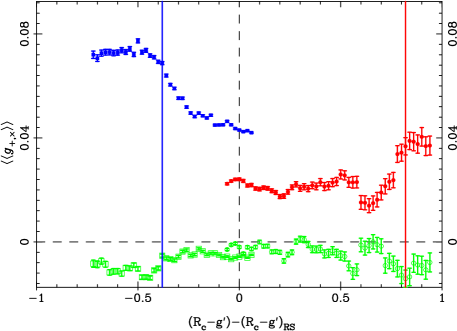
Figure 3.— Mean distortion strength $\langle\langle g_{+,\times}\rangle\rangle$ over the radii of $1^{\prime}\leq r\leq 18^{\prime}$, as a function of color. The background samples are defined with galaxies redder or bluer than the red-sequence by at least the color offsets given by the $x$-label. The distortion strength is changed due to dilution by cluster members. The red circle and blue square points denote the mean tangential distortion $\langle\langle g_{+}\rangle\rangle$ for redder and bluer background samples, respectively. The green circle and square points denote the mean tangential distortion for the $45$ degree rotated component $\langle\langle g_{\times}\rangle\rangle$ for redder and bluer samples, respectively. The two vertical solid lines denote our choices of the color cuts used to define the red/blue background galaxy samples shown in Figure 4. The details are described in Umetsu & Broadhurst (2008) and Okabe et al. (2010b).

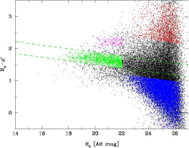
Figure 4.— Color-magnitude diagram. Green points are member galaxies of which spatial distribution is shown in the top right and bottom left panels of Figure 6. Two green dashed lines represent the width of the red sequence. The red and blue points are the background galaxy samples, used for the lensing distortion analysis, whose colors are redder and blue than the red sequence, respectively. The magenta points denote a sample of galaxies in the right bottom panel of Figure 6.

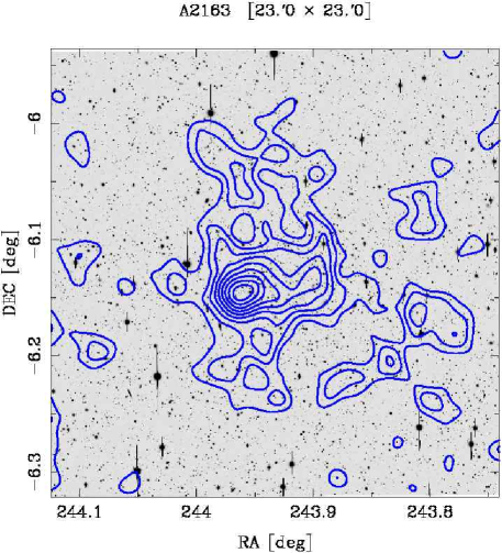
Figure 5.— Subaru $R_{\rm c}$-band image ($23\farcm\times 23\farcm$) overlaid with contours of the $\kappa$-field reconstructed from the weak-shear field, in units of $1\sigma$ reconstruction error $\delta\kappa=0.0404$.

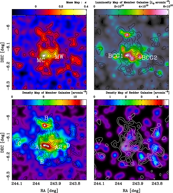
Figure 6.— Top left: reconstructed lensing $\kappa$-field in units of $1\sigma$ reconstruction error. The bimodal structure in the central region is clearly found. The significance levels of bimodal peaks are $\sim 10\sigma$ and $\sim 5.6\sigma$, which are referred to as MC and MW, respectively. Top right : luminosity map for red-sequence galaxies in the $R_{\rm c}$ band. Overlaid are the contours of the $\kappa$ field. Two crosses denote BCG positions. Bottom left : density map for red-sequence galaxies in units of arcmin^-2. The four density clumps other than the bimodal structure, discovered by M08 (Maurogordato et al., 2008), are confirmed. All labels for the density clump are quoted from M08. Bottom right : density map for galaxies whose color is redder by $\sim 0.6$ at $R_{\rm c}=22~{}{\rm ABmag}$ than those of member galaxies.

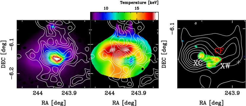
Figure 7.— Left: adaptively-smoothed Chandra X-ray image ($14\farcm\times 14\farcm$) in the $0.5-2.5$ keV band. Overlaid are the contours of the lensing $\kappa$-field in units of $1\sigma$ reconstruction error (Figure 6). Middle : temperature map from XMM-Newton data with the same mass contours as those in the left panel. Right: high resolution residual Chandra image obtained after subtracting large scales of the denoised wavelet transform of the X-ray image. Two components (XC and XW) are clearly found in the X-ray emitting core. Two crosses denote BCG positions. Red (color version) or dark gray (black and white version) curved line represents the cold front (CF; see B11). Overlaid are the same mass contours above the $3\sigma$ significance. The offsets between the X-ray core and two mass peaks are clearly found.

Figure 8.— Profiles of the tangential shear component (top panel), $g_{+}$, and the $45$ degree rotated component (bottom panel), $g_{\times}$. The solid and dashed lines are the best-fit NFW and SIS models, respectively. The SIS model is strongly disfavored ($\sim 5\sigma$ level) for a cluster mass profile.

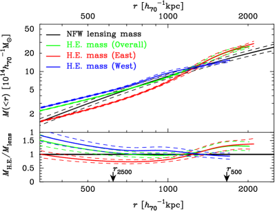
Figure 9.— Comparison of NFW lensing mass and hydrostatic masses. Black color represents the NFW lensing mass profile. Green, red and blue colors represent the hydrostatic mass in overall, east and west sectors (B11; Bourdin et al., 2011), respectively. The solid and dashed lines are the best fit values and the 68% CL uncertainty errors, respectively. The arrows denote the overdensity radii $r_{2500}$ and $r_{500}$ determined by weak-lensing analysis. We use $h_{70}=H_{0}/70\;\rm{km\;s^{-1}\;Mpc^{-1}}=1.0$.

Figure 10.— Ram pressure stripping condition of the subcluster core. $A$ is a fudge factor associated with hydrodynamical instabilities or gas heating. The vertical line denotes the gradient of the line-of-sight velocity (M08). The arrow denotes an order of the infall velocity (Equation (15)) expected from masses for main and sub clusters, measured by two-dimensional weak-lensing analysis.

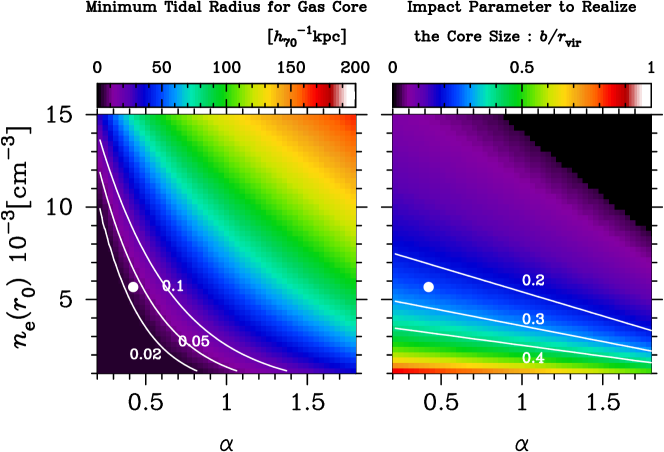
Figure 11.— Left : minimum tidal radius in the parameter plane of core density normalization, $n_{e}(r_{0})=n_{e,0}$ at the cold front $r=r_{0}$ and slope $\alpha$. The contours represent tidally truncated core sizes of $0\farcm 02,0\farcm 05$, and $0\farcm 1$ in units of arcmin. The point denotes the observed parameters for the core XW. Right: impact parameter to realize the observed core size. The contours are $(0.2-0.4)r_{\rm vir}$. The point is the same as that in the left panel.

Table 1Optical subclumps

Names	$L_{\rm R_{c}}(<2\farcm)$	S/N
(1)	(2)	(3)
C	$1.47$	$2.0$
D	$0.94$	$1.7$
E	$2.38$	$2.7$

Table 2Best-fit Mass Profile Parameters

Method	$M_{\rm vir}$	$c_{\rm vir}$	$M_{200}$	$c_{200}$	$M_{500}$	$c_{500}$
	$(10^{14}h^{-1}M_{\odot})$		$(10^{14}h^{-1}M_{\odot})$		$(10^{14}h^{-1}M_{\odot})$
(1)	(2)	(3)	(4)	(5)	(6)	(7)
1D WL	$24.24_{-4.55}^{+6.00}$	$2.84_{-0.61}^{+0.71}$	$18.86_{-3.17}^{+3.99}$	$2.18_{-0.50}^{+0.57}$	$11.18_{-1.46}^{+1.64}$	$1.35_{-0.33}^{+0.39}$
2D WL	$26.72_{-5.79}^{+4.72}$	$2.58_{-0.59}^{+0.48}$	$20.32_{-4.08}^{+3.21}$	$1.99_{-0.49}^{+0.39}$	$11.13_{-1.55}^{+1.31}$	$1.37_{-0.30}^{+0.20}$
Dynamics (M08)	–	–	$27.3\pm 2.8$	–	–	–
X-ray (B11) : H.E.	–	–	–	–	$17.29^{+0.35}_{-0.63}$	–
X-ray : H.E. west	–	–	–	–	$10.15^{+0.42}_{+0.21}$	–
X-ray : H.E. east	–	–	–	–	$18.55^{+1.33}_{-0.84}$	–
WL (Radovich et al. 2008)	$15.4\pm 2.8$	–	$12.6\pm 2.1$	–	$8.4\pm 1.4$	–

Table 3Multi-component Analysis of the Two-dimensional Shear Pattern

Parameters	NFW+TSIS	NFW+TSIS+NFW	NFW+TSIS+TSIS
(1)	(2)	(3)	(4)
$M_{\rm vir,main}$	$20.98_{-7.38}^{+4.67}\times 10^{14}h^{-1}M_{\odot}$	$16.46_{-5.90}^{+3.69}\times 10^{14}h^{-1}M_{\odot}$	$18.79_{-6.68}^{+4.31}\times 10^{14}h^{-1}M_{\odot}$
$c_{\rm vir,main}$	$2.88_{-0.82}^{+0.70}$	$3.44_{-1.05}^{+0.78}$	$3.14_{-0.96}^{+0.74}$
$M_{\rm MW}$	$2.13_{-0.85}^{+0.95}\times 10^{14}h^{-1}M_{\odot}$	$2.08_{-0.97}^{+0.96}\times 10^{14}h^{-1}M_{\odot}$	$2.09_{-0.96}^{+0.96}\times 10^{14}h^{-1}M_{\odot}$
$r_{t,{\rm MW}}$	$1.39_{-0.38}^{+0.47}h^{-1}{\rm Mpc}$	$1.35_{-0.41}^{+0.49}h^{-1}{\rm Mpc}$	$1.37_{-0.39}^{+0.48}h^{-1}{\rm Mpc}$
$M_{\rm B}$	–	$2.43_{-1.15}^{+0.90}\times 10^{14}h^{-1}M_{\odot}$	$1.44_{-0.84}^{+0.64}\times 10^{14}h^{-1}M_{\odot}$
($\alpha$, $\delta$)c,main	($243.958_{-0.002}^{+0.003}$, $-6.147_{-0.003}^{+0.003}$)	($243.958_{-0.003}^{+0.003}$, $-6.146_{-0.003}^{+0.003}$)	($243.958_{-0.003}^{+0.004}$, $-6.147_{-0.003}^{+0.003}$)
($\alpha$, $\delta$)c,MW	($243.905_{-0.005}^{+0.008}$, $-6.125_{-0.005}^{+0.007}$)	($243.905_{-0.005}^{+0.009}$, $-6.125_{-0.005}^{+0.007}$)	($243.905_{-0.005}^{+0.009}$, $-6.125_{-0.005}^{+0.008}$)
($\alpha$, $\delta$)c,B	–	($243.969_{-0.005}^{+0.009}$, $-6.042_{-0.005}^{+0.005}$)	($243.968_{-0.005}^{+0.007}$, $-6.042_{-0.006}^{+0.003}$)

References

- Arnaud et al. (1992) Arnaud, M. et al.,1992, ApJ, 390, 345.
- Arnaud et al. (2010) Arnaud, M., Pratt, G. W., Piffaretti, R., Böhringer, H., Croston, J., H., & Pointecouteau, E., 2010, A&A,517,A92.
- Bardeau et al. (2007) Bardeau, S., Soucail, G., Kneib, J.-P., Czoske, O., Ebeling, H., Hudelot, P., Smail, I., & Smith, G. P.,2007, A&A, 470, 449.
- Bartelmann & Schneider (2001) Bartelmann, M., Schneider, P., 2001, Phys. Rep., 340, 219.
- Becker & Kravtsov (2010) Becker, M. R. & Kravtsov, A. V., 2010, ApJ submitted (arXiv:1011.1681).
- Binney & Mamon (1982) Binney, J., & Mamon, G., A.,1982,MNRAS,200,361.
- Bourdin et al. (2011) Bourdin, H., Arnaud, M., Mazzotta, P., Pratt, G. W., Sauvageot, J.-L., Martino, R., Maurogordato, S., Cappi, A., Ferrari, C., Benoist, C., 2011, A&A 527, A21. (B11)
- Broadhurst et al. (2005) Broadhurst, T., Takada, M., Umetsu, K., et al., 2005, ApJL, 619, 143. K. & Setti, G., 2009,A&A,507,661.
- Clowe et al. (2006) Clowe, D., et al. 2006, A&A, 451, 395
- Cypriano et al. (2004) Cypriano, E. S., Sodré, L., Jr., Kneib, J.-P., & Campusano, L. E. 2004, ApJ, 613, 95
- Duffy et al. (2008) Duffy, A., R., Schaye, J., Kay, S., T. & Dalla V., C., 2008,MNRAS,390,L64.
- Erben et al. (2001) Erben, T., van Waerbeke, L., Bertin, E., Mellier, Y., & Schneider, P. 2001, A&A, 366, 717.
- Elbaz et al. (1995) Elbaz, D., Arnaud, M., Boehringer, H.,1995, A&A,293, 337.
- Feretti et al. (2001) Feretti, L., Fusco-Femiano, R., Giovannini, G. & Govoni, F.,2001,A&A, 373, 106.
- Feretti et al. (2004) Feretti, L., Orrù, E., Brunetti, G., Giovannini, G., Kassim, N. & Setti, G. 2004, A&A,423,111.
- Gray et al. (2002) Gray, M. E., Taylor, A. N., Meisenheimer, K., Dye, S., Wolf, C. & Thommes, E.,2002, ApJ,568,141.
- Gavazzi et al. (2003) Gavazzi, R., Fort, B., Mellier, Y., Pelló, R., Dantel-Fort, M., 2003, A&A, 403, 11
- Hernquist (1990) Hernquist, L.,1990, ApJ,356, 359.
- Hoekstra (2007) Hoekstra, H., 2007,MNRAS,379, 317.
- Ilbert et al. (2009) Ilbert, O., et al. 2009, ApJ, 690, 1236.
- Kaiser & Squires (1993) Kaiser, N. & Squires, G. 1993, ApJ, 404, 441.
- Kaiser et al. (1995) Kaiser, N., Squires, G., Broadhurst, T., 1995, ApJ, 449, 460.
- Kawaharada et al. (2010) Kawaharada, M., Okabe,N., Umetsu, K., Takizawa, M., Matsushita, K., Fukazawa, Y. Hamana, T., Miyazaki, S., Nakazawa, K., & Ohashi, T., 2010,ApJ,714, 423.
- Kravtsov et al. (2006) Kravtsov, A., V., Vikhlinin, A., A., & Nagai, D., 2006,ApJ,650,128.
- La Barbera et al. (2004) La Barbera, F., Merluzzi, P., Busarello, G., Massarotti, M. & Mercurio, A. 2004, A&A,425, 797.
- Łokas & Mamon (2001) Łokas, E. L. & Mamon, G., A., 2001, MNRAS,321,155.
- Mahdavi et al. (2007) Mahdavi, A., Hoekstra, H., Babul, A., Balam, D., D., & Capak, P., L., 2007,ApJ,668,806.
- Mahdavi et al. (2008) Mahdavi, A., Hoekstra, H.; Babul, A., Henry, J. P., 2008, MNRAS,384,1567
- Markevitch & Vikhlinin (2001) Markevitch, M. & Vikhlinin, A., 2001,ApJ,563,95.
- Markevitch & Vikhlinin (2007) Markevitch, M. & Vikhlinin, A., 2007, PhR,443,1.
- Maurogordato et al. (2008) Maurogordato, S., Cappi, A., Ferrari, C., Benoist, C., Mars, G., Soucail, G., Arnaud, M., Pratt, G. W., Bourdin, H.& Sauvageot, J.-L., 2008, A&A, 481, 593 (M08).
- Mazzotta et al. (2004) Mazzotta, P., Rasia, E., Moscardini, L., & Tormen, G. 2004, MNRAS, 354, 10.
- Meneghetti et al. (2010) Meneghetti, M., Rasia, E., Merten, J., Bellagamba, F., Ettori, S., Mazzotta, P., Dolag, K. & Marri, S., 2010, A&A, 514, A93.
- Merten et al. (2011) Merten, J. et al., 2011, MNRAS accepted (arXiv:1103.2772)
- Navarro, Frenk, & White (1996) Navarro, J. F.,Frenk, C. S. & White, S. D. M. 1996, ApJ, 462, 563.
- Nord et al. (2009) Nord, M., et al. 2009, A&A, 506, 623
- Planck Collaboration (2011) Planck Collaboration : Ade, P., A., R.,, Aghanim, N., Arnaud, M. et al. 2011, arXiv:1101.2026
- Oguri et al. (2010) Oguri, M., Takada, M., Okabe, N., & Smith, G., P., 2010, MNRAS, 405,2215.
- Okabe & Umetsu (2008) Okabe, N. & Umetsu, K. 2008, PASJ, 60, 345
- Okabe et al. (2010a) Okabe, N., Okura, Y., & Futamase, T., 2010, ApJ, 713, 291.
- Okabe et al. (2010b) Okabe, N., Takada, M., Umetsu, K., Futamase, T. & Smith, G., P., 2010, PASJ, 62, 811.
- Okabe et al. (2010c) Okabe, N., Zhang, Y.,-Y., Finoguenov, A.,; Takada, M., Smith, G., P., Umetsu, K., & Futamase, T., 2010, ApJ, 721, 875.
- Ouchi et al. (2004) Ouchi, M., et al. 2004, ApJ, 611, 660.
- Radovich et al. (2008) Radovich, M., Puddu, E., Romano, A., Grado, A. & Getman, F., 2008, A&A,487, 55.
- Ricker & Sarazin (2001) Ricker, P. M. & Sarazin, C. L. 2001, ApJ, 561, 621.
- Schneider (2006) Schneider, P., “Weak Gravitational Lensing”, Lecture Notes of the 33rd Saas-Fee Advanced Course, G. Meylan, P. Jetzer & P. North (eds.), Springer-Verlag: Berlin, p.273
- Shan et al. (2010) Shan, H., Qin, B., Fort, B., Tao, C., Wu, X.-P., & Zhao, H. 2010, MNRAS, 406, 1134
- Stanek et al. (2010) Stanek, R., Rasia, E., Evrard, A., E., Pearce, F., & Gazzola, L., 2010, ApJ,715,1508.
- Tormen et al. (1998) Tormen, G., Diaferio, A., & Syer, D., 1998,MNRAS, 299, 728.
- Tormen et al. (2004) Tormen, G., Moscardini, L. & Yoshida, N., 2004, MNRAS, 350, 1397.
- Takizawa (2006) Takizawa, M., 2006, PASJ, 58, 925.
- Umetsu & Broadhurst (2008) Umetsu, K. & Broadhurst, T., 2008, ApJ, 684, 177.
- Umetsu et al. (2009) Umetsu, K. et al. 2009, ApJ, 694, 1643.
- Umetsu et al. (2010) Umetsu, K. et al. 2010. ApJ, 714, 1470.
- Vikhlinin et al. (2009a) Vikhlinin, A., Burenin, R. A., Ebeling, H., Forman, W. R., Hornstrup, A., Jones, C., Kravtsov, A. V., Murray, S. S., Nagai, D., Quintana, H., & Voevodkin, A. 2009a, ApJ, 692, 1033.
- Vikhlinin et al. (2009b) Vikhlinin, A., Kravtsov, A. V., Burenin, R. A., Ebeling, H., Forman, W. R., Hornstrup, A., Jones, C., Murray, S. S., Nagai, D., Quintana, H., Voevodkin, A., 2009b,ApJ,692,1060.
- Watanabe et al. (2011) Watanabe, E.,Takizawa, M., Nakazawa, K., Okabe, N., Kawaharada, M., Babul, A., Finoguenov,A., Smith, G., P., & Taylor, J., 2011, PASJ, 63, 357.
- Zhang et al. (2008) Zhang, Y.-Y., Finoguenov, A., Böhringer, et al. 2008, A&A, 482, 451.
- Zhang et al. (2010) Zhang, Y.-Y., Okabe, N., Finoguenov, A., et al. 2010, ApJ, 711, 1033