Bose-Einstein condensation transition studies for atoms confined in Laguerre-Gaussian laser modes

Abstract

Multiply-connected traps for cold, neutral atoms fix vortex cores of quantum gases. Laguerre-Gaussian laser modes are ideal for such traps due to their phase stability. We report theoretical calculations of the Bose-Einstein condensation transition properties and thermal characteristics of neutral atoms trapped in multiply connected geometries formed by Laguerre-Gaussian (LG${}_{p}^{l}$) beams. Specifically, we consider atoms confined to the anti-node of a LG${}_{0}^{1}$ laser mode detuned to the red of an atomic resonance frequency, and those confined in the node of a blue-detuned LG${}_{1}^{1}$ beam. We compare the results of using the full potential to those approximating the potential minimum with a simple harmonic oscillator potential. We find that deviations between calculations of the full potential and the simple harmonic oscillator can be up to $3\%-8\%$ for trap parameters consistent with typical experiments.

Bose-Einstein condensation (BEC) has led to a wealth of new physics, from applications in inertial measurements to fundamental studies of statistical mechanical phenomena and superfluidity dg99 . Among the first experiments probing BEC were those that explored the thermal properties and transition characteristics, with particular emphasis on the effect of trap geometry mav96 ; ejm96 . An important avenue of investigation in the connection between condensed matter (super-fluidity) and BEC l38 of atomic gases is the experimental mah99 ; mcw00 ; arv01 and the theoretical dcl98 ; cj09 studies of vortices. It was recognized early that a trap potential with the ability to pin a vortex core would be an advance in the study and application of these quantized rotations in BEC rac07 . Toward this end, researchers have developed novel multiply-connected trap geometries. A toroidal potential locally fixes a vortex state, thus encouraging rotational stability for more precise measurements and may help facilitate the development of devices utilizing vortices, such as the atomic squid detector adw03 and the ultra-stable gyroscope tkd09 . Recent progress in toroidal potentials has been seen in the confinement of cold atoms bsc01 , BEC orv00 ; ar02 , and creation of vortex states rac07 .
An important method for creating toroidal geometries uses higher-order Laguerre-Gaussian laser modes. The Laguerre-Gaussian beams, as a set of solutions to Maxwell’s equations abs92 , represent stable modes of laser propagation. The radial electric field is proportional to an associated Laguerre polynomial, $L_{p}^{l}$, and a Gaussian function. The electric field of LG${}_{p}^{l}$ laser modes has an azimuthal winding phase given by $e^{-il\phi}$ abs92 , and the $p+1$ radial intensity nodes provide a variety of multiply connected geometries for vortex studies. LG${}_{p}^{l}$ photons have a quantized orbital angular momentum (OAM) of $l\hbar$ per photon. This property can also be exploited to create vortices through the coupling of photon-matter OAM, as proposed by mzw97 ; kwm07 and demonstrated by rac07 ; wlb08 .
We explore the thermal properties (the transition temperature, the population of atoms in the ground state, and the specific heat) of a Bose gas trapped in a LG${}_{p}^{l}$ dipole trap, utilizing the complete LG${}_{p}^{l}$ potential. These results are compared to those where the confining potential minimum has been approximated as a simple harmonic oscillator. Previously, the simple harmonic oscillator approximation has been used in calculations to determine the ground state energies, density profiles, and the transition temperature in LG beams spr99 ; wad00 ; tw01 .
Consider an atom in an inhomogeneous laser field whose angular frequency, $\omega$, is near enough to a resonant angular frequency, $\omega_{0}$, that the coupling between any other pair of states can be ignored. The laser detuning, $\Delta=\omega-\omega_{0}$, is sufficiently large that the probability of photon absorption is negligible. The atom experiences an attractive force toward regions of high laser intensity when the detuning is negative ($\Delta<0$) and a repulsive force away from regions of high laser intensity when the detuning is positive ($\Delta>0$).
We investigate two physically realizable toroidal trapping geometries formed by the lowest two orders in a LG${}_{p}^{l}$ beam (with non-zero angular momentum): the LG${}_{0}^{1}$ red-detuned trap and the LG${}_{1}^{1}$ blue-detuned trap. The intensity profile for the LG${}_{0}^{1}$ mode is given in Figure 1 (a). For $\Delta<0$, this shape satisfies the desired toroidal geometry with atoms confined to regions of high laser intensity. Blue detuned dipole traps are preferred for applications where external perturbation needs to be minimized. Atoms spend the majority of their time in regions of lowest intensity. The LG${}_{1}^{1}$ beam satisfies this condition, and a sample profile is shown in Figure 1 (b).

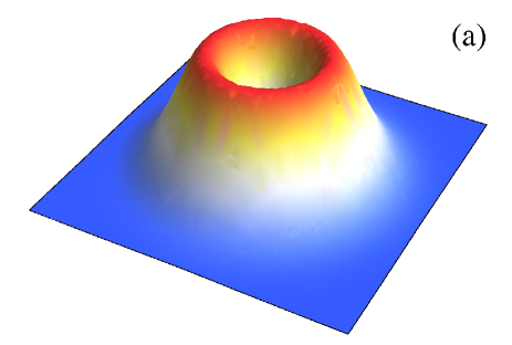
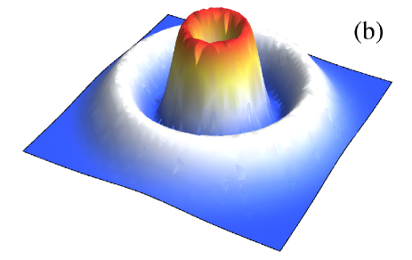
Figure 1: (Color online) The transverse intensity profile for (a) the LG${}_{0}^{1}$ mode and (b) the LG${}_{1}^{1}$ mode.

The potential energy of an atom in the presence of a LG${}_{p}^{l}$ mode is given by wad00 ,

$$U_{p}^{l}=\frac{\hbar\Gamma^{2}}{8I_{sat}\Delta}\frac{2p!}{p+l}\frac{P_{0}}{\pi w^{2}}\left(\frac{2r^{2}}{w^{2}}\right)^{l}\left[L_{p}^{l}\left(\frac{2r^{2}}{w^{2}}\right)\right]^{2}e^{-2r^{2}/w^{2}},$$ (1)

where $P_{0}$ is the total laser power, $\Gamma=2\pi\times 6.1$ MHz is the natural line width for ⁸⁷Rb, and $w$ is the beam waist. The resonant saturation intensity is $I_{sat}=\pi hc/3\lambda^{3}\tau$, where $\lambda$ is the resonance wavelength and $\tau$ is the lifetime of the resonant state. We work in cylindrical coordinates where the dipole potential only confines in the transverse $r$-dimension. To confine along the direction of laser propagation ($z$-dimension), we will assume a harmonic potential. One dimensional confinement can be constructed via an anisotropic magnetic trap whose trapping potential in the radial dimension is small enough to be ignored compared to the laser potential pae95 ; gvl01 . With the inclusion of the 1-D harmonic confinement together with the radial dipole potential in Equation (1), the confining potential for both laser modes has the form,

$$\begin{array}[]{lll}U_{0}^{1}&=&2V\left(\frac{2r^{2}}{w^{2}}\right)e^{-2r^{2}/w^{2}}+\frac{1}{2}m\omega^{2}_{z}z^{2}\\ U_{1}^{1}&=&V\left(\frac{2r^{2}}{w^{2}}\right)\left(2-\frac{2r^{2}}{w^{2}}\right)^{2}e^{-2r^{2}/w^{2}}+\frac{1}{2}m\omega^{2}_{z}z^{2},\end{array}$$ (4)

where $\omega_{z}$ is the trapping frequency in the $z$-direction and $m$ is the mass of the confined atom. The constant $V$ is the product of three physical quantities,

$$V=\frac{\hbar\Gamma}{8}\frac{I_{0}}{I_{sat}}\frac{\Gamma}{\Delta}.$$

The first factor is an energy scale set by the energy width of the excited state. The second factor is the ratio of an intensity term ($I_{0}=P_{0}/\pi w^{2}$) to the saturation intensity. The last factor is a ratio of the line width to the laser detuning. These factors combine to set the scale of the trap strength.
The 1-D radial cross-section of both potentials in Equation (4) are plotted in Figure 2. The calculations are done in dimensionless units. All the lengths are scaled by $a_{ho}=\sqrt{\hbar/m\omega_{z}}$, the harmonic oscillator length of the simple harmonic confining potential in the $z$-direction. All the energies are scaled by $\epsilon_{ho}=\hbar\omega_{z}/2$, the energy of the corresponding 1-D ground state in the $z$-direction. Dimensionless quantities are identified with a tilde ($\sim$) set above the term: $\tilde{r}=r/a_{ho}$, $\tilde{z}=z/a_{ho}$, $\tilde{w}=w/a_{ho}$, $\tilde{\epsilon}=\epsilon/\epsilon_{ho}$, and $\tilde{v}=V/\epsilon_{ho}$. Making these substitutions into the potentials, Equation (4) becomes,

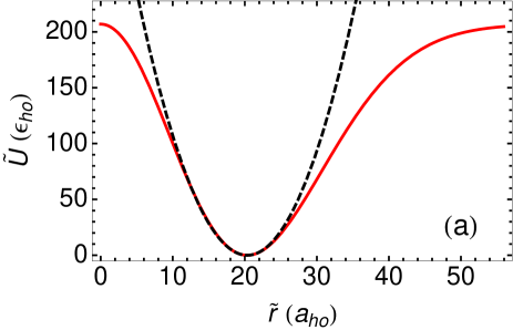
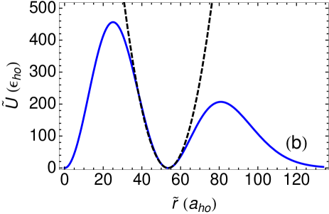
Figure 2: (Color online) The radial potential energy (in units of $\epsilon_{ho}$) of an atom in specific LG${}_{p}^{l}$ laser modes as a function of distance from the center of the laser beam (in units of $a_{ho}$). In both plots, the solid line corresponds to the full LG${}_{p}^{l}$ dipole potential, and the dashed line represents the second order expansion about the minima of the potential (SHO approximation).

$$\begin{array}[]{lll}\tilde{U}_{0}^{1}&=&-4\frac{\tilde{v}}{\tilde{w}^{2}}\tilde{r}^{2}e^{-2\tilde{r}^{2}/\tilde{w}^{2}}+\tilde{z}^{2}\\ \tilde{U}_{1}^{1}&=&8\frac{\tilde{v}}{\tilde{w}^{6}}\tilde{r}^{2}\left(\tilde{w}^{2}-\tilde{r}^{2}\right)^{2}e^{-2\tilde{r}^{2}/\tilde{w}^{2}}+\tilde{z}^{2}.\end{array}$$ (7)

We explore a few of the thermal properties of a cold Bose gas confined in a toroidal potential. One such property is the BEC transition temperature, $T_{c}$. We calculate $T_{c}$ following the procedure outlined in bpk87 . In the limit when $N\rightarrow\infty$ and $k_{B}T$ is much larger than the energy spacing of the confining potential, then

$$N=N_{0}+\int^{\infty}_{0}\rho(\epsilon)n(\epsilon)d\epsilon,$$ (8)

where $N_{0}$ is the number of atoms in the ground state, $\rho(\epsilon)$ is the density of states, and $n(\epsilon)$ is the usual Bose distribution occupation number $1/(e^{\beta(\epsilon-\mu)}-1)$, where $\beta=1/k_{B}T$ and $\mu$ is the chemical potential. The density of states is

$$\rho(\epsilon)=\frac{(2m)^{3/2}}{(2\pi)^{2}\hbar^{3}}\int_{V^{*}(\epsilon)}\sqrt{\epsilon-U(\textbf{r})}d\textbf{r},$$ (9)

where $V^{*}(\epsilon)$ is the classical spatial volume spanned by a particle with energy $\epsilon$.
As the phase space of the system decreases, the ground state population remains unoccupied until the chemical potential approaches zero. Thus, the transition temperature, $T_{c}$, can be found by setting $\mu=0$ and $N_{0}=0$. The heat capacity, $C(T)$, is piecewise continuous, but a discontinuity at $T_{c}$ is a signature of the BEC phase transition. The heat capacity is $C(T)=\partial E(T)/\partial T$ where the total energy of the system is

$$E(T)=\int^{\infty}_{0}\epsilon\rho(\epsilon)n(\epsilon)d\epsilon.$$ (10)

Equations (8) through (10) can be solved analytically when the potential is expanded up to the second order about the potential minimum. This is the simple harmonic oscillation (SHO) approximation used in spr99 ; wad00 ; tw01 . For our system and notation, the confining potentials are given by

$$\begin{array}[]{lll}(\tilde{U}_{0}^{1})_{ho}&=&\frac{8\tilde{v}}{e\tilde{w}^{2}}\left(\tilde{r}-\frac{\tilde{w}}{\sqrt{2}}\right)^{2}+\tilde{z}^{2}\\ (\tilde{U}_{1}^{1})_{ho}&=&\frac{32\tilde{v}}{e^{2}\tilde{w}^{2}}\left(\tilde{r}-\tilde{w}\right)^{2}+\tilde{z}^{2},\end{array}$$ (13)

in the SHO approximation. Defining $(\tilde{\rho}_{p}^{l})_{ho}\equiv\rho\epsilon_{ho}$ for a specific LG${}_{p}^{l}$ potential, the densities of states are

$$\begin{array}[]{lll}(\tilde{\rho}_{0}^{1})_{ho}(\tilde{\epsilon})&=&\sqrt{\frac{e}{\tilde{v}}}\frac{\tilde{w}^{2}}{12}\tilde{\epsilon}^{3/2}\\ (\tilde{\rho}_{1}^{1})_{ho}(\tilde{\epsilon})&=&\sqrt{\frac{e^{2}}{2\tilde{v}}}\frac{\tilde{w}^{2}}{12}\tilde{\epsilon}^{3/2}.\end{array}$$ (16)

From here, we carry out the integrations in Equation (8) to find the BEC transition temperature, $(T_{p}^{l})_{ho}$,

$$\begin{array}[]{lll}(T_{0}^{1})_{c}&=&4\left(\frac{\tilde{v}}{4\pi e}\right)^{1/5}\left(\frac{N}{\tilde{w}^{2}\zeta(5/2)}\right)^{2/5}\frac{\epsilon_{ho}}{k_{B}}\\ (T_{1}^{1})_{c}&=&4\left(\frac{\tilde{v}}{2\pi e^{2}}\right)^{1/5}\left(\frac{N}{\tilde{w}^{2}\zeta(5/2)}\right)^{2/5}\frac{\epsilon_{ho}}{k_{B}},\end{array}$$ (19)

where the term $\zeta(5/2)$ is the Riemann Zeta function.
Calculation of $T_{c}$ using the full potential given by Equation (7) must be done numerically. For a given $\tilde{w}$ and $\tilde{v}$, the density of states (Equation (9)) is numerically integrated for a discrete set of energies, $\epsilon_{i}$. The numerical integration is done in Mathematica mathematica  and we provide our source code online lgnotebook . Twenty values of the density of states are calculated covering an energy range $\epsilon_{i}=0$ to $\epsilon_{max}$. The value of $\epsilon_{max}$ is determined such that most of the Bose-Einstein distribution is accounted for, while being certain that the energy range sufficiently maps out the most probable portions of the trap occupied by the particle. To do this, we find the location of the critical temperature of the SHO approximation with respect to the potential barrier of the corresponding LG${}_{p}^{l}$ mode. The energy range is adjusted to span this region. The limits of integration for Equation (9) are determined by solving Equation (7) for the classical volume accessible by a particle of energy $\epsilon_{i}$. For the radial classical turning points, we use the Newton-Raphson numerical technique. The resulting set of points of the density of states, $\rho_{i}(\epsilon_{i})$, are fit to the analytical expression,

$$\rho(\epsilon)=\sigma\epsilon^{\eta},$$ (20)

where the factors $\sigma$ and $\eta$ are the fitting parameters. This model has a general form that is characteristic for many systems. For example, a Bose gas with no external potential results in $\eta=1/2$, one confined by a 3-D isotropic oscillator gives $\eta=2$, and both harmonic approximations to the LG beams given in Equations (13) and (16) result in $\eta=3/2$. We substitute the fitted function into Equation (8) and analytically integrate to find $T_{c}$ for a given $N$ (in our case, we choose a value of $N=10^{6}$). Finally, we analytically integrate Equation (10) to find the total energy, $E(T)$, and then the heat capacity.

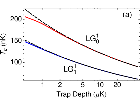
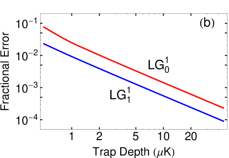
Figure 3: (Color online) (a) $T_{c}$ calculations using both the full potential (solid curve) and the SHO approximation (dashed curve) as a function of trap depth, where the radial trap frequency is held equal to the axial trap frequency, $\omega_{z}/2\pi=100\textrm{Hz}$. (b) The factional error of the SHO calculation.

Figures 3 through 7 show the expected BEC transition temperature, ground state fraction, and heat capacity for a ⁸⁷Rb gas confined in the LG${}_{p}^{l}$ modes. We also show the corresponding harmonic approximations and compare with the exact calculation for different laser beam parameters. Figure 3 shows $T_{c}$ in the LG${}_{0}^{1}$ (upper line) and the LG${}_{1}^{1}$ (lower line) modes as a function of the trap depth while maintaining equal trap frequencies in the axial and radial directions. The trap depth is the height of the lowest confining barrier of the radial potential (Figure 2). The axial trap frequency is set to $\omega_{z}/2\pi=100$ Hz, typical of magnetic trap experiments dg99 . The trap depth is changed by adjusting $\tilde{v}$, equivalent to adjusting the power or detuning of the trapping laser. At the same time, $\tilde{w}$ is adjusted so the radial trap frequency is maintained at $\omega_{r}=\omega_{z}$. The critical temperature is calculated using the full potential (solid line) and using the SHO approximation of the potential well (dotted line). Note that $T_{c}$ decreases with the trap depth in this figure because of the constraint $\omega_{r}=\omega_{z}$. As the laser power increases, the beam waist must increase to maintain constant $\omega_{r}$. This increases the trap volume, and decreases $T_{c}$. Figure 3 (b) shows the fractional error of the SHO approximations compared to the exact calculation. The uncertainty is largest when the transition temperature approaches the trap depth. The classical volume accessed by particles includes a larger fraction of the potential well where the harmonic approximation is no longer valid. We calculate fractional differences from $7.6\%$ to $0.023\%$ over a trap depth of $0.1~{}\mu\textrm{K}$ to $10~{}\mu\textrm{K}$.

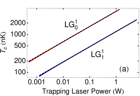
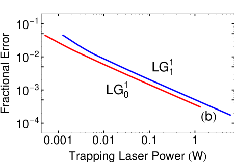
Figure 4: (Color online) (a) $T_{c}$ as a function of the laser power. The beam parameters are $w_{r}=50~{}\mu\textrm{m}$ and $\Delta/2\pi=1000$ GHz. The comparison is made using both the full potential (solid curve) and the SHO approximation (dashed curve) while keeping the trapping beam waist fixed and simultaneously increasing the laser power. In addition, the axial harmonic trapping frequency is adjusted such that the trap remains symmetric at all laser powers. (b) The fractional error of the SHO calculation.

In contrast to Figure 3, Figure 4 considers a symmetric case where the beam waist is held constant while increasing the trap depth. This corresponds to the trap volume decreasing as the trap depth increases. The critical temperature in the LG${}_{0}^{1}$ (upper line) mode and the LG${}_{1}^{1}$ (lower line) mode is plotted as a function of the laser power. We fix the beam waist at $w=42~{}\mu\textrm{m}$  for the LG${}_{0}^{1}$ mode, and $w=58~{}\mu\textrm{m}$ for the LG${}_{1}^{1}$ mode. The laser detuning is set to $|\Delta|/2\pi=1000$ GHz for both modes. The laser power is varied over a range of $0.52~{}\textrm{mW}-1.3~{}\textrm{W}$ for the LG${}_{0}^{1}$ mode, and $1.3~{}\textrm{mW}-5.9~{}\textrm{W}$. This has the effect of increasing the trap depth and $\omega_{r}$. To keep the trap symmetric, we allow $\omega_{z}$ to change such that $\omega_{z}=\omega_{r}$. An increase in the trap depth has an effect of increasing $T_{c}$. For this case, we also make the SHO approximation to the confining potential. The fractional differences are from $4.5\%$ to $0.017\%$. Like in Figure 3, the largest error occurs when the trap depth and the transition temperature are comparable. As a larger fraction of the particles populate larger regions of the potential, the particles occupy regions where the potential becomes less harmonic. We replace the constant, $\sigma$ in Equation (20), with the polynomial $\sigma(\epsilon)=\sigma_{0}+\sigma_{1}\epsilon+\sigma_{2}\epsilon^{2}\cdots$, where the minimum number of terms were kept such that the result converged.

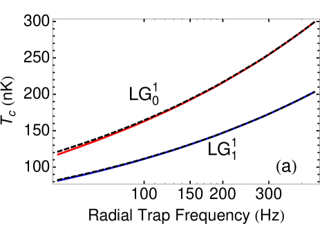
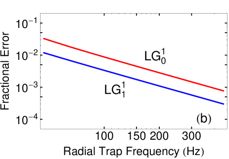
Figure 5: (Color online) (a) $T_{c}$ calculations using both the full potential (solid curve) and the SHO approximation (dashed curve) while keeping the trapping beam waist fixed and simultaneously increasing the laser power. Thus, the effects of adjusting the radial trapping frequency with respect to the axial frequency. Again, the axial frequency is fixed at $100\textrm{Hz}$. (b) The factional error of the SHO calculation.

Figure 5 considers the effect on $T_{c}$ when the trapping frequencies in the two trapping dimensions ($r$ and $z$) are allowed to vary with respect to each other. The symmetric case ($\omega_{r}/2\pi=100$ Hz on the horizontal axis in Figure 5) corresponds to a laser power of $P_{0}=10$ mW, a beam waist $w=50~{}\mu\textrm{m}$, and a detuning of $|\Delta|/2\pi=1000$ GHz. These values are concurrent with typical harmonic oscillator lengths of $a_{ho}=1~{}\mu\textrm{m}$ reported by dg99 . We vary the radial trap frequency by fixing the waist of the trapping laser and increasing or decreasing the laser power. In terms of the quantities defined in this paper, this is the same as keeping $\tilde{w}$ fixed while increasing $\tilde{v}$. Unlike the results in Figure 3, here the confinement in the $z$-dimension is held constant leading to asymmetric traps. We calculate $T_{c}$ assuming the SHO approximations to the confining potential. For radial frequencies $\omega_{r}<\omega_{z}$, the atoms experience weaker confinement in the radial dimension, and the trapped atoms access regions of the trap where the potential is less harmonic. The fractional error for the LG${}_{0}^{1}$ (top line) and the LG${}_{1}^{1}$ (bottom line) are plotted in Figure 5 (b). For a range of frequencies spanning $40-400$ Hz, we find fractional differences of $2.7-0.07\%$.
We have also performed similar calculations for atoms trapped in a red detuned LG${}_{1}^{1}$ laser beam. This confining potential is more complicated since it provides concentric multiply-connected traps. These concentric traps have different trap depths and asymmetries. However, the results are consistent with the calculations of the blue detuned LG${}_{1}^{1}$ and red detuned LG${}_{0}^{1}$ modes - BEC transition characteristics calculated from the full potential deviate from those using a SHO approximation when the classical volume of the potential accessed by particles when the system is near $T_{c}$ includes regions where the harmonic approximation to the potential breaks down.
From Equation (8) the fraction of atoms in the ground state is

$$\frac{N_{0}}{N}=1-\frac{\int_{0}^{\infty}\frac{\rho(\epsilon)}{\textrm{Exp}(\beta\epsilon)-1}}{\int_{0}^{\infty}\frac{\rho(\epsilon)}{\textrm{Exp}(\beta_{c}\epsilon)-1}},$$ (21)

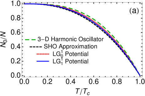
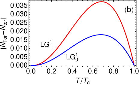
Figure 6: (Color online) (a) Plot of the fraction of particles in the ground state as a function of the scaled temperature. Plotted are the SHO approximation to the LG potentials (black dashed), the LG${}_{1}^{1}$ mode (blue solid), the LG${}_{0}^{1}$ mode (red dot-dashed), and the 3-D isotropic harmonic oscillator (green dotted). (b) The absolute difference in LG${}_{p}^{l}$ fractions and the fraction due to the SHO approximation

where $\beta_{c}=1/k_{B}T_{c}$. Figure 6 (a) shows $N_{0}/N$ as a function of the scaled temperature, $T/T_{c}$ for the LG${}_{0}^{1}$ mode dipole trap (dot-dashed line), the LG${}_{1}^{1}$ mode dipole trap (solid line), the harmonic approximation to a LG${}_{p}^{l}$ mode (dashed line), and the 3-D SHO (dotted line). The trap parameters for the LG${}_{0}^{1}$ mode consist of a laser power of $P_{0}=0.16$ mW and a beam waist of $w=31~{}\mu$m. The trap parameters for the LG${}_{1}^{1}$ mode are $P_{0}=1.3$ mW and a beam waist of $w=58$ mW. Both modes have a laser detuning of $|\Delta|/2\pi=1000$ GHz and have the same trapping frequency, $\omega_{z}=\omega_{r}=2\pi\times 100$ Hz. Note that given the form of the density of states (Equations (16) and (20)), Equation (21) does not depend on the coefficient, $\sigma$, but only on the exponent, $\eta$. Therefore, $N_{0}/N$ is exactly the same for the SHO approximation to either potential.
The 3-D SHO is included in Figure 6 (a) to give a qualitative perspective. The errors associated with making the harmonic approximation of the LG modes are similar to the differences between the multiply connected toroidal geometries and the singly-connected 3-D SHO potential. Figure 6 (b) reports the absolute difference between the two LG modes and their respective harmonic approximations. The harmonic approximation error can reach as high as $3.7\%$ for the LG${}_{0}^{1}$ and $1.8\%$ for the LG${}_{1}^{1}$. Such errors are on the same order as the effects associated with finite system sizes ($N\rightarrow\infty$ approximation) experimentally shown in reference ejm96 . The trap depth is $0.5~{}\mu\textrm{K}$, the beam waist for the LG${}_{0}^{1}$ is $31~{}\mu\textrm{m}$, the beams waist for the LG${}_{1}^{1}$ is $58~{}\mu\textrm{m}$, and the laser detuning is $|\Delta|/2\pi=1000$ GHz. A precise knowledge of the fraction of trapped atoms in the ground state may be necessary for many of the applications of LG laser modes as dipole traps.

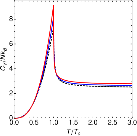
Figure 7: (Color online) Plot of the heat capacity per particle in units of $k_{b}$ for the LG${}_{0}^{1}$ (red), the LG${}_{1}^{1}$ (blue), and the harmonic approximation (black). The heat capacity is a function of the temperature, where $T$ is in units of $T_{c}$. The thermodynamic discontinuity at $T=T_{c}$ indicates a phase transition.

Figure 7 shows the heat capacity for samples trapped in LG${}_{0}^{1}$ (upper curve) and LG${}_{1}^{1}$ (middle curve) with a respective harmonic approximation (lower dashed curve). Like Figure 6, the harmonic approximation can be represented by a single curve because the scaling of the heat capacity and temperature allow for a dependence on a single parameter, $\eta$ in Equation (20). The laser parameters correspond to situations where the confined atoms occupy regions of the trap that deviate from a harmonic description. The disagreement between the LG potentials and the harmonic approximations can be as large as $24\%$ around $T_{c}$.
Toroidal traps are ideal geometries for employment in BEC gyroscope and vortex experiments. Matter-wave interferometers may offer better sensitivity than traditional optical interferometers. Vortices provide a key testing ground for superfluid behavior studies. For these precise applications, BEC characteristics should be well understood. In particular, knowledge of the fraction of trapped atoms in the condensate is important for these applications. In addition, the wave functions of condensates confined in LG traps may need to take into account the full trap geometry.
We calculate the thermal properties of a Bose gas confined by a LG${}_{p}^{l}$ laser dipole trap: the critical transition temperature for a wide range of experimental parameters, the condensate fraction, and the heat capacity. We also compute the thermal properties using a SHO approximation to the potential minimum and compare to the exact results. Depending on the precision required, there exists a regime in which the thermal properties of atoms confined to LG${}_{p}^{l}$ dipole traps contain non-negligible deviations. When the critical temperature is on the order of the trap depth (a depth of $0.1~{}\mu\textrm{K}$), it is predicted to be too high by errors as large as $8\%$. In this regime, the number of atoms in the ground state is underestimated for temperatures below the critical temperature. We also find that the heat capacity contains large deviations around the BEC transition temperature. These corrections are on the order of well known effects (such as finite size corrections).
This work is supported by the Research Corporation, Digital Optics Corporation, and The University of Oklahoma.

References

- (1) F. Dalfovo, S. Giorgini, L. P. Pitaevskii, S. Stringari, Theory of bose-einstein condensation in trapped gases, Rev. Mod. Phys. 71 (3) (1999) 463–512.
- (2) M.-O. Mewes, M. R. Andrews, N. J. van Druten, D. M. Kurn, D. S. Durfee, W. Ketterle, Bose-einstein condensation in a tightly confining dc magnetic trap, Phys. Rev. Lett. 77 (3) (1996) 416–419.
- (3) J. R. Ensher, D. S. Jin, M. R. Matthews, C. E. Wieman, E. A. Cornell, Bose-einstein condensation in a dilute gas: Measurement of energy and ground-state occupation, Phys. Rev. Lett. 77 (25) (1996) 4984–4987.
- (4) F. London, On the bose-einstein condensation, Phys. Rev. 54 (11) (1938) 947–954.
- (5) M. R. Matthews, B. P. Anderson, P. C. Haljan, D. S. Hall, C. E. Wieman, E. A. Cornell, Vortices in a bose-einstein condensate, Phys. Rev. Lett. 83 (13) (1999) 2498–2501.
- (6) K. W. Madison, F. Chevy, W. Wohlleben, J. Dalibard, Vortex formation in a stirred bose-einstein condensate, Phys. Rev. Lett. 84 (5) (2000) 806–809.
- (7) J. R. Abo-Shaeer, C. Raman, J. M. Vogels, W. Ketterle, Observation of vortex lattices in bose-einstein condensates, Science 292 (5516) (2001) 476–479.
- (8) R. Dum, J. I. Cirac, M. Lewenstein, P. Zoller, Creation of dark solitons and vortices in bose-einstein condensates, Phys. Rev. Lett. 80 (14) (1998) 2972–2975.
- (9) P. Capuzzi, D. M. Jezek, Stationary arrays of vortices in bose-einstein condensates confined by a toroidal trap, Journal of Physics B: Atomic, Molecular and Optical Physics 42 (14) (2009) 145301.
- (10) C. Ryu, M. F. Andersen, P. Cladé, V. Natarajan, K. Helmerson, W. D. Phillips, Observation of persistent flow of a bose-einstein condensate in a toroidal trap, Physical Review Letters 99 (26) (2007) 260401.
- (11) B. P. Anderson, K. Dholakia, E. M. Wright, Atomic-phase interference devices based on ring-shaped bose-einstein condensates: Two-ring case, Phys. Rev. A 67 (3) (2003) 033601.
- (12) S. Thanvanthri, K. T. Kapale, J. P. Dowling, Ultra-stable matter-wave gyroscopy with conter-rotating vortex superpositions in bose-einstein condensates, arXiv:0907.1138v1 [quant-ph].
- (13) M. D. Barrett, J. A. Sauer, M. S. Chapman, All-optical formation of an atomic bose-einstein condensate, Phys. Rev. Lett. 87 (1) (2001) 010404.
- (14) R. Onofrio, C. Raman, J. M. Vogels, J. R. Abo-Shaeer, A. P. Chikkatur, W. Ketterle, Observation of superfluid flow in a bose-einstein condensed gas, Phys. Rev. Lett. 85 (11) (2000) 2228–2231.
- (15) A. S. Arnold, E. Riis, Bose-einstein condensates in ’giant’ toroidal magnetic traps, Journal of Modern Optics 49 (2002) 959.
- (16) L. Allen, M. W. Beijersbergen, R. J. C. Spreeuw, J. P. Woerdman, Orbital angular momentum of light and the transformation of laguerre-gaussian laser modes, Phys. Rev. A 45 (11) (1992) 8185–8189.
- (17) K.-P. Marzlin, W. Zhang, E. M. Wright, Vortex coupler for atomic bose-einstein condensates, Phys. Rev. Lett. 79 (24) (1997) 4728–4731.
- (18) R. Kanamoto, E. M. Wright, P. Meystre, Quantum dynamics of raman-coupled bose-einstein condensates using laguerre-gaussian beams, Phys. Rev. A 75 (6) (2007) 063623.
- (19) K. C. Wright, L. S. Leslie, N. P. Bigelow, Optical control of the internal and external angular momentum of a bose-einstein condensate, Phys. Rev. A 77 (4) (2008) 041601.
- (20) L. Salasnich, A. Parola, L. Reatto, Bosons in a toroidal trap: Ground state and vortices, Phys. Rev. A 59 (4) (1999) 2990–2995.
- (21) E. M. Wright, J. Arlt, K. Dholakia, Toroidal optical dipole traps for atomic bose-einstein condensates using laguerre-gaussian beams, Phys. Rev. A 63 (1) (2000) 013608.
-
(22)
T. Tsurumi, M. Wadati, Ground state properties of a toroidally trapped
bose-einstein condensate, Journal of the Physical Society of Japan 70 (6) (2001) 1512–1518. - (23) W. Petrich, M. H. Anderson, J. R. Ensher, E. A. Cornell, Stable, tightly confining magnetic trap for evaporative cooling of neutral atoms, Phys. Rev. Lett. 74 (17) (1995) 3352–3355.
- (24) A. Görlitz, J. M. Vogels, A. E. Leanhardt, C. Raman, T. L. Gustavson, J. R. Abo-Shaeer, A. P. Chikkatur, S. Gupta, S. Inouye, T. Rosenband, W. Ketterle, Realization of bose-einstein condensates in lower dimensions, Phys. Rev. Lett. 87 (13) (2001) 130402.
- (25) V. Bagnato, D. E. Pritchard, D. Kleppner, Bose-einstein condensation in an external potential, Phys. Rev. A 35 (10) (1987) 4354–4358.
- (26) Mathematica Edition: Version 7.0, Wolfram Research, Inc., Champaign, Illinois, 2008.
-
(27)
T. G. Akin, E. R. I. Abraham,
Mathematica
notebook on the bose-einstein condensation transition properties in
laguerre–gaussian dipole traps.
URL http://nhn.nhn.ou.edu/~abe/research/lgbeams/index.html