Resistor network approaches to electrical impedance tomography

Abstract

We review a resistor network approach to the numerical solution of the inverse problem of electrical impedance tomography (EIT). The networks arise in the context of finite volume discretizations of the elliptic equation for the electric potential, on sparse and adaptively refined grids that we call optimal. The name refers to the fact that the grids give spectrally accurate approximations of the Dirichlet to Neumann map, the data in EIT. The fundamental feature of the optimal grids in inversion is that they connect the discrete inverse problem for resistor networks to the continuum EIT problem.

1 Introduction

We consider the inverse problem of electrical impedance tomography (EIT) in two dimensions [11]. It seeks the scalar valued positive and bounded conductivity $\sigma({\bf x})$, the coefficient in the elliptic partial differential equation for the potential $u\in H^{1}(\Omega)$,

$$\nabla\cdot\left[\sigma({\bf x})\nabla u({\bf x})\right]=0,\qquad{\bf x}\in\Omega.$$ (1.1)

The domain $\Omega$ is a bounded and simply connected set in $\mathbb{R}^{2}$ with smooth boundary $\mathcal{B}$. Because all such domains are conformally equivalent by the Riemann mapping theorem, we assume throughout that $\Omega$ is the unit disk,

$$\Omega=\left\{{\bf x}=(r\cos\theta,r\sin\theta),\quad r\in[0,1],~{}~{}\theta\in[0,2\pi)\right\}.$$ (1.2)

The EIT problem is to determine $\sigma({\bf x})$ from measurements of the Dirichlet to Neumann (DtN) map $\Lambda_{\sigma}$ or equivalently, the Neumann to Dirichlet map $\Lambda_{\sigma}^{\dagger}$. We consider the full boundary setup, with access to the entire boundary, and the partial measurement setup, where the measurements are confined to an accessible subset $\mathcal{B}_{A}$ of $\mathcal{B}$, and the remainder $\mathcal{B}_{I}=\mathcal{B}\setminus\mathcal{B}_{A}$ of the boundary is grounded ($u|_{\mathcal{B}_{I}}=0$).

The DtN map $\Lambda_{\sigma}:H^{1/2}(\mathcal{B})\to H^{-1/2}(\mathcal{B})$ takes arbitrary boundary potentials ${u_{{}_{\mathcal{B}}}}$ in the trace space $H^{1/2}(\mathcal{B})$ to normal boundary currents

$$\Lambda_{\sigma}{u_{{}_{\mathcal{B}}}}({\bf x})=\sigma({\bf x}){\bf n}({\bf x})\cdot\nabla u({\bf x}),\qquad{\bf x}\in\mathcal{B},$$ (1.3)

where ${\bf n}({\bf x})$ is the outer normal at ${\bf x}\in\mathcal{B}$ and $u({\bf x})$ solves (1.1) with Dirichlet boundary conditions

$$u({\bf x})={u_{{}_{\mathcal{B}}}}({\bf x}),\quad{\bf x}\in\mathcal{B}.$$ (1.4)

Note that $\Lambda_{\sigma}$ has a null space consisting of constant potentials and thus, it is invertible only on a subset $\mathcal{J}$ of $H^{-1/2}(\mathcal{B})$, defined by

$$\mathcal{J}=\left\{J\in H^{-1/2}(\mathcal{B})~{}~{}\mbox{such that}~{}~{}\int_{\mathcal{B}}J({\bf x})ds({\bf x})=0\right\}.$$ (1.5)

Its generalized inverse is the NtD map $\Lambda_{\sigma}^{\dagger}:\mathcal{J}\to H^{1/2}(\mathcal{B})$, which takes boundary currents ${J}_{{}_{\mathcal{B}}}\in\mathcal{J}$ to boundary potentials

$$\Lambda_{\sigma}^{\dagger}{J}_{{}_{\mathcal{B}}}({\bf x})=u({\bf x}),\qquad{\bf x}\in\mathcal{B}.$$ (1.6)

Here $u$ solves (1.1) with Neumann boundary conditions

$$\sigma({\bf x}){\bf n}({\bf x})\cdot\nabla u({\bf x})={J}_{{}_{\mathcal{B}}}({\bf x}),\qquad{\bf x}\in\mathcal{B},$$ (1.7)

and it is defined up to an additive constant, that can be fixed for example by setting the potential to zero at one boundary point, as if it were connected to the ground.

It is known that $\Lambda_{\sigma}$ determines uniquely $\sigma$ in the full boundary setup [5]. See also the earlier uniqueness results [56, 18] under some smoothness assumptions on $\sigma$. Uniqueness holds for the partial boundary setup as well, at least for $\sigma\in C^{3+\epsilon}(\bar{\Omega})$ and $\epsilon>0$, [39]. The case of real-analytic or piecewise real-analytic $\sigma$ is resolved in [27, 28, 45, 46].

However, the problem is exponentially unstable, as shown in [1, 9, 53]. Given two sufficiently regular conductivities $\sigma_{1}$ and $\sigma_{2}$, the best possible stability estimate is of logarithmic type

$$\|\sigma_{1}-\sigma_{2}\|_{L^{\infty}(\Omega)}\leq c\left|\log\|\Lambda_{\sigma_{1}}-\Lambda_{\sigma_{2}}\|_{H^{1/2}(\mathcal{B}),H^{-1/2}(\mathcal{B})}\right|^{-\alpha},$$ (1.8)

with some positive constants $c$ and $\alpha$. This means that if we have noisy measurements, we cannot expect the conductivity to be close to the true one uniformly in $\Omega$, unless the noise is exponentially small.

In practice the noise plays a role and the inversion can be carried out only by imposing some regularization constraints on $\sigma$. Moreover, we have finitely many measurements of the DtN map and we seek numerical approximations of $\sigma$ with finitely many degrees of freedom (parameters). The stability of these approximations depends on the number of parameters and their distribution in the domain $\Omega$.

It is shown in [2] that if $\sigma$ is piecewise constant, with a bounded number of unknown values, then the stability estimates on $\sigma$ are no longer of the form (1.8), but they become of Lipschitz type. However, it is not really understood how the Lipschitz constant depends on the distribution of the unknowns in $\Omega$. Surely, it must be easier to determine the features of the conductivity near the boundary than deep inside $\Omega$.

Then, the question is how to parametrize the unknown conductivity in numerical inversion so that we can control its stability and we do not need excessive regularization with artificial penalties that introduce artifacts in the results. Adaptive parametrizations for EIT have been considered for example in [43, 50] and [3, 4]. Here we review our inversion approach that is based on resistor networks that arise in finite volume discretizations of (1.1) on sparse and adaptively refined grids which we call optimal. The name refers to the fact that they give spectral accuracy of approximations of $\Lambda_{\sigma}$ on finite volume grids. One of their important features is that they are refined near the boundary, where we make the measurements, and coarse away from it. Thus they capture the expected loss of resolution of the numerical approximations of $\sigma$.

Optimal grids were introduced in [29, 30, 41, 7, 6] for accurate approximations of the DtN map in forward problems. Having such approximations is important for example in domain decomposition approaches to solving second order partial differential equations and systems, because the action of a sub-domain can be replaced by the DtN map on its boundary [61]. In addition, accurate approximations of DtN maps allow truncations of the computational domain for solving hyperbolic problems. The studies in [29, 30, 41, 7, 6] work with spectral decompositions of the DtN map, and show that by just placing grid points optimally in the domain, one can obtain exponential convergence rates of approximations of the DtN map with second order finite difference schemes. That is to say, although the solution of the forward problem is second order accurate inside the computational domain, the DtN map is approximated with spectral accuracy. Problems with piecewise constant and anisotropic coefficients are considered in [31, 8].

The optimal grids are useful in the context of numerical inversion, because they resolve the inconsistency that arises from the exponential ill posedness of the problem and the second order convergence of typical discretization schemes applied to equation (1.1), on ad-hoc grids that are usually uniform. The forward problem for the approximation of the DtN map is the inverse of the EIT problem, so it should converge exponentially. This can be achieved by discretizing on the optimal grids.

In this article we review the use of optimal grids in inversion, as it was developed over the last few years in [12, 14, 13, 37, 15, 16, 52]. We present first, in section 3, the case of layered conductivity $\sigma=\sigma(r)$ and full boundary measurements, where the DtN map has eigenfunctions $e^{ik\theta}$ and eigenvalues denoted by $f(k^{2})$, with integer $k$. Then, the forward problem can be stated as one of rational approximation of $f(\lambda)$, for $\lambda$ in the complex plane, away from the negative real axis. We explain in section 3 how to compute the optimal grid from such rational approximants and also how to use it in inversion. The optimal grid depends on the type of discrete measurements that we make of $\Lambda_{\sigma}$ (i.e., $f(\lambda)$) and so does the accuracy and stability of the resulting approximations of $\sigma$.

The two dimensional problem $\sigma=\sigma(r,\theta)$ is reviewed in sections 4 and 5. The easier case of full access to the boundary, and discrete measurements at $n$ equally distributed points on $\mathcal{B}$ is in section 4. There, the grids are essentially the same as in the layered case and the finite volumes discretization leads to circular networks with topology determined by the grids. We show how to use the discrete inverse problem theory for circular networks developed in [22, 23, 40, 25, 26] for the numerical solution of the EIT problem. Section 5 considers the more difficult, partial boundary measurement setup, where the accessible boundary consists of either one connected subset of $\mathcal{B}$ or two disjoint subsets. There, the optimal grids are truly two dimensional and cannot be computed directly from the layered case.

The theoretical review of our results in [12, 14, 13, 37, 15, 16, 52] is complemented by some numerical results. For brevity, all the results are in the noiseless case. We refer the reader to [17] for an extensive study of noise effects on our inversion approach.

2 Resistor networks as discrete models for EIT

Figure 1: Finite volume discretization on a staggered grid. The primary grid lines are solid and the dual ones are dashed. The primary grid nodes are indicated with $\times$ and the dual nodes with $\circ$. The dual cell $C_{i,j}$, with vertices (dual nodes) $P_{i\pm\frac{1}{2},j\pm\frac{1}{2}}$ surrounds the primary node $P_{i,j}$. A resistor is shown as a rectangle with axis along a primary line, that intersects a dual line at the point indicated with $\Box$.

Resistor networks arise naturally in the context of finite volume discretizations of the elliptic equation (1.1) on staggered grids with interlacing primary and dual lines that may be curvilinear, as explained in section 2.1. Standard finite volume discretizations use arbitrary, usually equidistant tensor product grids. We consider optimal grids that are designed to obtain very accurate approximations of the measurements of the DtN map, the data in the inverse problem. The geometry of these grids depends on the measurement setup. We describe in section 2.2 the type of grids used for the full measurement case, where we have access to the entire boundary $\mathcal{B}$. The grids for the partial boundary measurement setup are discussed later, in section 5.

2.1 Finite volume discretization and resistor networks

See Figure 1 for an illustration of a staggered grid. The potential $u({\bf x})$ in equation (1.1) is discretized at the primary nodes $P_{i,j}$, the intersection of the primary grid lines, and the finite volumes method balances the fluxes across the boundary of the dual cells $C_{ij}$,

$$\int_{C_{i,j}}\nabla\cdot\left[\sigma({\bf x})\nabla u({\bf x})\right]d{\bf x}=\int_{\partial C_{i,j}}\sigma({\bf x}){\bf n}({\bf x})\cdot\nabla u({\bf x})ds({\bf x})=0.$$ (2.1)

A dual cell $C_{i,j}$ contains a primary point $P_{i,j}$, it has vertices (dual nodes) $P_{i\pm\frac{1}{2},j\pm\frac{1}{2}}$, and boundary

$$\partial C_{i,j}=\Sigma_{i,j+\frac{1}{2}}\cup\Sigma_{i+\frac{1}{2},j}\cup\Sigma_{i,j-\frac{1}{2}}\cup\Sigma_{i-\frac{1}{2},j},$$ (2.2)

the union of the dual line segments $\Sigma_{i,j\pm\frac{1}{2}}=(P_{i-\frac{1}{2},j\pm\frac{1}{2}},P_{i+\frac{1}{2},j\pm\frac{1}{2}})$ and $\Sigma_{i\pm\frac{1}{2},j}=(P_{i\pm\frac{1}{2},j-\frac{1}{2}},P_{i\pm\frac{1}{2},j+\frac{1}{2}}).$ Let us denote by $\mathcal{P}=\{P_{i,j}\}$ the set of primary nodes, and define the potential function $U:\mathcal{P}\to\mathbb{R}$ as the finite volume approximation of $u({\bf x})$ at the points in $\mathcal{P}$,

$$U_{i,j}\approx u(P_{i,j}),\qquad P_{i,j}\in\mathcal{P}.$$ (2.3)

The set $\mathcal{P}$ is the union of two disjoint sets $\mathcal{P}_{\mathcal{I}}$ and $\mathcal{P}_{\mathcal{B}}$ of interior and boundary nodes, respectively. Adjacent nodes in $\mathcal{P}$ are connected by edges in the set $\mathcal{E}\subset\mathcal{P}\times\mathcal{P}$. We denote the edges by $E_{i,j\pm\frac{1}{2}}=(P_{i,j},P_{i,j\pm 1})$ and $E_{i\pm\frac{1}{2},j}=(P_{i\pm 1,j},P_{i,j})$.

The finite volume discretization results in a system of linear equations for the potential

$$\gamma_{i+\frac{1}{2},j}(U_{i+1,j}-U_{i,j})+\gamma_{i-\frac{1}{2},j}(U_{i-1,j}-U_{i,j})+\gamma_{i,j+\frac{1}{2}}(U_{i,j+1}-U_{i,j})+\gamma_{i,j-\frac{1}{2}}(U_{i,j-1}-U_{i,j})=0,$$ (2.4)

with terms given by approximations of the fluxes

$$\int_{\Sigma_{i,j\pm\frac{1}{2}}}\sigma({\bf x}){\bf n}({\bf x})\cdot\nabla u({\bf x})ds({\bf x})\approx\gamma_{i,j\pm\frac{1}{2}}(U_{i,j\pm 1}-U_{i,j}),$$

$$\int_{\Sigma_{i\pm\frac{1}{2},j}}\sigma({\bf x}){\bf n}({\bf x})\cdot\nabla u({\bf x})ds({\bf x})\approx\gamma_{i\pm\frac{1}{2},j}(U_{i\pm 1,j}-U_{i,j}).$$ (2.5)

Equations (2.4) are Kirchhoff’s law for the interior nodes in a resistor network $(\Gamma,\gamma)$ with graph $\Gamma=(\mathcal{P},\mathcal{E})$ and conductance function $\gamma:\mathcal{E}\to\mathbb{R}^{+}$, that assigns to an edge like $E_{i\pm\frac{1}{2},j}$ in $\mathcal{E}$ a positive conductance $\gamma_{i\pm\frac{1}{2},j}$. At the boundary nodes we discretize either the Dirichlet conditions (1.4), or the Neumann conditions (1.7), depending on what we wish to approximate, the DtN or the NtD map.

To write the network equations in compact (matrix) form, let us number the primary nodes in some fashion, starting with the interior ones and ending with the boundary ones. Then we can write $\mathcal{P}=\left\{{\bf p}_{q}\right\}$, where ${\bf p}_{q}$ are the numbered nodes. They correspond to points like $P_{i,j}$ in Figure 1. Let also ${{\bf U}_{{}_{\mathcal{I}}}}$ and ${{\bf U}_{{}_{\mathcal{B}}}}$ be the vectors with entries given by the potential at the interior nodes and boundary nodes, respectively. The vector of boundary fluxes is denoted by ${{\bf J}_{{}_{\mathcal{B}}}}$. We assume throughout that there are $n$ boundary nodes, so ${{\bf U}_{{}_{\mathcal{B}}}},{{\bf J}_{{}_{\mathcal{B}}}}\in\mathbb{R}^{n}$. The network equations are

$${\bf K}{\bf U}=\left(\begin{array}[]{c}{\bf 0}\\ {\bf J}_{\mathcal{B}}\end{array}\right),\qquad{\bf U}=\left(\begin{array}[]{c}{\bf U}_{\mathcal{I}}\\ {\bf U}_{\mathcal{B}}\end{array}\right),\qquad{\bf K}=\left(\begin{array}[]{cc}{{\bf K}_{{}_{\mathcal{I}\mathcal{I}}}}&{{\bf K}_{{}_{\mathcal{I}\mathcal{B}}}}\\ {{\bf K}_{{}_{\mathcal{I}\mathcal{B}}}}&{{\bf K}_{{}_{\mathcal{B}\mathcal{B}}}}\end{array}\right),$$ (2.6)

where ${\bf K}=\left(K_{ij}\right)$ is the Kirchhoff matrix with entries

$$K_{i,j}=\left\{\begin{array}[]{cl}-\gamma(E),&\mbox{if}~{}i\neq j\mbox{ and }E=\left({\bf p}_{i},{\bf p}_{j}\right)\in\mathcal{E},\\ 0,&\mbox{if}~{}i\neq j\mbox{ and }\left({\bf p}_{i},{\bf p}_{j}\right)\notin\mathcal{E},\\ \displaystyle\sum_{k:~{}E=\left({\bf p}_{i},{\bf p}_{k}\right)\in\mathcal{E}}\gamma(E),&\mbox{if}~{}i=j.\end{array}\right.$$ (2.7)

In (2.6) we write it in block form, with ${{\bf K}_{{}_{\mathcal{I}\mathcal{I}}}}$ the block with row and column indices restricted to the interior nodes, ${{\bf K}_{{}_{\mathcal{I}\mathcal{B}}}}$ the block with row indices restricted to the interior nodes and column indices restricted to the boundary nodes, and so on. Note that ${\bf K}$ is symmetric, and its rows and columns sum to zero, which is just the condition of conservation of currents.

It is shown in [22] that the potential ${\bf U}$ satisfies a discrete maximum principle. Its minimum and maximum entries are located on the boundary. This implies that the network equations with Dirichlet boundary conditions

$${{\bf K}_{{}_{\mathcal{I}\mathcal{I}}}}{{\bf U}_{{}_{\mathcal{I}}}}=-{{\bf K}_{{}_{\mathcal{I}\mathcal{B}}}}{{\bf U}_{{}_{\mathcal{B}}}}$$ (2.8)

have a unique solution if ${{\bf K}_{{}_{\mathcal{I}\mathcal{B}}}}$ has full rank. That is to say, ${{\bf K}_{{}_{\mathcal{I}\mathcal{I}}}}$ is invertible and we can eliminate ${{\bf U}_{{}_{\mathcal{I}}}}$ from (2.6) to obtain

$${{\bf J}_{{}_{\mathcal{B}}}}=\left({{\bf K}_{{}_{\mathcal{B}\mathcal{B}}}}-{{\bf K}_{{}_{\mathcal{B}\mathcal{I}}}}{\bf K}^{-1}_{{}_{\mathcal{I}\mathcal{I}}}{{\bf K}_{{}_{\mathcal{I}\mathcal{B}}}}\right){{\bf U}_{{}_{\mathcal{B}}}}={\bm{\Lambda}_{\gamma}}{{\bf U}_{{}_{\mathcal{B}}}}.$$ (2.9)

The matrix ${\bm{\Lambda}_{\gamma}}\in\mathbb{R}^{n\times n}$ is the Dirichlet to Neumann map of the network. It takes the boundary potential ${{\bf U}_{{}_{\mathcal{B}}}}$ to the vector ${{\bf J}_{{}_{\mathcal{B}}}}$ of boundary fluxes, and is given by the Schur complement of the block ${{\bf K}_{{}_{\mathcal{B}\mathcal{B}}}}$

$${\bm{\Lambda}_{\gamma}}={{\bf K}_{{}_{\mathcal{B}\mathcal{B}}}}-{{\bf K}_{{}_{\mathcal{B}\mathcal{I}}}}{\bf K}^{-1}_{{}_{\mathcal{I}\mathcal{I}}}{{\bf K}_{{}_{\mathcal{I}\mathcal{B}}}}.$$ (2.10)

The DtN map is symmetric, with nontrivial null space spanned by the vector ${\bf 1}_{\mathcal{B}}\in\mathbb{R}^{n}$ of all ones. The symmetry follows directly from the symmetry of ${\bf K}$. Since the columns of ${\bf K}$ sum to zero, ${\bf K}{\bf 1}={\bf 0}$, where ${\bf 1}$ is the vector of all ones. Then, (2.9) gives ${\bf J}_{\mathcal{B}}={\bf 0}={\bm{\Lambda}_{\gamma}}{\bf 1}_{\mathcal{B}}$, which means that ${\bf 1}_{\mathcal{B}}$ is in the null space of ${\bm{\Lambda}_{\gamma}}$.

The inverse problem for a network $(\Gamma,\gamma)$ is to determine the conductance function $\gamma$ from the DtN map ${\bm{\Lambda}_{\gamma}}$. The graph $\Gamma$ is assumed known, and it plays a key role in the solvability of the inverse problem [22, 23, 40, 25, 26]. More precisely, $\Gamma$ must satisfy a certain criticality condition for the network to be uniquely recoverable from ${\bm{\Lambda}_{\gamma}}$, and its topology should be adapted to the type of measurements that we have. We review these facts in detail in sections 3-5. We also show there how to relate the continuum DtN map $\Lambda_{\sigma}$ to the discrete DtN map ${\bm{\Lambda}_{\gamma}}$. The inversion algorithms in this paper use the solution of the discrete inverse problem for networks to determine approximately the solution $\sigma({\bf x})$ of the continuum EIT problem.

2.2 Tensor product grids for the full boundary measurements setup

& $m_{1/2}=0$ $m_{1/2}=1$

Figure 2: Examples of grids. The primary grid lines are solid and the dual ones are dotted. Both grids have $n=6$ primary boundary points, and index of the layers $\ell=3$. We have the type of grid indexed by $m_{1/2}=0$ on the left and by $m_{1/2}=1$ on the right.

In the full boundary measurement setup, we have access to the entire boundary $\mathcal{B}$, and it is natural to discretize the domain (1.2) with tensor product grids that are uniform in angle, as shown in Figure 2.2. Let

$$\theta_{j}=\frac{2\pi(j-1)}{n},\qquad\widehat{\theta}_{j}=\frac{2\pi\left(j-1/2\right)}{n},\qquad j=1,\ldots,n,$$ (2.11)

be the angular locations of the primary and dual nodes. The radii of the primary and dual layers are denoted by $r_{i}$ and $\widehat{r}_{i}$, and we count them starting from the boundary. We can have two types of grids, so we introduce the parameter $m_{1/2}\in\{0,1\}$ to distinguish between them. We have

$$1=r_{1}=\widehat{r}_{1}>r_{2}>\widehat{r}_{2}>\ldots>r_{\ell}>\widehat{r}_{\ell}>r_{\ell+1}\geq 0$$ (2.12)

when $m_{1/2}=0$, and

$$1=\widehat{r}_{1}=r_{1}>\widehat{r}_{2}>r_{2}>\ldots>r_{\ell}>\widehat{r}_{\ell+1}>r_{\ell+1}\geq 0$$ (2.13)

for $m_{1/2}=1$. In either case there are $\ell+1$ primary layers and $\ell+m_{1/2}$ dual ones, as illustrated in Figure 2.2. We explain in sections 3 and 4 how to place optimally in the interval $[0,1]$ the primary and dual radii, so that the finite volume discretization gives an accurate approximation of the DtN map $\Lambda_{\sigma}$.

The graph of the network is given by the primary grid. We follow [22, 23] and call it a circular network. It has $n$ boundary nodes and $n(2\ell+m_{1/2}-1)$ edges. Each edge is associated with an unknown conductance that is to be determined from the discrete DtN map ${\bm{\Lambda}_{\gamma}}$, defined by measurements of $\Lambda_{\sigma}$, as explained in sections 3 and 4. Since ${\bm{\Lambda}_{\gamma}}$ is symmetric, with columns summing to zero, it contains $n(n-1)/2$ measurements. Thus, we have the same number of unknowns as data points when

$$2\ell+m_{1/2}-1=\frac{n-1}{2},\qquad n=\mbox{odd integer}.$$ (2.14)

This condition turns out to be necessary and sufficient for the DtN map to determine uniquely a circular network, as shown in [26, 23, 13]. We assume henceforth that it holds.

3 Layered media

In this section we assume a layered conductivity function $\sigma(r)$ in $\Omega$, the unit disk, and access to the entire boundary $\mathcal{B}$. Then, the problem is rotation invariant and can be simplified by writing the potential as a Fourier series in the angle $\theta$. We begin in section 3.1 with the spectral decomposition of the continuum and discrete DtN maps and define their eigenvalues, which contain all the information about the layered conductivity. Then, we explain in section 3.2 how to construct finite volume grids that give discrete DtN maps with eigenvalues that are accurate, rational approximations of the eigenvalues of the continuum DtN map. One such approximation brings an interesting connection between a classic Sturm-Liouville inverse spectral problem [34, 19, 38, 54, 55] and an inverse eigenvalue problem for Jacobi matrices [20], as described in sections 3.2.3 and 3.3. This connection allows us to solve the continuum inverse spectral problem with efficient, linear algebra tools. The resulting algorithm is the first example of resistor network inversion on optimal grids proposed and analyzed in [14], and we review its convergence study in section 3.3.

3.1 Spectral decomposition of the continuum and discrete DtN maps

Because equation (1.1) is separable in layered media, we write the potential $u(r,\theta)$ as a Fourier series

$$u(r,\theta)=v_{\mathcal{B}}(0)+\sum_{k\in\mathbb{Z},k\neq 0}v(r,k)e^{ik\theta},$$ (3.1)

with coefficients $v(r,k)$ satisfying the differential equation

$$\frac{r}{\sigma(r)}\frac{d}{dr}\left[r\sigma(r)\frac{dv(r,k)}{dr}\right]-k^{2}v(r,k)=0,\qquad r\in(0,1),$$ (3.2)

and the condition

$$v(0,k)=0.$$ (3.3)

The first term $v_{\mathcal{B}}(0)$ in (3.1) is the average boundary potential

$$v_{\mathcal{B}}(0)=\frac{1}{2\pi}\int_{0}^{2\pi}u(1,\theta)\,d\theta.$$ (3.4)

The boundary conditions at $r=1$ are Dirichlet or Neumann, depending on which map we consider, the DtN or the NtD map.

3.1.1 The DtN map

The DtN map is determined by the potential $v$ satisfying (3.2-3.3), with Dirichlet boundary condition

$$v(1,k)=v_{\mathcal{B}}(k),$$ (3.5)

where $v_{\mathcal{B}}(k)$ are the Fourier coefficients of the boundary potential $u_{\mathcal{B}}(\theta)$. The normal boundary flux has the Fourier series expansion

$$\sigma(1)\frac{\partial u(1,\theta)}{\partial r}=\Lambda_{\sigma}{u_{{}_{\mathcal{B}}}}(\theta)=\sigma(1)\sum_{k\in\mathbb{Z},k\neq 0}\frac{dv(1,k)}{dr}e^{ik\theta},$$ (3.6)

and we assume for simplicity that $\sigma(1)=1$. Then, we deduce formally from (3.6) that $e^{ik\theta}$ are the eigenfunctions of the DtN map $\Lambda_{\sigma}$, with eigenvalues

$$f(k^{2})={\frac{dv(1,k)}{dr}}/{v(1,k)}.$$ (3.7)

Note that $f(0)=0$.

A similar diagonalization applies to the DtN map ${\bm{\Lambda}_{\gamma}}$ of networks arising in the finite volume discretization of (1.1) if the grids are equidistant in angle, as described in section 2.2. Then, the resulting network is layered in the sense that the conductance function is rotation invariant. We can define various quadrature rules in (2.5), with minor changes in the results [15, Section 2.4]. In this section we use the definitions

$$\gamma_{j+\frac{1}{2},q}=\frac{h_{\theta}}{z(r_{j+1})-z(r_{j})}=\frac{h_{\theta}}{\alpha_{j}},\qquad\gamma_{j,q+\frac{1}{2}}=\frac{\widehat{z}(\widehat{r}_{j+1})-\widehat{z}(\widehat{r}_{j})}{h_{\theta}}=\frac{\widehat{\alpha}_{j}}{h_{\theta}},$$ (3.8)

derived in appendix A, where $h_{\theta}=2\pi/n$ and

$$z(r)=\int_{r}^{1}\frac{dt}{t\sigma(t)},\qquad\widehat{z}(r)=\int_{r}^{1}\frac{\sigma(t)}{t}dt.$$ (3.9)

The network equations (2.4) become

$$\frac{1}{\widehat{\alpha}_{j}}\left(\frac{U_{j+1,q}-U_{j,q}}{\alpha_{j}}-\frac{U_{j,q}-U_{j-1,q}}{\alpha_{j-1}}\right)-\frac{2U_{j,q}-U_{j,q+1}-U_{j,q-1}}{h_{\theta}^{2}}=0,$$ (3.10)

and we can write them in block form as

$$\frac{1}{\widehat{\alpha}_{j}}\left(\frac{{\bf U}_{j+1}-{\bf U}_{j}}{\alpha_{j}}-\frac{{\bf U}_{j}-{\bf U}_{j-1}}{\alpha_{j-1}}\right)-\left[-\partial^{2}_{\theta}\right]{\bf U}_{j}={\bf 0},$$ (3.11)

where

$${\bf U}_{j}=\left(U_{j,1},\ldots,U_{j,n}\right)^{T},$$ (3.12)

and $\left[-\partial^{2}_{\theta}\right]$ is the circulant matrix

$$\left[-\partial^{2}_{\theta}\right]=\frac{1}{h^{2}_{\theta}}\left(\begin{array}[]{ccccccc}2&-1&0&\ldots&\ldots&0&-1\\ -1&2&1&0&\ldots&0&0\\ \ddots&\ddots&\ddots&\ddots&\ddots&\ddots&\ddots\\ -1&0&\ldots&\ldots&0&-1&2\end{array}\right),$$ (3.13)

the discretization of the operator $-\partial^{2}_{\theta}$ with periodic boundary conditions. It has the eigenvectors

$$\left[e^{ik\theta}\right]=\left(e^{ik\theta_{1}},\ldots,e^{ik\theta_{n}}\right)^{T},$$ (3.14)

with entries given by the restriction of the continuum eigenfunctions $e^{ik\theta}$ at the primary grid angles. Here $k$ is integer, satisfying $|k|\leq(n-1)/2$, and the eigenvalues are $\omega_{k}^{2}$, where

$$\omega_{k}=|k|\left|\mbox{sinc}\left(\frac{kh_{\theta}}{2}\right)\right|,$$ (3.15)

and $\mbox{sinc}(x)=\sin(x)/x$. Note that $\omega_{k}^{2}\approx k^{2}$ only for $|k|\ll n$.

To determine the spectral decomposition of the discrete DtN map ${\bm{\Lambda}_{\gamma}}$ we proceed as in the continuum and write the potential ${\bf U}_{j}$ as a Fourier sum

$${\bf U}_{j}=v_{\mathcal{B}}(0){\bf 1}_{\mathcal{B}}+\sum_{|k|\leq\frac{n-1}{2},k\neq 0}V_{j}(k)\left[e^{ik\theta}\right],$$ (3.16)

where we recall that ${\bf 1}_{\mathcal{B}}\in\mathbb{R}^{n}$ is a vector of all ones. We obtain the finite difference equation for the coefficients $V_{j}(k)$,

$$\frac{1}{\widehat{\alpha}_{j}}\left(\frac{V_{j+1}(k)-V_{j}(k)}{\alpha_{j}}-\frac{V_{j}(k)-V_{j-1}(k)}{\alpha_{j-1}}\right)-\omega_{k}^{2}V_{j}(k)=0,$$ (3.17)

where $j=2,3,\ldots,\ell$. It is the discretization of (3.2) that takes the form

$$\frac{d}{d\widehat{z}}\left(\frac{dv(z,k)}{dz}\right)-k^{2}v(z,k)=0,$$ (3.18)

in the coordinates (3.9), where we let in an abuse of notation $v(r,k)\leadsto v(z,k)$. The boundary condition at $r=0$ is mapped to

$$\lim_{z\to\infty}v(z,k)=0,$$ (3.19)

and it is implemented in the discretization as $V_{\ell+1}(k)=0.$ At the boundary $r=1$, where $z=0$, we specify $V_{1}(k)$ as some approximation of $v_{\mathcal{B}}(k)$.

The discrete DtN map ${\bm{\Lambda}_{\gamma}}$ is diagonalized in the basis $\{[e^{ik\theta}]\}_{|k|\leq\frac{n-1}{2}}$, and we denote its eigenvalues by $F(\omega^{2}_{k})$. Its definition depends on the type of grid that we use, indexed by $m_{1/2}$, as explained in section 2.2. In the case $m_{1/2}=0$, the first radius next to the boundary is $r_{2}$, and we define the boundary flux at $\widehat{r}_{1}=1$ as $(V_{1}(k)-V_{2}(k))/\alpha_{1}$. When $m_{1/2}=1$, the first radius next to the boundary is $\widehat{r}_{2}$, so to compute the flux at $\widehat{r}_{1}$ we introduce a ghost layer at $r_{0}>1$ and use equation (3.17) for $j=1$ to define the boundary flux as

$$\frac{V_{0}(k)-V_{1}(k)}{\alpha_{o}}=\widehat{\alpha}_{1}\omega_{k}^{2}V_{1}(k)+\frac{V_{1}(k)-V_{2}(k)}{\alpha_{1}}.$$

Therefore, the eigenvalues of the discrete DtN map are

$$F(\omega_{k}^{2})=m_{1/2}\widehat{\alpha}_{1}\omega_{k}^{2}+\frac{V_{1}(k)-V_{2}(k)}{\alpha_{1}V_{1}(k)}.$$ (3.20)

3.1.2 The NtD map

The NtD map $\Lambda_{\sigma}^{\dagger}$ has eigenfunctions $e^{ik\theta}$ for $k\neq 0$ and eigenvalues $f^{\dagger}(k^{2})=1/f(k^{2})$. Equivalently, in terms of the solution $v(z,k)$ of equation (3.18) with boundary conditions (3.19) and

$$-\frac{dv(0,k)}{dz}=\frac{1}{2\pi}\int_{0}^{2\pi}J_{\mathcal{B}}(\theta)e^{-ik\theta}d\theta=\varphi_{{}_{\mathcal{B}}}(k),$$ (3.21)

we have

$$f^{\dagger}(k^{2})=\frac{v(0,k)}{\varphi_{{}_{\mathcal{B}}}(k)}.$$ (3.22)

In the discrete case, let us use the grids with $m_{1/2}=1$. We obtain that the potential $V_{j}(k)$ satisfies (3.17) for $j=1,2,\ldots,\ell$, with boundary conditions

$$-\frac{V_{1}(k)-V_{0}(k)}{\alpha_{0}}=\Phi_{{}_{\mathcal{B}}}(k),\qquad V_{\ell+1}=0.$$ (3.23)

Here $\Phi_{\mathcal{B}}(k)$ is some approximation of $\varphi_{\mathcal{B}}(k)$. The eigenvalues of ${\bm{\Lambda}^{\dagger}_{\gamma}}$ are

$$F^{\dagger}(\omega_{k}^{2})=\frac{V_{1}(k)}{\Phi_{{}_{\mathcal{B}}}(k)}.$$ (3.24)

3.2 Rational approximations, optimal grids and reconstruction mappings

Let us define by analogy to (3.22) and (3.24) the functions

$$f^{\dagger}(\lambda)=\frac{v(0)}{\varphi_{{}_{\mathcal{B}}}},\qquad F^{\dagger}(\lambda)=\frac{V_{1}}{\Phi_{{}_{\mathcal{B}}}},$$ (3.25)

where $v$ solves equation (3.18) with $k^{2}$ replaced by $\lambda$ and $V_{j}$ solves equation (3.17) with $\omega_{k}^{2}$ replaced by $\lambda$. The spectral parameter $\lambda$ may be complex, satisfying $\lambda\in\mathbb{C}\setminus(-\infty,0]$. For simplicity, we suppress in the notation the dependence of $v$ and $V_{j}$ on $\lambda$. We consider in detail the discretizations on grids indexed by $m_{1/2}=1$, but the results can be extended to the other type of grids, indexed by $m_{1/2}=0$.

Lemma 1.

The function $f^{\dagger}(\lambda)$ is of form

$$f^{\dagger}(\lambda)=\int_{-\infty}^{0}\frac{d\mu(t)}{\lambda-t},$$ (3.26)

where $\mu(t)$ is the positive spectral measure on $(-\infty,0]$ of the differential operator $d_{\widehat{z}}d_{z}$, with homogeneous Neumann condition at $z=0$ and limit condition (3.19). The function $F^{\dagger}(\lambda)$ has a similar form

$$F^{\dagger}(\lambda)=\int_{-\infty}^{0}\frac{d\mu^{F}(t)}{\lambda-t},$$ (3.27)

where $\mu^{F}(t)$ is the spectral measure of the difference operator in (3.17) with boundary conditions (3.23).

Proof: The result (3.26) is shown in [44] and it says that $f^{\dagger}(\lambda)$ is essentially a Stieltjes function. To derive the representation (3.27), we write our difference equations in matrix form for ${\bf V}=(V_{1},\ldots,V_{\ell})^{T}$,

$$\left({\bf A}-\lambda{\bf I}\right){\bf V}=-\frac{\Phi_{{}_{\mathcal{B}}}(\lambda)}{\widehat{\alpha}_{1}}{\bf e}_{1}.$$ (3.28)

Here ${\bf I}$ is the $\ell\times\ell$ identity matrix, ${\bf e}_{1}=(1,\ldots,0)^{T}\in\mathbb{R}^{\ell}$ and ${\bf A}$ is the tridiagonal matrix with entries

$$A_{ij}=\left\{\begin{array}[]{lc}-\frac{1}{\widehat{\alpha}_{i}}\left(\frac{1}{\alpha_{i}}+\frac{1}{\alpha_{i-1}}\right)\delta_{i,j}+\frac{1}{\widehat{\alpha}_{i}\alpha_{i-1}}\delta_{i-1,j}+\frac{1}{\widehat{\alpha}_{i}\alpha_{i}}\delta_{i+1,j}{}{}&\mbox{if}~{}1<i\leq\ell,~{}1\leq j\leq\ell,\\ -\frac{1}{\widehat{\alpha}_{1}\alpha_{1}}\delta_{1,j}+\frac{1}{\widehat{\alpha}_{1}\alpha_{1}}\delta_{2,j}&\mbox{if}~{}i=1,~{}1\leq j\leq\ell.\end{array}\right.$$ (3.29)

The Kronecker delta symbol $\delta_{i,j}$ is one when $i=j$ and zero otherwise. Note that ${\bf A}$ is a Jacobi matrix when it is defined on the vector space $\mathbb{R}^{\ell}$ with weighted inner product

$$\left<{\bf a},{\bf b}\right>=\sum_{j=1}^{\ell}\widehat{\alpha}_{j}a_{j}b_{j},\qquad{\bf a}=(a_{1},\ldots,a_{\ell})^{T},~{}~{}{\bf b}=(b_{1},\ldots,b_{\ell})^{T}.$$ (3.30)

That is to say,

$$\widetilde{\bf A}=\mbox{diag}\left(\widehat{\alpha}_{1}^{1/2},\ldots,\widehat{\alpha}_{\ell}^{1/2}\right){\bf A}\,\mbox{diag}\left(\widehat{\alpha}_{1}^{-1/2},\ldots,\widehat{\alpha}_{\ell}^{-1/2}\right)$$ (3.31)

is a symmetric, tridiagonal matrix, with negative entries on its diagonal and positive entries on its upper/lower diagonal. It follows from [20] that ${\bf A}$ has simple, negative eigenvalues $-\delta^{2}_{j}$ and eigenvectors ${\bf Y}_{j}=\left(Y_{1,j},\ldots,Y_{\ell,j}\right)^{T}$ that are orthogonal with respect to the inner product (3.30). We order the eigenvalues as

$$\delta_{1}<\delta_{2}<\ldots<\delta_{\ell},$$ (3.32)

and normalize the eigenvectors

$$\|{\bf Y}_{j}\|^{2}=\left<{\bf Y}_{j},{\bf Y}_{j}\right>=\sum_{p=1}^{\ell}\widehat{\alpha}_{p}^{2}Y_{p,j}^{2}=1.$$ (3.33)

Then, we obtain from (3.25) and (3.28), after expanding ${\bf V}$ in the basis of the eigenvectors, that

$$F^{\dagger}(\lambda)=\sum_{j=1}^{\ell}\frac{Y_{1,j}^{2}}{\lambda+\delta_{j}^{2}}.$$ (3.34)

This is precisely (3.27), for the discrete spectral measure

$$\mu^{F}(t)=-\sum_{j=1}^{\ell}\xi_{j}H\left(-t-\delta_{j}^{2}\right),\qquad\xi_{j}=Y_{1,j}^{2},$$ (3.35)

where $H$ is the Heaviside step function. $\Box$.

Note that any function of the form (3.34) defines the eigenvalues $F^{\dagger}(\omega_{k}^{2})$ of the NtD map ${\bm{\Lambda}^{\dagger}_{\gamma}}$ of a finite volumes scheme with $\ell+1$ primary radii and uniform discretization in angle. This follows from the decomposition in section 3.1 and the results in [44]. Note also that there is an explicit, continued fraction representation of $F^{\dagger}(\lambda)$, in terms of the network conductances, i.e., the parameters $\alpha_{j}$ and $\widehat{\alpha}_{j}$,

$$F^{\dagger}(\lambda)=\cfrac{1}{\widehat{\alpha}_{1}\lambda+\cfrac{1}{\alpha_{1}+\dots\cfrac{1}{\widehat{\alpha}_{\ell}\lambda+\cfrac{1}{\alpha_{\ell}}}}}.$$ (3.36)

This representation is known in the theory of rational function approximations [59, 44] and its derivation is given in appendix B.

Since both $f^{\dagger}(\lambda)$ and $F^{\dagger}(\lambda)$ are Stieltjes functions, we can design finite volume schemes (i.e., layered networks) with accurate, rational approximations $F^{\dagger}(\lambda)$ of $f^{\dagger}(\lambda)$. There are various approximants $F^{\dagger}(\lambda)$, with different rates of convergence to $f^{\dagger}(\lambda)$, as $\ell\to\infty$. We discuss two choices below, in sections 3.2.2 and 3.2.3, but refer the reader to [30, 29, 32] for details on various Padé approximants and the resulting discretization schemes. No matter which approximant we choose, we can compute the network conductances, i.e., the parameters $\alpha_{j}$ and $\widehat{\alpha}_{j}$ for $j=1,\ldots,\ell$, from $2\ell$ measurements of $f^{\dagger}(\lambda)$. The type of measurements dictates the type of approximant, and only some of them are directly accessible in the EIT problem. For example, the spectral measure $\mu(\lambda)$ cannot be determined in a stable manner in EIT. However, we can measure the eigenvalues $f^{\dagger}(k^{2})$ for integer $k$, and thus we can design a rational, multi-point Padé approximant.

Remark 1.

We describe in detail in appendix D how to determine the parameters $\{\alpha_{j},\widehat{\alpha}_{j}\}_{j=1,\ldots,\ell}$ from $2\ell$ point measurements of $f^{\dagger}(\lambda)$, such as $f^{\dagger}(k^{2})$, for $k=1,\ldots,\frac{n-1}{2}=2\ell$. The are two steps. The first is to write $F^{\dagger}(\lambda)$ as the ratio of two polynomials of $\lambda$, and determine the $2\ell$ coefficients of these polynomials from the measurements $F^{\dagger}(\omega_{k}^{2})$ of $f^{\dagger}(k^{2})$, for $1\leq k\leq\frac{n-1}{2}$. See section 3.2.2 for examples of such measurements. The exponential instability of EIT comes into play in this step, because it involves the inversion of a Vandermonde matrix. It is known [33] that such matrices have condition numbers that grow exponentially with the dimension $\ell$. The second step is to determine the parameters $\{\alpha_{j},\widehat{\alpha}_{j}\}_{j=1,\ldots,\ell}$ from the coefficients of the polynomials. This can be done in a stable manner with the Euclidean division algorithm [47].

The approximation problem can also be formulated in terms of the DtN map, with $F(\lambda)=1/F^{\dagger}(\lambda)$. Moreover, the representation (3.36) generalizes to both types of grids, by replacing $\widehat{\alpha}_{1}\lambda$ with $\widehat{\alpha}_{1}m_{1/2}\lambda$. Recall equation (3.20) and note the parameter $\widehat{\alpha}_{1}$ does not play any role when $m_{1/2}=0$.

3.2.1 Optimal grids and reconstruction mappings

Once we have determined the network conductances, that is the coefficients

$$\alpha_{j}=\int_{r_{j+1}}^{r_{j}}\frac{dr}{r\sigma(r)},\qquad\widehat{\alpha}_{j}=\int_{\widehat{r}_{j+1}}^{\widehat{r}_{j}}\frac{\sigma(r)}{r}dr,\qquad j=1,\ldots,\ell,$$ (3.37)

we could determine the optimal placement of the radii $r_{j}$ and $\widehat{r}_{j}$, if we knew the conductivity $\sigma(r)$. But $\sigma(r)$ is the unknown in the inverse problem. The key idea behind the resistor network approach to inversion is that the grid depends only weakly on $\sigma$, and we can compute it approximately for the reference conductivity $\sigma^{(o)}\equiv 1$.

Let us denote by $f^{\dagger(o)}(\lambda)$ the analog of (3.25) for conductivity $\sigma^{(o)}$, and let $F^{\dagger(o)}(\lambda)$ be its rational approximant defined by (3.36), with coefficients $\alpha^{(o)}_{j}$ and $\widehat{\alpha}^{(o)}_{j}$ given by

$$\alpha^{(o)}_{j}=\int_{r^{(o)}_{j+1}}^{r^{(o)}_{j}}\frac{dr}{r}=\log\frac{r^{(o)}_{j}}{r^{(o)}_{j+1}},\qquad\widehat{\alpha}^{(o)}_{j}=\int_{\widehat{r}_{j+1}}^{\widehat{r}_{j}}\frac{dr}{r}=\log\frac{\widehat{r}^{(o)}_{j}}{\widehat{r}^{(o)}_{j+1}},\qquad j=1,\ldots,\ell.$$ (3.38)

Since $r^{(o)}_{1}=\widehat{r}^{(o)}_{1}=1$, we obtain

$$r^{(o)}_{j+1}=\exp\left(-\sum_{q=1}^{j}\alpha^{(o)}_{q}\right),\qquad\widehat{r}^{(o)}_{j+1}=\exp\left(-\sum_{q=1}^{j}\widehat{\alpha}^{(o)}_{q}\right),\qquad j=1,\ldots,\ell.$$ (3.39)

We call the radii (3.39) optimal. The name refers to the fact that finite volume discretizations on grids with such radii give an NtD map that matches the measurements of the continuum map $\Lambda_{\sigma^{(o)}}^{\dagger}$ for the reference conductivity $\sigma^{(o)}$.

Remark 2.

It is essential that the parameters $\{\alpha_{j},\widehat{\alpha}_{j}\}$ and $\{\alpha^{(o)}_{j},\widehat{\alpha}^{(o)}_{j}\}$ are computed from the same type of measurements. For example, if we measure $f^{\dagger}(k^{2})$, we compute $\{\alpha_{j},\widehat{\alpha}_{j}\}$ so that

$$F^{\dagger}(\omega_{k}^{2})=f^{\dagger}(k^{2}),$$

and $\{\alpha^{(o)}_{j},\widehat{\alpha}^{(o)}_{j}\}$ so that

$$F^{\dagger(o)}(\omega_{k}^{2})=f^{\dagger(o)}(k^{2}),$$

where $k=1,\ldots,(n-1)/2$. This is because the distribution of the radii (3.39) in the interval $[0,1]$ depends on what measurements we make, as illustrated with examples in sections 3.2.2 and 3.2.3.

Now let us denote by $\mathcal{D}_{n}$ the set in $\mathbb{R}^{\frac{n-1}{2}}$ of measurements of $f^{\dagger}(\lambda)$, and introduce the reconstruction mapping $\mathcal{Q}_{n}$ defined on $\mathcal{D}_{n}$, with values in $\mathbb{R}_{+}^{\frac{n-1}{2}}$. It takes the measurements of $f^{\dagger}(\lambda)$ and returns the $(n-1)/2$ positive numbers

$$\sigma_{j+1-m_{1/2}} = \frac{\widehat{\alpha}_{j}}{\widehat{\alpha}^{(o)}_{j}},\quad j=2-m_{1/2},\ldots\ell,$$

$$\widehat{\sigma}_{j+m_{1/2}} = \frac{\alpha^{(o)}_{j}}{\alpha_{j}},\quad j=1,2,\ldots,\ell.,$$ (3.40)

where we recall the relation (2.14) between $\ell$ and $n$. We call $\mathcal{Q}_{n}$ a reconstruction mapping because if we take $\sigma_{j}$ and $\widehat{\sigma}_{j}$ as point values of a conductivity at nodes $r^{(o)}_{j}$ and $\widehat{r}^{(o)}_{j}$, and interpolate them on the optimal grid, we expect to get a conductivity that is close to the interpolation of the true $\sigma(r)$. This is assuming that the grid does not depend strongly on $\sigma(r)$. The proof that the resulting sequence of conductivity functions indexed by $\ell$ converges to the true $\sigma(r)$ as $\ell\to\infty$ is carried out in [14], given the spectral measure of $f^{\dagger}(\lambda)$. We review it in section 3.3, and discuss the measurements in section 3.2.3. The convergence proof for other measurements remains an open question, but the numerical results indicate that the result should hold. Moreover, the ideas extend to the two dimensional case, as explained in detail in sections 4 and 5.

3.2.2 Examples of rational interpolation grids

Let us begin with an example that arises in the discretization of the problem with lumped current measurements

$$J_{q}=\frac{1}{h_{\theta}}\int_{\widehat{\theta}_{q}}^{\widehat{\theta}_{q+1}}\Lambda_{\sigma}u_{\mathcal{B}}(\theta)d\theta,$$

for $h_{\theta}=\frac{2\pi}{n}$, and vector ${\bf U}_{\mathcal{B}}=\left(u_{\mathcal{B}}(\theta_{1}),\ldots,u_{\mathcal{B}}(\theta_{n})\right)^{T}$ of boundary potentials. If we take harmonic boundary excitations $u_{\mathcal{B}}(\theta)=e^{ik\theta}$, the eigenfunction of $\Lambda_{\sigma}$ for eigenvalue $f(k^{2})$, we obtain

$$J_{q}=\frac{1}{h_{\theta}}\int_{\widehat{\theta}_{q}}^{\widehat{\theta}_{q+1}}\Lambda_{\sigma}e^{ik\theta}d\theta=f(k^{2})\left|\mbox{sinc}\left(\frac{kh_{\theta}}{2}\right)\right|e^{ik\theta_{q}}=\frac{f(k^{2})}{|k|}\omega_{k}e^{ik\theta_{q}},\qquad q=1,\ldots,n.$$ (3.41)

These measurements, for all integers $k$ satisfying $|k|\leq\frac{n-1}{2}$, define a discrete DtN map ${\bf M}_{n}(\Lambda_{\sigma})$. It is a symmetric matrix with eigenvectors $[e^{ik\theta}]=\left(e^{ik\theta_{1}},\ldots,e^{ik\theta_{n}}\right)^{T}$, and eigenvalues $\frac{f(k^{2})}{|k|}\omega_{k}$.

The approximation problem is to find the finite volume discretization with DtN map ${\bm{\Lambda}_{\gamma}}={\bf M}_{n}(\Lambda_{\sigma})$. Since both ${\bm{\Lambda}_{\gamma}}$ and ${\bf M}_{n}$ have the same eigenvectors, this is equivalent to the rational approximation problem of finding the network conductances (3.8) (i.e., $\alpha_{j}$ and $\widehat{\alpha}_{j}$), so that

$$F(\omega_{k}^{2})=\frac{f(k^{2})}{|k|}\omega_{k},\qquad k=1,\ldots,\frac{n-1}{2}.$$ (3.42)

The eigenvalues depend only on $|k|$, and the case $k=0$ gives no information, because it corresponds to constant boundary potentials that lie in the null space of the DtN map. This is why we take in (3.42) only the positive values of $k$, and obtain the same number $(n-1)/2$ of measurements as unknowns: $\{\alpha_{j}\}_{j=1,\ldots,\ell}$ and $\{\widehat{\alpha}_{j}\}_{j=2-m_{1/2},\ldots,\ell}$.

When we compute the optimal grid, we take the reference $\sigma^{(o)}\equiv 1$, in which case $f^{(o)}(k^{2})=|k|$. Thus, the optimal grid computation reduces to that of rational interpolation of $f(\lambda)$,

$$F^{(o)}(\omega_{k}^{2})=\omega_{k}=f^{(o)}(\omega_{k}^{2}),\qquad k=1,\ldots,\frac{n-1}{2}.$$ (3.43)

This is solved explicitly in [10]. For example, when $m_{1/2}=1$, the coefficients $\alpha^{(o)}_{j}$ and $\widehat{\alpha}^{(o)}_{j}$ are given by

$$\alpha^{(o)}_{j} = h_{\theta}\cot\left[\frac{h_{\theta}}{2}(2\ell-2j+1)\right],\qquad\widehat{\alpha}^{(o)}_{j}=h_{\theta}\cot\left[\frac{h_{\theta}}{2}(2\ell-2j+2)\right],\qquad j=1,2\ldots,\ell,$$ (3.44)

and the radii follow from (3.39). They satisfy the interlacing relations

$$1=\widehat{r}^{(o)}_{1}=r^{(o)}_{1}>\widehat{r}^{(o)}_{2}>r^{(o)}_{2}>\ldots>\widehat{r}^{(o)}_{\ell+1}>r^{(o)}_{\ell+1}\geq 0,$$ (3.45)

as can be shown easily using the monotonicity of the cotangent and exponential functions. We show an illustration of the resulting grids in red, in Figure 3. Note the refinement toward the boundary $r=1$ and the coarsening toward the center $r=0$ of the disk. Note also that the dual points shown with $\circ$ are almost half way between the primary points shown with $\times$. The last primary radii $r^{(o)}_{\ell+1}$ are small, but the points do not reach the center of the domain at $r=0$.

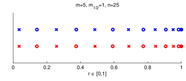
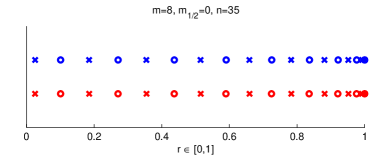
Figure 3: Examples of optimal grids with $n$ equidistant boundary points and primary and dual radii shown with $\times$ and $\circ$. On the left we have $n=25$ and a grid indexed by $m_{1/2}=1$, with $\ell=m+1=6$. On the right we have $n=35$ and a grid indexed by $m_{1/2}=0$, with $\ell=m+1=8.$ The grid shown in red is computed with formulas (3.44). The grid shown in blue is obtained from the rational approximation (3.50).

In sections 4 and 5 we work with slightly different measurements of the DtN map ${\bm{\Lambda}_{\gamma}}={\bf M}_{n}(\Lambda_{\sigma})$, with entries defined by

$$\left({\bm{\Lambda}_{\gamma}}\right)_{p,q}=\int_{0}^{2\pi}\chi_{p}(\theta)\Lambda_{\sigma}\chi_{q}(\theta)d\theta,\qquad p\neq q,\qquad\left({\bm{\Lambda}_{\gamma}}\right)_{p,p}=-\sum_{q\neq p}\left({\bm{\Lambda}_{\gamma}}\right)_{p,q},$$ (3.46)

using the non-negative measurement (electrode) functions $\chi_{q}(\theta)$ that are compactly supported in $(\widehat{\theta}_{q},\widehat{\theta}_{q+1})$, and are normalized by

$$\int_{0}^{2\pi}\chi_{q}(\theta)d\theta=1.$$

For example, we can take

$$\chi_{q}(\theta)=\left\{\begin{array}[]{ll}\frac{1}{h_{\theta}},&\mbox{if}~{}~{}\widehat{\theta}_{q}<\theta<\widehat{\theta}_{q+1},\\ 0,&\mbox{otherwise}.\end{array}\right.,$$

and obtain after a calculation given in appendix C that the entries of ${\bm{\Lambda}_{\gamma}}$ are given by

$$\left({\bm{\Lambda}_{\gamma}}\right)_{p,q}=\frac{1}{2\pi}\sum_{k\in\mathbb{Z}}e^{ik(\theta_{p}-\theta_{q})}f(k^{2})\left[\mbox{sinc}\left(\frac{kh_{\theta}}{2}\right)\right]^{2},\qquad p,q,=1,\ldots,n.$$ (3.47)

We also show in appendix C that

$${\bm{\Lambda}_{\gamma}}\left[e^{ik\theta}\right]=\frac{1}{h_{\theta}}\widetilde{F}(\omega_{k}^{2})\left[e^{ik\theta}\right],\qquad|k|\leq\frac{n-1}{2},$$ (3.48)

with eigenvectors $\left[e^{ik\theta}\right]$ defined in (3.14) and scaled eigenvalues

$$\widetilde{F}(\omega_{k}^{2})=f(k^{2})\left[\mbox{sinc}\left(\frac{kh_{\theta}}{2}\right)\right]^{2}=F(\omega_{k}^{2})\left|\mbox{sinc}\left(\frac{kh_{\theta}}{2}\right)\right|.$$ (3.49)

Here we recalled (3.42) and (3.15).

There is no explicit formula for the optimal grid satisfying

$$\widetilde{F}^{(o)}(\omega_{k}^{2})=F^{(o)}(\omega_{k}^{2})\left|\mbox{sinc}\left(\frac{kh_{\theta}}{2}\right)\right|=\omega_{k}\left|\mbox{sinc}\left(\frac{kh_{\theta}}{2}\right)\right|,$$ (3.50)

but we can compute it as explained in Remark 1 and appendix D. We show in Figure 3 two examples of the grids, and note that they are very close to those obtained from the rational interpolation (3.43). This is not surprising because the sinc factor in (3.50) is not significantly different from $1$ over the range $|k|\leq\frac{n-1}{2}$,

$$\frac{2}{\pi}<\frac{\sin\left[\frac{\pi}{2}\left(1-\frac{1}{n}\right)\right]}{\frac{\pi}{2}\left(1-\frac{1}{n}\right)}\leq\left|\mbox{sinc}\left(\frac{kh_{\theta}}{2}\right)\right|\leq 1.$$

Thus, many eigenvalues $\widetilde{F}^{(o)}(\omega_{k}^{2})$ are approximately equal to $\omega_{k}$, and this is why the grids are similar.

3.2.3 Truncated measure and optimal grids

Another example of rational approximation arises in a modified problem, where the positive spectral measure $\mu$ in Lemma 1 is discrete

$$\mu(t)=-\sum_{j=1}^{\infty}\xi_{j}H\left(-t-\delta_{j}^{2}\right).$$ (3.51)

This does not hold for equation (3.2) or equivalently (3.18), where the origin of the disc $r=0$ is mapped to $\infty$ in the logarithmic coordinates $z(r)$, and the measure $\mu(t)$ is continuous. To obtain a measure like (3.51), we change the problem here and in the next section to

$$\frac{r}{\sigma(r)}\frac{d}{dr}\left[r\sigma(r)\frac{dv(r)}{dr}\right]-\lambda v(r)=0,\qquad r\in(\epsilon,1),$$ (3.52)

with $\epsilon\in(0,1)$ and boundary conditions

$$\frac{\partial v(o)}{\partial r}=\varphi_{\mathcal{B}},\qquad v(\epsilon)=0.$$ (3.53)

The Dirichlet boundary condition at $r=\epsilon$ may be realized if we have a perfectly conducting medium in the disk concentric with $\Omega$ and of radius $\epsilon$. Otherwise, $v(\epsilon)=0$ gives an approximation of our problem, for small but finite $\epsilon$.

Coordinate change and scaling

It is convenient here and in the next section to introduce the scaled logarithmic coordinate

$$\zeta(r)=\frac{z^{(o)}(r)}{Z}=\frac{1}{Z}\int_{r}^{1}\frac{dt}{t},\qquad Z=-\log(\epsilon)=z^{(o)}(\epsilon),$$ (3.54)

and write (3.9) in the scaled form

$$\frac{z(r)}{Z}=\int_{0}^{\zeta}\frac{dt}{\sigma(r(t))}=z^{\prime}(\zeta),\qquad\frac{\widehat{z}(r)}{Z}=\int_{0}^{\zeta}\sigma(r(t))dt=\widehat{z}{\,{}^{\prime}}(\zeta).$$ (3.55)

The conductivity function in the transformed coordinates is

$$\sigma^{\prime}(\zeta)=\sigma(r(\zeta)),\qquad r(\zeta)=e^{-Z\zeta},$$ (3.56)

and the potential

$$v^{\prime}(z^{\prime})=\frac{v(r(z^{\prime}))}{\varphi_{\mathcal{B}}}$$ (3.57)

satisfies the scaled equations

$$\frac{d}{d\widehat{z}^{\,{}^{\prime}}}\left(\frac{dv^{\prime}}{dz^{\prime}}\right)-\lambda^{\prime}v^{\prime} = 0,\quad z^{\prime}\in(0,L^{\prime}),$$

$$\frac{dv(0)}{dz^{\prime}} = -1,\qquad v(L^{\prime})=0,$$ (3.58)

where we let $\lambda^{\prime}=\lambda/Z^{2}$ and

$$L^{\prime}=z^{\prime}(1)=\int_{0}^{1}\frac{dt}{\sigma^{\prime}(t)}.$$ (3.59)

Remark 3.

We assume in the remainder of this section and in section 3.3 that we work with the scaled equations (3.58) and drop the primes for simplicity of notation.

The inverse spectral problem

The differential operator $\frac{d}{d\widehat{z}}\frac{d}{dz}$ acting on the vector space of functions with homogeneous Neumann conditions at $z=0$ and Dirichlet conditions at $z=L$ is symmetric with respect to the weighted inner product

$$\left(a,b\right)=\int_{0}^{\widehat{L}}a(z)b(z)d\widehat{z}=\int_{0}^{1}a(z(\zeta))b(z(\zeta))\sigma(\zeta)d\zeta,\qquad\widehat{L}=\widehat{z}(1).$$ (3.60)

It has negative eigenvalues $\{-\delta_{j}^{2}\}_{j=1,2,\ldots}$, the points of increase of the measure (3.51), and eigenfunctions $y_{j}(z)$. They are orthogonal with respect to the inner product (3.60), and we normalize them by

$$\|y_{j}\|^{2}=\left(y_{j},y_{j}\right)=\int_{0}^{\widehat{L}}y_{j}^{2}(z)d\widehat{z}=1.$$ (3.61)

The weights $\xi_{j}$ in (3.51) are defined by

$$\xi_{j}=y_{j}^{2}(0).$$ (3.62)

For the discrete problem we assume in the remainder of the section that $m_{1/2}=1$, and work with the NtD map, that is with $F^{\dagger}(\lambda)$ represented in Lemma 1 in terms of the discrete measure $\mu^{F}(t)$. Comparing (3.51) and (3.35), we note that we ask that $\mu^{F}(t)$ be the truncated version of $\mu(t)$, given the first $\ell$ weights $\xi_{j}$ and eigenvalues $-\delta_{j}^{2}$, for $j=1,\ldots,\ell$. We arrived at the classic inverse spectral problem [34, 19, 38, 54, 55], that seeks an approximation of the conductivity $\sigma$ from the truncated measure. We can solve it using the theory of resistor networks, via an inverse eigenvalue problem [20] for the Jacobi like matrix ${\bf A}$ defined in (3.29). The key ingredient in the connection between the continuous and discrete eigenvalue problems is the optimal grid, as was first noted in [12] and proved in [14]. We review this result in section 3.3.

The truncated measure optimal grid

The optimal grid is obtained by solving the discrete inverse problem with spectral data for the reference conductivity $\sigma^{(o)}(\zeta)$,

$$\mathcal{D}^{(o)}_{n}=\left\{\xi^{(o)}_{j}=2,\delta^{(o)}_{j}=\pi\left(j-\frac{1}{2}\right),\quad j=1,\ldots,\ell\right\}.$$ (3.63)

The parameters $\{\alpha^{(o)}_{j},\widehat{\alpha}^{(o)}_{j}\}_{j=1,\ldots,\ell}$ can be determined from $\mathcal{D}^{(o)}_{n}$ with the Lanczos algorithm [65, 20] reviewed briefly in appendix E. The grid points are given by

$$\zeta^{(o)}_{j+1}=\alpha^{(o)}_{j}+\zeta^{(o)}_{j}=\sum_{q=1}^{j}\alpha^{(o)}_{q},\qquad\widehat{\zeta}^{(o)}_{j+1}=\widehat{\alpha}^{(o)}_{j}+\widehat{\zeta}^{(o)}_{j}=\sum_{q=1}^{j}\widehat{\alpha}^{(o)}_{q},\qquad j=1,\ldots,\ell,$$ (3.64)

where $\zeta^{(o)}_{1}=\widehat{\zeta}^{(o)}_{1}=0$. This is in the logarithmic coordinates that are related to the optimal radii as in (3.56). The grid is calculated explicitly in [14, Appendix A]. We summarize its properties in the next lemma, for large $\ell$.

Lemma 2.

The steps $\{\alpha^{(o)}_{j},\widehat{\alpha}^{(o)}_{j}\}_{j=1,\ldots,\ell}$ of the truncated measure optimal grid satisfy the monotone relation

$$\widehat{\alpha}^{(o)}_{1}<\alpha^{(o)}_{1}<\widehat{\alpha}^{(o)}_{2}<\alpha^{(o)}_{2}<\ldots<\widehat{\alpha}^{(o)}_{k}<\alpha^{(o)}_{k}.$$ (3.65)

Moreover, for large $\ell$, the primary grid steps are

$$\alpha^{(o)}_{j}=\left\{\begin{array}[]{ll}\frac{2+O\left[(\ell-j)^{-1}+j^{-2}\right]}{\pi\sqrt{\ell^{2}-j^{2}}},&\mbox{if}~{}1\leq j\leq\ell-1,\vspace{0.05in}\\ \frac{\sqrt{2}+O(\ell^{-1})}{\sqrt{\pi\ell}},&\mbox{if}~{}j=\ell,\end{array}\right.$$ (3.66)

and the dual grid steps are

$$\widehat{\alpha}^{(o)}_{j}=\frac{2+O\left[(\ell+1-j)^{-1}+j^{-2}\right]}{\pi\sqrt{\ell^{2}-(j-1/2)^{2}}},\quad 1\leq j\leq\ell.$$ (3.67)

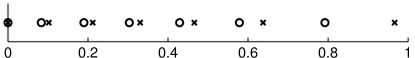
Figure 4: Example of truncated measure optimal grid with $\ell=6$. This is in the logarithmic scaled coordinates $\zeta\in[0,1]$. The primary points are denoted with $\times$ and the dual ones with $\circ$.

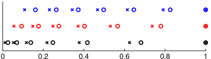
Figure 5: The radial grid obtained with the coordinate change $r=e^{-Z\zeta}$. The scale $Z=-\log\epsilon$ affects the distribution of the radii. The choice $\epsilon=0.1$ is in blue, $\epsilon=0.05$ is in red and $\epsilon=0.01$ is in black. The primary radii are indicated with $\times$ and the dual ones with $\circ$.

We show in Figure 4 an example for the case $\ell=6$. To compare it with the grid in Figure 3, we plot in Figure 5 the radii given by the coordinate transformation (3.56), for three different parameters $\epsilon$. Note that the primary and dual points are interlaced, but the dual points are not half way between the primary points, as was the case in Figure 3. Moreover, the grid is not refined near the boundary at $r=1$. In fact, there is accumulation of the grid points near the center of the disk, where we truncate the domain. The smaller the truncation radius $\epsilon$, the larger the scale $Z=-\log\epsilon$, and the more accumulation near the center.

Intuitively, we can say that the grids in Figure 3 are much superior to the ones computed from the truncated measure, for both the forward and inverse EIT problem. Indeed, for the forward problem, the rate of convergence of $F^{\dagger}(\lambda)$ to $f^{\dagger}(\lambda)$ on the truncated measure grids is algebraic [14]

$$\left|f^{\dagger}(\lambda)-F^{\dagger}(\lambda)\right|=\left|\sum_{j=\ell+1}^{\infty}\frac{\xi_{j}}{\lambda+\delta_{j}^{2}}\right|=O\left(\sum_{j=\ell+1}^{\infty}\frac{1}{j^{2}}\right)=O\left(\frac{1}{\ell}\right).$$

The rational interpolation grids described in section 3.2.2 give exponential convergence of $F^{\dagger}(\lambda)$ to $f^{\dagger}(\lambda)$ [51]. For the inverse problem, we expect that the resolution of reconstructions of $\sigma$ decreases rapidly away from the boundary where we make the measurements, so it makes sense to invert on grids like those in Figure 3, that are refined near $r=1$.

The examples in Figures 3 and 5 show the strong dependence of the grids on the measurement setup. Although the grids in Figure 5 are not good for the EIT problem, they are optimal for the inverse spectral problem. The optimality is in the sense that the grids give an exact match of the spectral measurements (3.63) of the NtD map for conductivity $\sigma^{(o)}$. Furthermore, they give a very good match of the spectral measurements (3.68) for the unknown $\sigma$, and the reconstructed conductivity on them converges to the true $\sigma$, as we show next.

3.3 Continuum limit of the discrete inverse spectral problem on optimal grids

Let $\mathcal{Q}_{n}:\mathcal{D}_{n}\to\mathbb{R}_{+}^{2\ell}$ be the reconstruction mapping that takes the data

$$\mathcal{D}_{n}=\left\{\xi_{j},\delta_{j},\quad j=1,\ldots,\ell\right\}$$ (3.68)

to the $2\ell=\frac{n-1}{2}$ positive values $\{\sigma_{j},\widehat{\sigma}_{j}\}_{j=1,\ldots,\ell}$ given by

$$\sigma_{j}=\frac{\widehat{\alpha}_{j}}{\widehat{\alpha}^{(o)}_{j}},\qquad\widehat{\sigma}_{j+1}=\frac{\alpha^{(o)}_{j}}{\alpha_{j}},\quad j=1,2,\ldots,\ell.$$ (3.69)

The computation of $\{\alpha_{j},\widehat{\alpha}_{j}\}_{j=1,\ldots,\ell}$ requires solving the discrete inverse spectral problem with data $\mathcal{D}_{n}$, using for example the Lanczos algorithm reviewed in appendix E. We define the reconstruction $\sigma^{\ell}(\zeta)$ of the conductivity as the piecewise constant interpolation of the point values (3.69) on the optimal grid (3.64). We have

$$\sigma^{\ell}(\zeta)=\left\{\begin{array}[]{ll}\sigma_{j},&\mbox{if}~{}\zeta\in[\zeta^{(o)}_{j},\widehat{\zeta}^{(o)}_{j+1}),~{}~{}j=1,\ldots,\ell,\vspace{0.07in}\\ \vspace{0.07in}\widehat{\sigma}_{j},&\mbox{if}~{}\zeta\in[\widehat{\zeta}^{(o)}_{j},\zeta^{(o)}_{j}),~{}~{}j=2,\ldots,\ell+1,\\ \widehat{\sigma}_{\ell+1},&\mbox{if}~{}\zeta\in[\zeta^{(o)}_{l+1},1]\end{array}\right.$$ (3.70)

and we discuss here its convergence to the true conductivity function $\sigma(\zeta)$, as $\ell\to\infty$.

To state the convergence result, we need some assumptions on the decay with $j$ of the perturbations of the spectral data

$$\Delta\delta_{j}=\delta_{j}-\delta^{(o)}_{j},\qquad\Delta\xi_{j}=\xi_{j}-\xi^{(o)}_{j}.$$ (3.71)

The asymptotic behavior of $\delta_{j}$ and $\xi_{j}$ is well known, under various smoothness requirements on $\sigma(z)$ [55, 60, 21]. For example, if $\sigma(\zeta)\in H^{3}[0,1]$, we have

$$\Delta\delta_{j}=\delta_{j}-\delta^{(o)}_{j}=\frac{\int_{0}^{1}q(\zeta)d\zeta}{(2j-1)\pi}+O\left(j^{-2}\right)~{}\mbox{ and }~{}\Delta\xi_{j}=\xi_{j}-\xi^{(o)}_{j}=O\left(j^{-2}\right),$$ (3.72)

where $q(\zeta)$ is the Schrödinger potential

$$q(\zeta)=\sigma(\zeta)^{-\frac{1}{2}}\frac{d^{2}\sigma(\zeta)^{\frac{1}{2}}}{d\zeta^{2}}.$$ (3.73)

We have the following convergence result proved in [14].

Theorem 1.

Suppose that $\sigma(\zeta)$ is a positive and bounded scalar conductivity function, with spectral data satisfying the asymptotic behavior

$$\Delta\delta_{j}=O\left(\frac{1}{j^{s}\log(j)}\right),\qquad\Delta\xi_{j}=O\left(\frac{1}{j^{s}}\right),\quad\mbox{for some }s>1,\mbox{ as }j\to\infty.$$ (3.74)

Then $\sigma^{\ell}(\zeta)$ converges to $\sigma(\zeta)$ as $\ell\to\infty$, pointwise and in $L^{1}[0,1]$.

Before we describe the outline of the proof in [14], let us note that it appears from (3.72) and (3.74) that the convergence result applies only to the class of conductivities with zero mean potential. However, if

$$\overline{q}=\int_{0}^{1}q(\zeta)d\zeta\neq 0,$$ (3.75)

we can modify the point values (3.69) of the reconstruction $\sigma^{\ell}(\zeta)$ by replacing $\alpha^{(o)}_{j}$ and $\widehat{\alpha}^{(o)}_{j}$ with $\alpha^{(\overline{q})}_{j}$ and $\widehat{\alpha}^{(\overline{q})}_{j}$, for $j=1,\ldots,\ell$. These are computed by solving the discrete inverse spectral problem with data $\mathcal{D}^{(\overline{q})}_{n}=\left\{\xi^{(\overline{q})}_{j},\delta^{(\overline{q})}_{j},\quad j=1,\ldots,\ell\right\},$ for conductivity function

$$\sigma^{(\overline{q})}(\zeta)=\frac{1}{4}\left(e^{\sqrt{\overline{q}}\,\zeta}+e^{-\sqrt{\overline{q}}\,\zeta}\right)^{2}.$$ (3.76)

This conductivity satisfies the initial value problem

$$\frac{d^{2}\sqrt{\sigma^{(\overline{q})}(\zeta)}}{d\zeta^{2}}=\overline{q}\sqrt{\sigma^{(\overline{q})}(\zeta)}\quad\mbox{for}\quad 0<\zeta\leq 1,\qquad\frac{d\sigma^{(\overline{q})}(0)}{d\zeta}=0\quad\mbox{and}\quad\sigma^{(\overline{q})}(0)=1,$$ (3.77)

and we assume that

$$\overline{q}>-\frac{\pi^{2}}{4},$$ (3.78)

so that (3.76) stays positive for $\zeta\in[0,1]$.

As seen from (3.72), the perturbations $\delta_{j}-\delta^{(\overline{q})}_{j}$ and $\xi_{j}-\xi^{(\overline{q})}_{j}$ satisfy the assumptions (3.74), so Theorem 1 applies to reconstructions on the grid given by $\sigma^{(\overline{q})}$. We show below in Corollary 1 that this grid is asymptotically the same as the optimal grid, calculated for $\sigma^{(o)}$. Thus, the convergence result in Theorem 1 applies after all, without changing the definition of the reconstruction (3.70).

3.3.1 The case of constant Schrödinger potential

The equation (3.58) for $\sigma\leadsto\sigma^{(\overline{q})}$ can be transformed to Schrödinger form with constant potential $\overline{q}$

$$\frac{d^{2}w(\zeta)}{d\zeta^{2}}-(\lambda+\overline{q})w(\zeta) = 0,\qquad\zeta\in(0,1),$$ (3.79)

$$\frac{dw(0)}{d\zeta} = -1,\qquad w(1)=0,$$

by letting $w(\zeta)=v(\zeta)\sqrt{\sigma^{(\overline{q})}(\zeta)}$. Thus, the eigenfunctions $y_{j}^{(\overline{q})}(\zeta)$ of the differential operator associated with $\sigma^{(\overline{q})}(\zeta)$ are related to $y_{j}^{(o)}(\zeta)$, the eigenfunctions for $\sigma^{(o)}\equiv 1$, by

$$y_{j}^{(\overline{q})}(\zeta)=\frac{y_{j}^{(o)}(\zeta)}{\sqrt{\sigma^{(\overline{q})}(\zeta)}}.$$ (3.80)

They satisfy the orthonormality condition

$$\int_{0}^{1}y_{j}^{(\overline{q})}(\zeta)y_{p}^{(\overline{q})}(\zeta)\sigma^{(\overline{q})}(\zeta)d\zeta=\int_{0}^{1}y_{j}^{(o)}(\zeta)y_{p}^{(o)}(\zeta)d\zeta=\delta_{jp},$$ (3.81)

and since $\sigma^{(\overline{q})}(0)=1$,

$$\xi^{(\overline{q})}_{j}=\left[y_{j}^{(\overline{q})}(0)\right]^{2}=\left[y_{j}^{(o)}(0)\right]^{2}=\xi^{(o)}_{j},\qquad j=1,2,\ldots$$ (3.82)

The eigenvalues are shifted by $\overline{q}$,

$$-\left(\delta^{(\overline{q})}_{j}\right)^{2}=-\left(\delta^{(o)}_{j}\right)^{2}-\overline{q},\qquad j=1,2,\ldots$$ (3.83)

Let $\{\alpha^{(\overline{q})}_{j},\widehat{\alpha}^{(\overline{q})}_{j}\}_{j=1,\ldots,\ell}$ be the parameters obtained by solving the discrete inverse spectral problem with data $\mathcal{D}_{n}^{(\overline{q})}$. The reconstruction mapping $\mathcal{Q}_{n}:\mathcal{D}_{n}^{(\overline{q})}\to\mathbb{R}^{2\ell}$ gives the sequence of $2\ell=\frac{n-1}{2}$ pointwise values

$$\sigma^{(\overline{q})}_{j}=\frac{\widehat{\alpha}^{(\overline{q})}_{j}}{\widehat{\alpha}^{(o)}_{j}},\qquad\widehat{\sigma}^{(\overline{q})}_{j+1}=\frac{\alpha^{(o)}_{j}}{\alpha^{(\overline{q})}_{j}},\quad j=1,\ldots,\ell.$$ (3.84)

We have the following result stated and proved in [14]. See the review of the proof in appendix F.

Lemma 3.

The point values $\sigma^{(\overline{q})}_{j}$ satisfy the finite difference discretization of initial value problem (3.77), on the optimal grid,

$$\frac{1}{\widehat{\alpha}^{(o)}_{j}}\left[\left(\frac{\sqrt{\sigma^{(\overline{q})}_{j+1}}-\sqrt{\sigma^{(\overline{q})}_{j}}}{\alpha^{(o)}_{j}}\right)-\left(\frac{\sqrt{\sigma^{(\overline{q})}_{j}}-\sqrt{\sigma^{(\overline{q})}_{j-1}}}{\alpha^{(o)}_{j-1}}\right)\right]-\overline{q}\sqrt{\sigma^{(\overline{q})}_{j}} = 0,\quad j=2,3,\ldots,\ell,$$

$$\frac{1}{\widehat{\alpha}^{(o)}_{1}}\left(\frac{\sqrt{\sigma^{(\overline{q})}_{2}}-\sqrt{\sigma^{(\overline{q})}_{1}}}{\alpha^{(o)}_{1}}\right)-\overline{q}\sqrt{\sigma^{(\overline{q})}_{1}} = 0,\qquad\sigma^{(\overline{q})}_{1}=1.$$ (3.85)

Moreover, $\widehat{\sigma}^{(\overline{q})}_{j+1}=\sqrt{\sigma^{(\overline{q})}_{j}\sigma^{(\overline{q})}_{j+1}}$, for $j=1,\ldots,\ell.$

The convergence of the reconstruction $\sigma^{(\overline{q}),\ell}(\zeta)$ follows from this lemma and a standard finite-difference error analysis [36] on the optimal grid satisfying Lemma 2. The reconstruction is defined as in (3.70), by the piecewise constant interpolation of the point values (3.84) on the optimal grid.

Theorem 2.

As $\ell\to\infty$ we have

$$\max_{1\leq j\leq\ell}\left|\sigma^{(\overline{q})}_{j}-\sigma^{(\overline{q})}(\zeta^{(o)}_{j})\right|\rightarrow 0\qquad\mbox{and}\qquad\max_{1\leq j\leq\ell}\left|\widehat{\sigma}^{(\overline{q})}_{j+1}-\sigma^{(\overline{q})}(\widehat{\zeta}^{(o)}_{j+1})\right|\rightarrow 0,$$ (3.86)

and the reconstruction $\sigma^{(\overline{q}),\ell}(\zeta)$ converges to $\sigma^{(\overline{q})}(\zeta)$ in $L^{\infty}[0,1]$.

As a corollary to this theorem, we can now obtain that the grid induced by $\sigma^{(\overline{q})}(\zeta)$, with primary nodes $\zeta^{(\overline{q})}_{j}$ and dual nodes $\widehat{\zeta}^{(\overline{q})}_{j}$, is asymptotically close to the optimal grid. The proof is in appendix F.

Corollary 1.

The grid induced by $\sigma^{(\overline{q})}(\zeta)$ is defined by equations

$$\int_{0}^{\zeta^{(\overline{q})}_{j+1}}\frac{d\zeta}{\sigma^{(\overline{q})}(\zeta)}=\sum_{p=1}^{j}\alpha^{(\overline{q})}_{p},\qquad\int_{0}^{\widehat{\zeta}^{(\overline{q})}_{j+1}}\sigma^{(\overline{q})}(\zeta)d\zeta=\sum_{p=1}^{j}\widehat{\alpha}^{(\overline{q})}_{p},\qquad j=1,\ldots,\ell,\qquad\zeta^{(\overline{q})}_{1}=\widehat{\zeta}^{(\overline{q})}_{1}=0,$$ (3.87)

and satisfies

$$\max_{1\leq j\leq\ell+1}\left|\zeta^{(\overline{q})}_{j}-\zeta^{(o)}_{j}\right|\to 0,\qquad\max_{1\leq j\leq\ell+1}\left|\widehat{\zeta}^{(\overline{q})}_{j}-\widehat{\zeta}^{(o)}_{j}\right|\to 0,\quad\mbox{as}~{}\ell\to\infty.$$ (3.88)

3.3.2 Outline of the proof of Theorem 1

The proof given in detail in [14] has two main steps. The first step is to establish the compactness of the set of reconstructed conductivities. The second step uses the established compactness and the uniqueness of solution of the continuum inverse spectral problem to get the convergence result.

Step 1: Compactness

We show here that the sequence $\{\sigma^{\ell}(\zeta)\}_{\ell\geq 1}$ of reconstructions (3.70) has bounded variation.

Lemma 4.

The sequence $\{\sigma_{j},\widehat{\sigma}_{j+1}\}_{j=1,\ldots,\ell}$ (3.69) returned by the reconstruction mapping $\mathcal{Q}_{n}$ satisfies

$$\sum_{j=1}^{\ell}\left|\log\widehat{\sigma}_{j+1}-\log\sigma_{j}\right|+\sum_{j=1}^{\ell}\left|\log\widehat{\sigma}_{j+1}-\log\sigma_{j+1}\right|\leq C,$$ (3.89)

where $C$ is independent of $\ell$. Therefore the sequence of reconstructions $\{\sigma^{\ell}(\zeta)\}_{\ell\geq 1}$ has uniformly bounded variation.

Our original formulation is not convenient for proving (3.89), because when written in Schrödinger form, it involves the second derivative of the conductivity as seen from (3.73). Thus, we rewrite the problem in first order system form, which involves only the first derivative of $\sigma(\zeta)$, which is all we need to show (3.89). At the discrete level, the linear system of $\ell$ equations

$${\bf A}{\bf V}-\lambda{\bf V}=-\frac{{\bf e}_{1}}{\widehat{\alpha}_{1}}$$ (3.90)

for the potential ${\bf V}=\left(V_{1},\ldots,V_{\ell}\right)^{T}$ is transformed to the system of $2\ell$ equations

$${\bf B}{\bf H}^{\frac{1}{2}}{\bf W}-\sqrt{\lambda}{\bf H}^{\frac{1}{2}}{\bf W}=-\frac{{\bf e}_{1}}{\sqrt{\lambda\widehat{\alpha}_{1}}}$$ (3.91)

for the vector ${\bf W}=\left(W_{1},\widehat{W}_{2},\ldots,W_{\ell},\widehat{W}_{\ell+1}\right)^{T}$ with components

$$W_{j}=\sqrt{\sigma_{j}}V_{j},\quad\widehat{W}_{j+1}=\frac{\widehat{\sigma}_{j+1}}{\sqrt{\lambda\sigma_{j}}}\left(\frac{V_{j+1}-V_{j}}{\alpha^{(o)}_{j}}\right),\quad j=1,\ldots,\ell.$$ (3.92)

Here ${\bf H}=\mbox{diag}\left(\widehat{\alpha}^{(o)}_{1},\alpha^{(o)}_{1},\ldots,\widehat{\alpha}^{(o)}_{\ell},\alpha^{(o)}_{\ell}\right)$ and ${\bf B}$ is the tridiagonal, skew-symmetric matrix

$${\bf B}=\begin{pmatrix}0&\beta_{1}&0&0&\ldots\\ -\beta_{1}&0&\beta_{2}&0&\ldots\\ 0&-\beta_{2}&0&\ddots&\vdots\\ \vdots\\ 0&\ldots&&-\beta_{2\ell-1}&0\end{pmatrix}$$ (3.93)

with entries

$$\beta_{2p} = \frac{1}{\sqrt{\alpha_{p}\widehat{\alpha}_{p+1}}}=\frac{1}{\sqrt{\alpha^{(o)}_{p}\widehat{\alpha}^{(o)}_{p+1}}}\sqrt{\frac{\widehat{\sigma}_{p+1}}{\sigma_{p}}}=\beta_{2p}^{(o)}\sqrt{\frac{\widehat{\sigma}_{p+1}}{\sigma_{p+1}}},$$ (3.94)

$$\beta_{2p-1} = \frac{1}{\sqrt{\alpha_{p}\widehat{\alpha}_{p}}}=\frac{1}{\sqrt{\alpha^{(o)}_{p}\widehat{\alpha}^{(o)}_{p}}}\sqrt{\frac{\widehat{\sigma}_{p+1}}{\sigma_{p}}}=\beta_{2p-1}^{(o)}\sqrt{\frac{\widehat{\sigma}_{p+1}}{\sigma_{p}}}.$$ (3.95)

Note that we have

$$\sum_{p=1}^{2\ell-1}\left|\log\frac{\beta_{p}}{\beta_{p}^{(o)}}\right|=\frac{1}{2}\sum_{p=1}^{\ell}\left|\log\widehat{\sigma}_{p+1}-\log\sigma_{p}\right|+\frac{1}{2}\sum_{p=1}^{\ell}\left|\log\widehat{\sigma}_{p+1}-\log\sigma_{p+1}\right|,$$ (3.96)

and we can prove (3.89) by using a method of small perturbations. Recall definitions (3.71) and let

$$\Delta\delta_{j}^{r}=r\Delta\delta_{j},\qquad\Delta\xi_{j}^{r}=r\Delta\xi_{j},\quad j=1,\ldots,\ell,$$ (3.97)

where $r\in[0,1]$ is an arbitrary continuation parameter. Let also $\beta_{j}^{r}$ be the entries of the tridiagonal, skew-symmetric matrix ${\bf B}^{r}$ determined by the spectral data $\delta_{j}^{r}=\delta_{j}^{(o)}+\Delta\delta_{j}^{r}$ and $\xi_{j}^{r}=\xi_{j}^{(o)}+\Delta\xi_{j}^{r}$, for $j=1,\ldots,\ell$. We explain in appendix G how to obtain explicit formulae for the perturbations $d\log\beta_{j}^{r}$ in terms of the eigenvalues and eigenvectors of matrix ${\bf B}^{r}$ and perturbations $d\delta_{j}^{r}=\Delta\delta_{j}dr$ and $d\xi_{j}^{r}=\Delta\xi_{j}dr$. These perturbations satisfy the uniform bound

$$\sum_{j=1}^{2\ell-1}\left|d\log\beta_{j}^{r}\right|\leq C_{1}|dr|,$$ (3.98)

with constant $C_{1}$ independent of $\ell$ and $r$. Then,

$$\log\frac{\beta_{j}}{\beta_{j}^{(o)}}=\int_{0}^{1}d\log\beta_{j}^{r}$$ (3.99)

satisfies the uniform bound $\displaystyle\sum_{j=1}^{2\ell-1}\left|\log\frac{\beta_{j}}{\beta_{j}^{(o)}}\right|\leq C_{1}$ and (3.89) follows from (3.96).

Step 2: Convergence

Recall section 3.2 where we state that the eigenvectors ${\bf Y}_{j}$ of ${\bf A}$ are orthonormal with respect to the weighted inner product (3.30). Then, the matrix $\widetilde{{\bf Y}}$ with columns $\mbox{diag}\left(\widehat{\alpha}_{1}^{\frac{1}{2}},\ldots,\widehat{\alpha}_{\ell}^{\frac{1}{2}}\right){\bf Y}_{j}$ is orthogonal and we have

$$\left(\widetilde{{\bf Y}}\widetilde{{\bf Y}}^{T}\right)_{11}=\widehat{\alpha}_{1}\sum_{j=1}^{\ell}\xi_{j}=1.$$ (3.100)

Similarly

$$\widehat{\alpha}^{(o)}_{1}\sum_{j=1}^{\ell}\xi^{(o)}_{j}=2\ell\widehat{\alpha}^{(o)}_{1}=1,$$ (3.101)

where we used (3.63), and since $\Delta\xi_{j}$ are summable by assumption (3.74),

$$\sigma_{1}=\frac{\widehat{\alpha}_{1}}{\widehat{\alpha}^{(o)}_{1}}=\left(1+\widehat{\alpha}^{(o)}_{1}\sum_{j=1}^{\ell}\Delta\xi_{j}\right)^{-1}=1+O(\widehat{\alpha}^{(o)}_{1})=1+O\left(\frac{1}{\ell}\right).$$ (3.102)

But $\sigma^{\ell}(0)=\sigma_{1}$, and since $\sigma^{\ell}(\zeta)$ has bounded variation by Lemma 4, we conclude that $\sigma^{\ell}(\zeta)$ is uniformly bounded in $\zeta\in[0,1]$.

Now, to show that $\sigma^{\ell}(\zeta)\to\sigma(\zeta)$ in $L^{1}[0,1]$, suppose for contradiction that it does not. Then, there exists $\varepsilon>0$ and a subsequence $\sigma^{\ell_{k}}$ such that

$$\|\sigma^{\ell_{k}}-\sigma\|_{L^{1}[0,1]}\geq\varepsilon.$$

But since this subsequence is bounded and has bounded variation, we conclude from Helly’s selection principle and the compactness of the embedding of the space of functions of bounded variation in $L^{1}[0,1]$ [57] that it has a convergent subsequence pointwise and in $L^{1}[0,1]$. Call again this subsequence $\sigma^{\ell_{k}}$ and denote its limit by $\sigma^{\star}\neq\sigma$. Since the limit is in $L^{1}[0,1]$, we have by definitions (3.55) and Remark 3,

$$z(\zeta;\sigma^{\ell_{k}})=\int_{0}^{\zeta}\frac{dt}{\sigma^{\ell_{k}}(t)}\to z(\zeta;\sigma)=\int_{0}^{\zeta}\frac{dt}{\sigma^{\star}(t)},\qquad\widehat{z}(\zeta;\sigma^{\ell_{k}})=\int_{0}^{\zeta}\sigma^{\ell_{k}}(t)dt\to\widehat{z}(\zeta;\sigma^{\star})=\int_{0}^{\zeta}\sigma(t)dt.$$ (3.103)

Furthermore, the continuity of $f^{\dagger}$ with respect to the conductivity gives $f^{\dagger}(\lambda;\sigma^{\ell_{k}})\to f^{\dagger}(\lambda;\sigma^{\star})$. However, Lemma 1 and (3.51) show that $f^{\dagger}(\lambda;\sigma^{\ell})\to f^{\dagger}(\lambda;\sigma)$ by construction, and since the inverse spectral problem has a unique solution [35, 49, 21, 60], we must have $\sigma^{\star}=\sigma$. We have reached a contradiction, so $\sigma^{\ell}(\zeta)\to\sigma(\zeta)$ in $L^{1}[0,1]$. The pointwise convergence can be proved analogously.

Remark 4.

All the elements of the proof presented here, except for establishing the bound (3.98), apply to any measurement setup. The challenge in proving convergence of inversion on optimal grids for general measurements lies entirely in obtaining sharp stability estimates of the reconstructed sequence with respect to perturbations in the data. The inverse spectral problem is stable, and this is why we could establish the bound (3.98). The EIT problem is exponentially unstable, and it remains an open problem to show the compactness of the function space of reconstruction sequences $\sigma^{\ell}$ from measurements such as (3.49).

4 Two dimensional media and full boundary measurements

We now consider the two dimensional EIT problem, where $\sigma=\sigma(r,\theta)$ and we cannot use separation of variables as in section 3. More explicitly, we cannot reduce the inverse problem for resistor networks to one of rational approximation of the eigenvalues of the DtN map. We start by reviewing in section 4.1 the conditions of unique recovery of a network $(\Gamma,\gamma)$ from its DtN map ${\bm{\Lambda}_{\gamma}}$, defined by measurements of the continuum $\Lambda_{\sigma}$. The approximation of the conductivity $\sigma$ from the network conductance function $\gamma$ is described in section 4.2.

4.1 The inverse problem for planar resistor networks

The unique recoverability from ${\bm{\Lambda}_{\gamma}}$ of a network $(\Gamma,\gamma)$ with known circular planar graph $\Gamma$ is established in [25, 26, 22, 23]. A graph $\Gamma=(\mathcal{P},\mathcal{E})$ is called circular and planar if it can be embedded in the plane with no edges crossing and with the boundary nodes lying on a circle. We call by association the networks with such graphs circular planar. The recoverability result states that if the data is consistent and the graph $\Gamma$ is critical then the DtN map ${\bm{\Lambda}_{\gamma}}$ determines uniquely the conductance function $\gamma$. By consistent data we mean that the measured matrix ${\bm{\Lambda}_{\gamma}}$ belongs to the set of DtN maps of circular planar resistor networks.

A graph is critical if and only if it is well-connected and the removal of any edge breaks the well-connectedness. A graph is well-connected if all its circular pairs $(P,Q)$ are connected. Let $P$ and $Q$ be two sets of boundary nodes with the same cardinality $|P|=|Q|$. We say that $(P,Q)$ is a circular pair when the nodes in $P$ and $Q$ lie on disjoint segments of the boundary $\mathcal{B}$. The pair is connected if there are $|P|$ disjoint paths joining the nodes of $P$ to the nodes of $Q$.

A symmetric $n\times n$ real matrix ${\bm{\Lambda}_{\gamma}}$ is the DtN map of a circular planar resistor network with $n$ boundary nodes if its rows sum to zero ${\bm{\Lambda}_{\gamma}}\mathbf{1}=\mathbf{0}$ (conservation of currents) and all its circular minors $({\bm{\Lambda}_{\gamma}})_{P,Q}$ have non-positive determinant. A circular minor $({\bm{\Lambda}_{\gamma}})_{P,Q}$ is a square submatrix of ${\bm{\Lambda}_{\gamma}}$ defined for a circular pair $(P,Q)$, with row and column indices corresponding to the nodes in $P$ and $Q$, ordered according to a predetermined orientation of the circle $\mathcal{B}$. Since subsets of $P$ and $Q$ with the same cardinality also form circular pairs, the determinantal inequalities are equivalent to requiring that all circular minors be totally non-positive. A matrix is totally non-positive if all its minors have non-positive determinant.

Examples of critical networks were given in section 2.2, with graphs $\Gamma$ determined by tensor product grids. Criticality of such networks is proved in [22] for an odd number $n$ of boundary points. As explained in section 2.2 (see in particular equation (2.14)), criticality holds when the number of edges in $\mathcal{E}$ is equal to the number $n(n-1)/2$ of independent entries of the DtN map ${\bm{\Lambda}_{\gamma}}$.

The discussion in this section is limited to the tensor product topology, which is natural for the full boundary measurement setup. Two other topologies admitting critical networks (pyramidal and two-sided), are discussed in more detail in sections 5.2.1 and 5.2.2. They are better suited for partial boundary measurements setups [16, 17].

Remark 5.

It is impossible to recover both the topology and the conductances from the DtN map of a network. An example of this indetermination is the so-called $Y-\Delta$ transformation given in figure 6. A critical network can be transformed into another by a sequence of $Y-\Delta$ transformations without affecting the DtN map [23].

Figure 6: Given some conductances in the $Y$ network, there is a choice of conductances in the $\Delta$ network for which the two networks are indistinguishable from electrical measurements at the nodes $p$, $q$ and $r$.

4.1.1 From the continuum to the discrete DtN map

Ingerman and Morrow [42] showed that pointwise values of the kernel of $\Lambda_{\sigma}$ at any $n$ distinct nodes on $\mathcal{B}$ define a matrix that is consistent with the DtN map of a circular planar resistor network, as defined above. We consider a generalization of these measurements, taken with electrode functions $\chi_{q}(\theta)$, as given in equation (3.46). It is shown in [13] that the measurement operator ${\bf M}_{n}$ in (3.46) gives a matrix $\mathbf{M}_{n}(\Lambda_{\sigma})$ that belongs to the set of DtN maps of circular planar resistor networks. We can equate therefore

$$\mathbf{M}_{n}(\Lambda_{\sigma})={\bm{\Lambda}_{\gamma}},$$ (4.1)

and solve the inverse problem for the network $(\Gamma,\gamma)$ to determine the conductance $\gamma$ from the data ${\bm{\Lambda}_{\gamma}}$.

4.2 Solving the 2D problem with optimal grids

To approximate $\sigma({\bf x})$ from the network conductance $\gamma$ we modify the reconstruction mapping introduced in section 3.2 for layered media. The approximation is obtained by interpolating the output of the reconstruction mapping on the optimal grid computed for the reference $\sigma^{(o)}\equiv 1$. This grid is described in sections 2.2 and 3.2.2. But which interpolation should we take? If we could have grids with as many points as we wish, the choice of the interpolation would not matter. This was the case in section 3.3, where we studied the continuum limit $n\to\infty$ for the inverse spectral problem. The EIT problem is exponentially unstable and the whole idea of our approach is to have a sparse parametrization of the unknown $\sigma$. Thus, $n$ is typically small, and the approximation of $\sigma$ should go beyond ad-hoc interpolations of the parameters returned by the reconstruction mapping. We show in section 4.2.3 how to approximate $\sigma$ with a Gauss-Newton iteration preconditioned with the reconstruction mapping. We also explain briefly how one can introduce prior information about $\sigma$ in the inversion method.

4.2.1 The reconstruction mapping

The idea behind the reconstruction mapping is to interpret the resistor network $(\Gamma,\gamma)$ determined from the measured ${\bm{\Lambda}_{\gamma}}=\mathbf{M}_{n}(\Lambda_{\sigma})$ as a finite volumes discretization of the equation (1.1) on the optimal grid computed for $\sigma^{(o)}\equiv 1$. This is what we did in section 3.2 for the layered case, and the approach extends to the two dimensional problem.

The conductivity is related to the conductances $\gamma(E)$, for $E\in\mathcal{E}$, via quadrature rules that approximate the current fluxes (2.5) through the dual edges. We could use for example the quadrature in [15, 16, 52], where the conductances are

$$\gamma_{a,b}=\sigma(P_{a,b})\frac{L(\Sigma_{a,b})}{L(E_{a,b})},$$ (4.2)

$(a,b)\in\left\{\left(i,j\pm\frac{1}{2}\right),\;\left(i\pm\frac{1}{2},j\right)\right\}$ and $L$ denotes the arc length of the primary and dual edges $E$ and $\Sigma$ (see section 2.1 for the indexing and edge notation). Another example of quadrature is given in [13]. It is specialized to tensor product grids in a disk, and it coincides with the quadrature (3.8) in the case of layered media. For inversion purposes, the difference introduced by different quadrature rules is small (see [15, Section 2.4]).

To define the reconstruction mapping $\mathcal{Q}_{n}$, we solve two inverse problems for resistor networks. One with the measured data ${\bm{\Lambda}_{\gamma}}=\mathbf{M}_{n}(\Lambda_{\sigma})$, to determine the conductance $\gamma$, and one with the computed data ${\bm{\Lambda}_{\gamma^{(o)}}}=\mathbf{M}_{n}(\Lambda_{\sigma}^{(o)})$, for the reference $\sigma^{(o)}\equiv 1$. The latter gives the reference conductance $\gamma^{(o)}$ which we associate with the geometrical factor in (4.2)

$$\gamma^{(o)}_{a,b}\approx\frac{L(\Sigma_{a,b})}{L(E_{a,b})},$$ (4.3)

so that we can write

$$\sigma(P_{a,b})\approx\sigma_{a,b}=\frac{\gamma_{a,b}}{\gamma_{a,b}^{(o)}}.$$ (4.4)

Note that (4.4) becomes (3.40) in the layered case, where (3.8) gives $\alpha_{j}=h_{\theta}/\gamma_{j+\frac{1}{2},q}$ and $\widehat{\alpha}_{j}=h_{\theta}\gamma_{j,q+\frac{1}{2}}$. The factors $h_{\theta}$ cancel out.

Let us call $\mathcal{D}_{n}$ the set in $\mathbb{R}^{e}$ of $e=n(n-1)/2$ independent measurements in $\mathbf{M}_{n}(\Lambda_{\sigma})$, obtained by removing the redundant entries. Note that there are $e$ edges in the network, as many as the number of the data points in $\mathcal{D}_{n}$, given for example by the entries in the upper triangular part of $\mathbf{M}_{n}(\Lambda_{\sigma})$, stacked column by column in a vector in $\mathbb{R}^{e}$. By the consistency of the measurements (section 4.1.1), $\mathcal{D}_{n}$ coincides with the set of the strictly upper triangular parts of the DtN maps of circular planar resistor networks with $n$ boundary nodes. The mapping $\mathcal{Q}_{n}:\mathcal{D}_{n}\to\mathbb{R}^{e}_{+}$ associates to the measurements in $\mathcal{D}_{n}$ the $e$ positive values $\sigma_{a,b}$ in (4.4).

We illustrate in Figure 7(b) the output of the mapping $\mathcal{Q}_{n}$, linearly interpolated on the optimal grid. It gives a good approximation of the conductivity that is improved further in Figure 7(c) with the Gauss-Newton iteration described below. The results in Figure 7 are obtained by solving the inverse problem for the networks with a fast layer peeling algorithm [22]. Optimization can also be used for this purpose, at some additional computational cost. In any case, because we have relatively few $n(n-1)/2$ parameters, the cost is negligible compared to that of solving the forward problem on a fine grid.

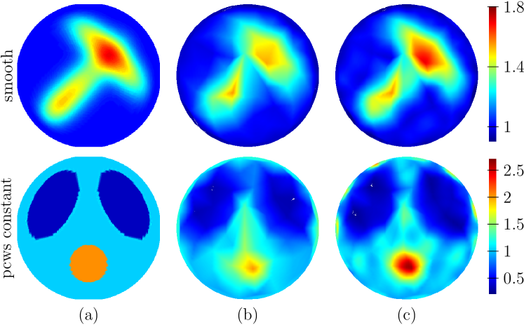
Figure 7: (a) True conductivity phantoms. (b) The output of the reconstruction mapping $\mathcal{Q}_{n}$, linearly interpolated on a grid obtained for layered media as in section 3.2.2. (c) One step of Gauss-Newton improves the reconstructions.

4.2.2 The optimal grids and sensitivity functions

The definition of the tensor product optimal grids considered in sections 2.2 and 3 does not extend to partial boundary measurement setups or to non-layered reference conductivity functions. We present here an alternative approach to determining the location of the points $P_{a,b}$ at which we approximate the conductivity in the output (4.4) of the reconstruction mapping. This approach extends to arbitrary setups, and it is based on the sensitivity analysis of the conductance function $\gamma$ to changes in the conductivity [16].

The sensitivity grid points are defined as the maxima of the sensitivity functions $D_{\sigma}\gamma_{a,b}({\bf x})$. They are the points at which the conductances $\gamma_{a,b}$ are most sensitive to changes in the conductivity. The sensitivity functions $D_{\sigma}\gamma({\bf x})$ are obtained by differentiating the identity $\Lambda_{\gamma(\sigma)}=\mathbf{M}_{n}(\Lambda_{\sigma})$ with respect to $\sigma$,

$$\left(D_{\sigma}\gamma\right)({\bf x})=\left(\left.D_{\gamma}{\bm{\Lambda}_{\gamma}}\right|_{{\bm{\Lambda}_{\gamma}}=\mathbf{M}_{n}(\Lambda_{\sigma})}\right)^{-1}\mathrm{vec}\left(\mathbf{M}_{n}(D\mathcal{K}_{\sigma})({\bf x})\right),\qquad{\bf x}\in\Omega.$$ (4.5)

The left hand side is a vector in $\mathbb{R}^{e}$. Its $k-$th entry is the Fréchet derivative of conductance $\gamma_{k}$ with respect to changes in the conductivity $\sigma$. The entries of the Jacobian $D_{\gamma}{\bm{\Lambda}_{\gamma}}\in\mathbb{R}^{e\times e}$ are

$$\left(D_{\gamma}{\bm{\Lambda}_{\gamma}}\right)_{jk}=\left(\mbox{vec}\left(\frac{\partial{\bm{\Lambda}_{\gamma}}}{\partial\gamma_{k}}\right)\right)_{j},$$ (4.6)

where $\mbox{vec}(A)$ denotes the operation of stacking in a vector in $\mathbb{R}^{e}$ the entries in the strict upper triangular part of a matrix $A\in\mathbb{R}^{n\times n}$. The last factor in (4.5) is the sensitivity of the measurements to changes of the conductivity, given by

$$\left(\mathbf{M}_{n}(D\mathcal{K}_{\sigma})\right)_{ij}({\bf x})=\left\{\begin{tabular}[]{ll}$\displaystyle\int\limits_{\mathcal{B}\times\mathcal{B}}\chi_{i}(x)D\mathcal{K}_{\sigma}({\bf x};x,y)\chi_{j}(y)dxdy$,&$i\neq j$,\\ \\ $-\displaystyle\sum\limits_{k\neq i}\int\limits_{\mathcal{B}\times\mathcal{B}}\chi_{i}(x)D\mathcal{K}_{\sigma}({\bf x};x,y)\chi_{k}(y)dxdy$,&$i=j$.\end{tabular}\right.$$ (4.7)

Here $\mathcal{K}_{\sigma}(x,y)$ is the kernel of the DtN map evaluated at points $x$ and $y\in\mathcal{B}$. Its Jacobian to changes in the conductivity is

$$D\mathcal{K}_{\sigma}({\bf x};x,y)=\sigma(x)\sigma(y)\left\{\nabla_{\bf x}({\bf n}(x)\cdot\nabla_{x}G(x,{\bf x}))\right\}\cdot\left\{\nabla_{\bf x}({\bf n}(y)\cdot\nabla_{y}G({\bf x},y))\right\},$$ (4.8)

where $G$ is the Green’s function of the differential operator $u\to\nabla\cdot(\sigma\nabla u)$ with Dirichlet boundary conditions, and ${\bf n}(x)$ is the outer unit normal at $x\in\mathcal{B}$. For more details on the calculation of the sensitivity functions see [16, Section 4].

$D_{\sigma}\gamma_{1,1/2}/\gamma_{1,1/2}^{(0)}$	$D_{\sigma}\gamma_{3/2,0}/\gamma_{3/2,0}^{(0)}$	$D_{\sigma}\gamma_{2,1/2}/\gamma_{2,1/2}^{(0)}$
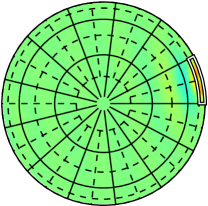
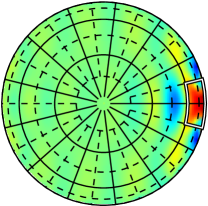
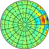
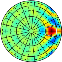
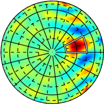
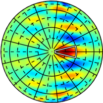
$D_{\sigma}\gamma_{5/2,0}/\gamma_{5/2,0}^{(0)}$	$D_{\sigma}\gamma_{3,1/2}/\gamma_{3,1/2}^{(0)}$	$D_{\sigma}\gamma_{7/2,0}/\gamma_{7/2,0}^{(0)}$

Figure 8: Sensitivity functions $\mbox{diag}\,(1/\gamma^{(0)})D_{\sigma}\gamma$ computed around the conductivity $\sigma=1$ for $n=13$. The images have a linear scale from dark blue to dark red spanning $\pm$ their maximum in absolute value. Light green corresponds to zero. We only display 6 sensitivity functions, the other ones can be obtained by integer multiple of $2\pi/13$ rotations. The primary grid is displayed in solid lines and the dual grid in dotted lines. The maxima of the sensitivity functions are very close to those of the optimal grid (intersection of solid and dotted lines).

The definition of the sensitivity grid points is

$$P_{a,b}=\arg\max_{{\bf x}\in\Omega}\,(D_{\sigma}\gamma_{{}_{a,b}})({\bf x}),\quad\mbox{evaluated at}~{}~{}\sigma=\sigma^{(o)}\equiv 1.$$ (4.9)

We display in Figure 8 the sensitivity functions with the superposed optimal grid obtained as in section 3.2.2. Note that the maxima of the sensitivity functions are very close to the optimal grid points in the full measurements case.

4.2.3 The preconditioned Gauss-Newton iteration

Since the reconstruction mapping $\mathcal{Q}_{n}$ gives good reconstructions when properly interpolated, we can think of it as an approximate inverse of the forward map $\mathbf{M}_{n}(\Lambda_{\sigma})$ and use it as a non-linear preconditioner. Instead of minimizing the misfit in the data, we solve the optimization problem

$$\min_{\sigma>0}\|\mathcal{Q}_{n}(\text{vec}\,(\mathbf{M}_{n}(\Lambda_{\sigma})))-\mathcal{Q}_{n}(\text{vec}\,(\mathbf{M}_{n}(\Lambda_{\sigma_{*}})))\|^{2}_{2}.$$ (4.10)

Here $\sigma_{*}$ is the conductivity that we would like to recover. For simplicity the minimization (4.10) is formulated with noiseless data and no regularization. We refer to [17] for a study of the effect of noise and regularization on the minimization (4.10).

The positivity constraints in (4.10) can be dealt with by solving for the log-conductivity $\kappa=\ln(\sigma)$ instead of the conductivity $\sigma$. With this change of variable, the residual in (4.10) can be minimized with the standard Gauss-Newton iteration, which we write in terms of the sensitivity functions (4.5) evaluated at $\sigma^{(j)}=\exp\kappa^{(j)}$:

$$\kappa^{(j+1)}=\kappa^{(j)}-\left(\mbox{diag}\,(1/\gamma^{(0)})\;D_{\sigma}\gamma\;\mbox{diag}\,(\exp\kappa^{(j)})\right)^{\dagger}\left[\mathcal{Q}_{n}(\text{vec}\,(\mathbf{M}_{n}(\Lambda_{\exp\kappa^{(j)}})))-\mathcal{Q}_{n}(\text{vec}\,(\mathbf{M}_{n}(\Lambda_{\sigma_{*}})))\right].$$ (4.11)

The superscript $\dagger$ denotes the Moore-Penrose pseudoinverse and the division is understood componentwise. We take as initial guess the log-conductivity $\kappa^{(0)}=\ln\sigma^{(0)}$, where $\sigma^{(0)}$ is given by the linear interpolation of $\mathcal{Q}_{n}(\text{vec}\,(\mathbf{M}_{n}(\Lambda_{\sigma_{*}}))$ on the optimal grid (i.e. the reconstruction from section 4.2.1). Having such a good initial guess helps with the convergence of the Gauss-Newton iteration. Our numerical experiments indicate that the residual in (4.10) is mostly reduced in the first iteration [13]. Subsequent iterations do not change significantly the reconstructions and result in negligible reductions of the residual in (4.10). Thus, for all practical purposes, the preconditioned problem is linear. We have also observed in [13, 17] that the conditioning of the linearized problem is significantly reduced by the preconditioner $\mathcal{Q}_{n}$.

Remark 6.

The conductivity obtained after one step of the Gauss-Newton iteration is in the span of the sensitivity functions (4.5). The use of the sensitivity functions as an optimal parametrization of the unknown conductivity was studied in [17]. Moreover, the same preconditioned Gauss-Newton idea was used in [37] for the inverse spectral problem of section 3.2.

We illustrate the improvement of the reconstructions with one Gauss-Newton step in Figure 7 (c). If prior information about the conductivity is available, it can be added in the form of a regularization term in (4.10). An example using total variation regularization is given in [13].

5 Two dimensional media and partial boundary measurements

In this section we consider the two dimensional EIT problem with partial boundary measurements. As mentioned in section 1, the boundary $\mathcal{B}$ is the union of the accessible subset $\mathcal{B}_{A}$ and the inaccessible subset $\mathcal{B}_{I}$. The accessible boundary $\mathcal{B}_{A}$ may consist of one or multiple connected components. We assume that the inaccessible boundary is grounded, so the partial boundary measurements are a set of Cauchy data $\left\{\left.u\right|_{{\mathcal{B}}_{A}},\left.\left(\sigma{\bf n}\cdot\nabla u\right)\right|_{{\mathcal{B}}_{A}}\right\}$, where $u$ satisfies (1.1) and $\left.u\right|_{{\mathcal{B}}_{I}}=0$. The inverse problem is to determine $\sigma$ from these Cauchy data.

Our inversion method described in the previous sections extends to the partial boundary measurement setup. But there is a significant difference concerning the definition of the optimal grids. The tensor product grids considered so far are essentially one dimensional, and they rely on the rotational invariance of the problem for $\sigma^{(o)}\equiv 1$. This invariance does not hold for the partial boundary measurements, so new ideas are needed to define the optimal grids. We present two approaches in sections 5.1 and 5.2. The first one uses circular planar networks with the same topology as before, and mappings that take uniformly distributed points on $\mathcal{B}$ to points on the accessible boundary $\mathcal{B}_{A}$. The second one uses networks with topologies designed specifically for the partial boundary measurement setups. The underlying two dimensional optimal grids are defined with sensitivity functions.

5.1 Coordinate transformations for the partial data problem

The idea of the approach described in this section is to map the partial data problem to one with full measurements at equidistant points, where we know from section 4 how to define the optimal grids. Since $\Omega$ is a unit disk, we can do this with diffeomorphisms of the unit disk to itself.

Let us denote such a diffeomorphism by $F$ and its inverse $F^{-1}$ by $G$. If the potential $u$ satisfies (1.1), then the transformed potential $\widetilde{u}(x)=u(F(x))$ solves the same equation with conductivity $\widetilde{\sigma}$ defined by

$$\widetilde{\sigma}(x)=\left.\frac{G^{\prime}(y)\sigma(y)\left(G^{\prime}(y)\right)^{T}}{\left|\det G^{\prime}(y)\right|}\right|_{y=F(x)},$$ (5.1)

where $G^{\prime}$ denotes the Jacobian of $G$. The conductivity $\widetilde{\sigma}$ is the push forward of $\sigma$ by $G$, and it is denoted by $G_{*}\sigma$. Note that if $G^{\prime}(y)\left(G^{\prime}(y)\right)^{T}\neq I$ and $\det G^{\prime}(y)\neq 0$, then $\widetilde{\sigma}$ is a symmetric positive definite tensor. If its eigenvalues are distinct, then the push forward of an isotropic conductivity is anisotropic.

The push forward $g_{*}\Lambda_{\sigma}$ of the DtN map is written in terms of the restrictions of diffeomorphisms $G$ and $F$ to the boundary. We call these restrictions $g=\left.G\right|_{\mathcal{B}}$ and $f=\left.F\right|_{\mathcal{B}}$ and write

$$((g_{*}\Lambda_{\sigma}){u_{{}_{\mathcal{B}}}})(\theta)=\left.(\Lambda_{\sigma}({u_{{}_{\mathcal{B}}}}\circ g))(\tau)\right|_{\tau=f(\theta)},\qquad\theta\in[0,2\pi),$$ (5.2)

for ${u_{{}_{\mathcal{B}}}}\in H^{1/2}(\mathcal{B})$. It is shown in [64] that the DtN map is invariant under the push forward in the following sense

$$g_{*}\Lambda_{\sigma}=\Lambda_{G_{*}\sigma}.$$ (5.3)

Therefore, given (5.3) we can compute the push forward of the DtN map, solve the inverse problem with data $g_{*}\Lambda_{\sigma}$ to obtain $G_{*}\sigma$, and then map it back using the inverse of (5.2). This requires the full knowledge of the DtN map. However, if we use the discrete analogue of the above procedure, we can transform the discrete measurements of $\Lambda_{\sigma}$ on $\mathcal{B}_{A}$ to discrete measurements at equidistant points on $\mathcal{B}$, from which we can estimate $\widetilde{\sigma}$ as described in section 4.

There is a major obstacle to this procedure: The EIT problem is uniquely solvable just for isotropic conductivities. Anisotropic conductivities are determined by the DtN map only up to a boundary-preserving diffeomorphism [64]. Two distinct approaches to overcome this obstacle are described in sections 5.1.1 and 5.1.2. The first one uses conformal mappings $F$ and $G$, which preserve the isotropy of the conductivity, at the expense of rigid placement of the measurement points. The second approach uses extremal quasiconformal mappings that minimize the artificial anisotropy of $\widetilde{\sigma}$ introduced by the placement at our will of the measurement points in $\mathcal{B}_{A}$.

5.1.1 Conformal mappings

The push forward $G_{*}\sigma$ of an isotropic $\sigma$ is isotropic if $G$ and $F$ satisfy $G^{\prime}\left((G^{\prime})^{T}\right)=I$ and $F^{\prime}\left((F^{\prime})^{T}\right)=I$. This means that the diffeomorphism is conformal and the push forward is simply

$$G_{*}\sigma=\sigma\circ F.$$ (5.4)

Since all conformal mappings of the unit disk to itself belong to the family of Möbius transforms [48], $F$ must be of the form

$$F(z)=e^{i\omega}\frac{z-a}{1-\overline{a}z},\qquad z\in\mathbb{C},~{}~{}|z|\leq 1,~{}~{}\omega\in[0,2\pi),~{}~{}a\in\mathbb{C},~{}~{}|a|<1,$$ (5.5)

where we associate $\mathbb{R}^{2}$ with the complex plane $\mathbb{C}$. Note that the group of transformations (5.5) is extremely rigid, its only degrees of freedom being the numerical parameters $a$ and $\omega$.

To use the full data discrete inversion procedure from section 4 we require that $G$ maps the accessible boundary segment $\mathcal{B}_{A}=\left\{e^{i\tau}\;|\;\tau\in[-\beta,\beta]\right\}$ to the whole boundary with the exception of one segment between the equidistant measurement points $\theta_{k}$, $k=(n+1)/2,\;(n+3)/2$ as shown in Figure 9. This determines completely the values of the parameters $a$ and $\omega$ in (5.5) which in turn determine the mapping $f$ on the boundary. Thus, we have no further control over the positioning of the measurement points $\tau_{k}=f(\theta_{k})$, $k=1,\ldots,n$.

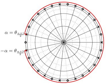
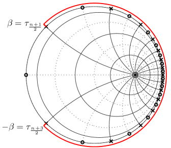
Figure 9: The optimal grid in the unit disk (left) and its image under the conformal mapping $F$ (right). Primary grid lines are solid black, dual grid lines are dotted black. Boundary grid nodes: primary $\times$, dual $\circ$. The accessible boundary segment $\mathcal{B}_{A}$ is shown in solid red.

As shown in Figure 9 the lack of control over $\tau_{k}$ leads to a grid that is highly non-uniform in angle. In fact it is demonstrated in [15] that as $n$ increases there is no asymptotic refinement of the grid away from the center of $\mathcal{B}_{A}$, where the points accumulate. However, since the limit $n\to\infty$ is unattainable in practice due to the severe ill-conditioning of the problem, the grids obtained by conformal mapping can still be useful in practical inversion. We show reconstructions with these grids in section 5.3.

5.1.2 Extremal quasiconformal mappings

To overcome the issues with conformal mappings that arise due to the inherent rigidity of the group of conformal automorphisms of the unit disk, we use here quasiconformal mappings. A quasiconformal mapping $F$ obeys a Beltrami equation in $\Omega$

$$\frac{\partial F}{\partial\overline{z}}=\mu(z)\frac{\partial F}{\partial z},\quad\|\mu\|_{\infty}<1,$$ (5.6)

with a Beltrami coefficient $\mu(z)$ that measures how much $F$ differs from a conformal mapping. If $\mu\equiv 0$, then (5.6) reduces to the Cauchy-Riemann equation and $F$ is conformal. The magnitude of $\mu$ also provides a measure of the anisotropy $\kappa$ of the push forward of $\sigma$ by $F$. The definition of the anisotropy is

$$\kappa(F_{*}\sigma,z)=\frac{\sqrt{\lambda_{1}(z)/\lambda_{2}(z)}-1}{\sqrt{\lambda_{1}(z)/\lambda_{2}(z)}+1},$$ (5.7)

where $\lambda_{1}(z)$, $\lambda_{2}(z)$ are the largest and the smallest eigenvalues of $F_{*}\sigma$ respectively. The connection between $\mu$ and $\kappa$ is given by

$$\kappa\left(F_{*}\sigma,z\right)=|\mu(z)|,$$ (5.8)

and the maximum anisotropy is

$$\kappa(F_{*}\sigma)=\sup_{z}\kappa(F_{*}\sigma,z)=\|\mu\|_{\infty}.$$ (5.9)

Since the unknown conductivity is isotropic, we would like to minimize the amount of artificial anisotropy that we introduce into the reconstruction by using $F$. This can be done with extremal quasiconformal mappings, which minimize $\|\mu\|_{\infty}$ under constraints that fix $f=\left.F\right|_{\mathcal{B}}$, thus allowing us to control the positioning of the measurement points $\tau_{k}=f(\theta_{k})$, for $k=1,\ldots,n$.

For sufficiently regular boundary values $f$ there exists a unique extremal quasiconformal mapping that is known to be of a Teichmüller type [63]. Its Beltrami coefficient satisfies

$$\mu(z)=\|\mu\|_{\infty}\frac{\overline{\phi(z)}}{|\phi(z)|},$$ (5.10)

for some holomorphic function $\phi(z)$ in $\Omega$. Similarly, we can define the Beltrami coefficient for $G$, using a holomorphic function $\psi$. It is established in [62] that $F$ admits a decomposition

$$F=\Psi^{-1}\circ A_{K}\circ\Phi,$$ (5.11)

where

$$\Phi(z)=\int\sqrt{\phi(z)}dz,\qquad\Psi(\zeta)=\int\sqrt{\psi(\zeta)}d\zeta,$$ (5.12)

are conformal away from the zeros of $\phi$ and $\psi$, and

$$A_{K}(x+iy)=Kx+iy$$ (5.13)

is an affine stretch, the only source of anisotropy in (5.11):

$$\kappa\left(F_{*}\sigma\right)=\|\mu\|_{\infty}=\left|\frac{K-1}{K+1}\right|.$$ (5.14)

Since only the behavior of $f$ at the measurement points $\theta_{k}$ is of interest to us, it is possible to construct explicitly the mappings $\Phi$ and $\Psi$ [15]. They are Schwartz-Christoffel conformal mappings of the unit disk to polygons of special form, as shown in Figure 10. See [15, Section 3.4] for more details.

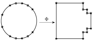
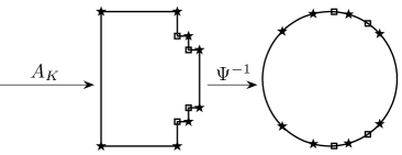
Figure 10: Teichmüller mapping decomposed into conformal mappings $\Phi$ and $\Psi$, and an affine transform $A_{K}$. The poles of $\phi$ and $\psi$ and their images under $\Phi$ and $\Psi$ are $\bigstar$, the zeros of $\phi$ and $\psi$ and their images under $\Phi$ and $\Psi$ are $\square$.

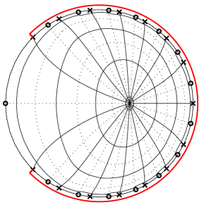
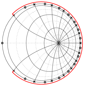
Figure 11: The optimal grid under the quasiconformal Teichmüller mappings $F$ with different $K$. Left: $K=0.8$ (smaller anisotropy); right: $K=0.66$ (higher anisotropy). Primary grid lines are solid black, dual grid lines are dotted black. Boundary grid nodes: primary $\times$, dual $\circ$. The accessible boundary segment $\mathcal{B}_{A}$ is shown in solid red.

We demonstrate the behavior of the optimal grids under the extremal quasiconformal mappings in Figure 11. We present the results for two different values of the affine stretching constant $K$. As we increase the amount of anisotropy from $K=0.8$ to $K=0.66$, the distribution of the grid nodes becomes more uniform. The price to pay for this more uniform grid is an increased amount of artificial anisotropy, which may detriment the quality of the reconstruction, as shown in the numerical examples in section 5.3.

5.2 Special network topologies for the partial data problem

The limitations of the construction of the optimal grids with coordinate transformations can be attributed to the fact that there is no non-singular mapping between the full boundary $\mathcal{B}$ and its proper subset $\mathcal{B}_{A}$. Here we describe an alternative approach, that avoids these limitations by considering networks with different topologies, constructed specifically for the partial measurement setups. The one-sided case, with the accessible boundary $\mathcal{B}_{A}$ consisting of one connected segment, is in section 5.2.1. The two sided case, with $\mathcal{B}_{A}$ the union of two disjoint segments, is in section 5.2.2. The optimal grids are constructed using the sensitivity analysis of the discrete and continuum problems, as explained in sections 4.2.2 and 5.2.3.

5.2.1 Pyramidal networks for the one-sided problem

We consider here the case of $\mathcal{B}_{A}$ consisting of one connected segment of the boundary. The goal is to choose a topology of the resistor network based on the flow properties of the continuum partial data problem. Explicitly, we observe that since the potential excitation is supported on $\mathcal{B}_{A}$, the resulting currents should not penetrate deep into $\Omega$, away from $\mathcal{B}_{A}$. The currents are so small sufficiently far away from $\mathcal{B}_{A}$ that in the discrete (network) setting we can ask that there is no flow escaping the associated nodes. Therefore, these nodes are interior ones. A suitable choice of networks that satisfy such conditions was proposed in [16]. We call them pyramidal and denote their graphs by $\Gamma_{n}$, with $n$ the number of boundary nodes.

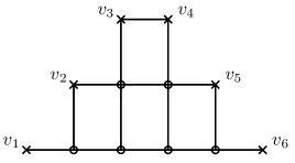
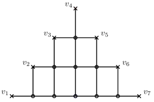
Figure 12: Pyramidal networks $\Gamma_{n}$ for $n=6$, $7$. The boundary nodes $v_{j}$, $j=1,\ldots,n$ are indicated with $\times$ and the interior nodes with $\circ$.

We illustrate two pyramidal graphs in Figure 12, for $n=6$ and $7$. Note that it is not necessary that $n$ be odd for the pyramidal graphs $\Gamma_{n}$ to be critical, as was the case in the previous sections. In what follows we refer to the edges of $\Gamma_{n}$ as vertical or horizontal according to their orientation in Figure 12. Unlike the circular networks in which all the boundary nodes are in a sense adjacent, there is a gap between the boundary nodes $v_{1}$ and $v_{n}$ of a pyramidal network. This gap is formed by the bottommost $n-2$ interior nodes that enforce the condition of zero normal flux, the approximation of the lack of penetration of currents away from $\mathcal{B}_{A}$.

It is known from [23, 16] that the pyramidal networks are critical and thus uniquely recoverable from the DtN map. Similar to the circular network case, pyramidal networks can be recovered using a layer peeling algorithm in a finite number of algebraic operations. We recall such an algorithm below, from [16], in the case of even $n=2m$. A similar procedure can also be used for odd $n$.

Algorithm 1.

To determine the conductance $\gamma$ of the pyramidal network $\left(\Gamma_{n},\gamma\right)$ from the DtN map $\bm{\Lambda}^{(n)}$, perform the following steps:

$Z=\{v_{1},\ldots,v_{p-1},v_{p+1},\ldots,v_{m}\}$, $C=\{v_{m+2},\ldots,v_{2m}\}$, $H=\{v_{1},\ldots,v_{p}\}$ and $V=\{v_{p},\ldots,v_{m+1}\}$, in the case $p\leq m$. $Z=\{v_{m+1},\ldots,v_{p-1},v_{p+1},\ldots,v_{2m}\}$, $C=\{v_{1},\ldots,v_{m-1}\}$, $H=\{v_{p},\ldots,v_{2m}\}$ and $V=\{v_{m},\ldots,v_{p}\}$, for $m+1\leq p\leq 2m$. (2) Compute the conductance $\gamma(E_{p,h})$ of the horizontal edge emanating from $v_{p}$ using $$\gamma(E_{p,h})=\left(\bm{\Lambda}^{(n)}_{p,H}-\bm{\Lambda}^{(n)}_{p,C}\;\left(\bm{\Lambda}^{(n)}_{Z,C}\right)^{-1}\;\bm{\Lambda}^{(n)}_{Z,H}\right){\bf 1}_{H},$$ (5.15) compute the conductance $\gamma(E_{p,v})$ of the vertical edge emanating from $v_{p}$ using $$\gamma(E_{p,v})=\left(\bm{\Lambda}^{(n)}_{p,V}-\bm{\Lambda}^{(n)}_{p,C}\;\left(\bm{\Lambda}^{(n)}_{Z,C}\right)^{-1}\;\bm{\Lambda}^{(n)}_{Z,V}\right){\bf 1}_{V},$$ (5.16) where ${\bf 1}_{V}$ and ${\bf 1}_{H}$ are column vectors of all ones. (3) Once $\gamma(E_{p,h})$, $\gamma(E_{p,v})$ are known, peel the outer layer from $\Gamma_{n}$ to obtain the subgraph $\Gamma_{n-2}$ with the set $\mathcal{S}=\{w_{1},\ldots,w_{2m-2}\}$ of boundary nodes. Assemble the blocks ${\bf K}_{\mathcal{SS}}$, ${\bf K}_{\mathcal{SB}}$, ${\bf K}_{\mathcal{BS}}$, ${\bf K}_{\mathcal{BB}}$ of the Kirchhoff matrix of $(\Gamma_{n},\gamma)$, and compute the updated DtN map $\bm{\Lambda}^{(n-2)}$ of the smaller network $(\Gamma_{n-2},\gamma)$, as follows $$\bm{\Lambda}^{(n-2)}=-{\bf K}_{\mathcal{SS}}^{\prime}-{\bf K}_{\mathcal{SB}}\;{\bf P}^{T}\;\left({\bf P}\;(\bm{\Lambda}^{(n)}-{\bf K}_{\mathcal{BB}})\;{\bf P}^{T}\right)^{-1}\;{\bf P}\;{\bf K}_{\mathcal{BS}}.$$ (5.17) Here ${\bf P}\in\mathbb{R}^{(n-2)\times n}$ is a projection operator: ${\bf P}{\bf P}^{T}={\bf I}_{n-2}$, and ${\bf K}_{\mathcal{SS}}^{\prime}$ is a part of ${\bf K}_{\mathcal{SS}}$ that only includes the contributions from the edges connecting $\mathcal{S}$ to $\mathcal{B}$. (4) If $m=1$ terminate. Otherwise, decrease $m$ by 1, update $n=2m$ and go back to step 1. Similar to the layer peeling method in [22], Algorithm 1 is based on the construction of special solutions. In steps 1 and 2 the special solutions are constructed implicitly, to enforce a unit potential drop on edges $E_{p,h}$ and $E_{p,v}$ emanating from the boundary node $v_{p}$. Since the DtN map is known, so is the current at $v_{p}$, which equals to the conductance of an edge due to a unit potential drop on that edge. Once the conductances are determined for all the edges adjacent to the boundary, the layer of edges is peeled off and the DtN map of a smaller network $\Gamma_{n-2}$ is computed in step 3. After $m$ layers have been peeled off, the network is completely recovered. The algorithm is studied in detail in [16], where it is also shown that all matrices that are inverted in (5.15), (5.16) and (5.17) are non-singular.

Remark 7.

The DtN update formula (5.17) provides an interesting connection to the layered case. It can be viewed as a matrix generalization of the continued fraction representation (3.36). The difference between the two formulas is that (3.36) expresses the eigenvalues of the DtN map, while (5.17) gives an expression for the DtN map itself.

5.2.2 The two-sided problem

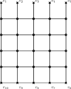
Figure 13: Two-sided network $T_{n}$ for $n=10$. Boundary nodes $v_{j}$, $j=1,\ldots,n$ are $\times$, interior nodes are $\circ$.

We call the problem two-sided when the accessible boundary $\mathcal{B}_{A}$ consists of two disjoint segments of $\mathcal{B}$. A suitable network topology for this setting was introduced in [17]. We call these networks two-sided and denote their graphs by $T_{n}$, with $n$ the number of boundary nodes assumed even $n=2m$. Half of the nodes are on one segment of the boundary and the other half on the other, as illustrated in Figure 13. Similar to the one-sided case, the two groups of $m$ boundary nodes are separated by the outermost interior nodes, which model the lack of penetration of currents away from the accessible boundary segments. One can verify that the two-sided network is critical, and thus it can be uniquely recovered from the DtN map by the Algorithm 2 introduced in [17].

When referring to either the horizontal or vertical edges of a two sided network, we use their orientation in Figure 13.

Algorithm 2.

To determine the conductance $\gamma$ of the two-sided network $(T_{n},\gamma)$ from the DtN map $\bm{\Lambda}_{\gamma}$, perform the following steps:

For $p=m+2,m+3,\ldots,2m$ define the sets $Z=\{p+1,p+2,\ldots,p+m-1\}$ and $C=\{p-2,p-3,\ldots,p-m\}$. The conductance of the edge $E_{p,q,h}$ between $v_{p}$ and $v_{q}$, $q=p-1$ is given by

$$\gamma(E_{p,q,h})=-\bm{\Lambda}_{p,q}+\bm{\Lambda}_{p,C}(\bm{\Lambda}_{Z,C})^{-1}\bm{\Lambda}_{Z,q}.$$ (5.18)

Assemble a symmetric tridiagonal matrix $\bm{A}$ with off-diagonal entries $-\gamma(E_{p,p-1,h})$ and rows summing to zero. Update the lower right $m$-by-$m$ block of the DtN map by subtracting $\bm{A}$ from it. (2) Let $s=m-1$. (3) Peel the top and bottom layers of vertical resistors: For $p=1,2,\ldots,2m$ define the sets $L=\{p-1,p-2,\ldots,p-s\}$ and $R=\{p+1,p+2,\ldots,p+s\}$. If $p<m/2$ for the top layer, or $p>3m/2$ for the bottom layer, set $Z=L$, $C=R$. Otherwise let $Z=R$, $C=L$. The conductance of the vertical edge emanating from $v_{p}$ is given by $$\gamma(E_{p,v})=\bm{\Lambda}_{p,p}-\bm{\Lambda}_{p,C}(\bm{\Lambda}_{Z,C})^{-1}\bm{\Lambda}_{Z,p}.$$ (5.19) Let $\bm{D}=\mbox{diag}\left(\gamma(E_{p,v})\right)$ and update the DtN map $$\bm{\Lambda}_{\gamma}=-\bm{D}-\bm{D}\left(\bm{\Lambda}_{\gamma}+\bm{D}\right)^{-1}\bm{D}.$$ (5.20) (4) If $s=1$ go to step (7). Otherwise decrease $s$ by $2$. (5) Peel the top and bottom layers of horizontal resistors: For $p=1,2,\ldots,2m$ define the sets $L=\{p-1,p-2,\ldots,p-s\}$ and $R=\{p+2,p+3,\ldots,p+s+1\}$. If $p<m/2$ for the top layer, or $p<3m/2$ for the bottom layer, set $Z=L$, $C=R$, $q=p+1$. Otherwise let $Z=R$, $C=L$, $q=p-1$. The conductance of the edge connecting $v_{p}$ and $v_{q}$ is given by (5.18). Update the upper left and lower right blocks of the DtN map as in step (1). (6) If $s=0$ go to step (7), otherwise go to (3). (7) Determine the last layer of resistors. If $m$ is odd the remaining vertical resistors are the diagonal entries of the DtN map. If $m$ is even, the remaining resistors are horizontal. The leftmost of the remaining horizontal resistors $\gamma(E_{1,2,h})$ is determined from (5.18) with $p=1$, $q=m+1$, $C=\{1,2\}$, $Z=\{m+1,m+2\}$ and a change of sign. The rest are determined by $$\gamma(E_{p,p+1,h})=\left(\bm{\Lambda}_{p,H}-\bm{\Lambda}_{p,C}(\bm{\Lambda}_{Z,C})^{-1}\bm{\Lambda}_{Z,H}\right)\mathbf{1},$$ (5.21) where $p=2,3,\ldots,m-1$, $C=\{p-1,p,p+1\}$, $Z=\{p+m-1,p+m,p+m+1\}$, $H=\{p+m-1,p+m\}$, and $\mathbf{1}$ is a vector $(1,1)^{T}$. Similar to Algorithm 1, Algorithm 2 is based on the construction of special solutions examined in [22, 24]. These solutions are designed to localize the flow on the outermost edges, whose conductance we determine first. In particular, formulas (5.18) and (5.19) are known as the “boundary edge” and “boundary spike” formulas [24, Corollaries 3.15 and 3.16].

5.2.3 Sensitivity grids for pyramidal and two-sided networks

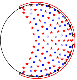
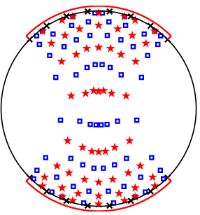
Figure 14: Sensitivity optimal grids in the unit disk for the pyramidal network $\Gamma_{n}$ (left) and the two-sided network $T_{n}$ (right) with $n=16$. The accessible boundary segments $\mathcal{B}_{A}$ are solid red. Blue $\square$ correspond to vertical edges, red $\bigstar$ correspond to horizontal edges, measurement points are black $\times$.

The underlying grids of the pyramidal and two-sided networks are truly two dimensional, and they cannot be constructed explicitly as in section 3 by reducing the problem to a one dimensional one. We define the grids with the sensitivity function approach described in section 4.2.2. The computed sensitivity grid points are presented in Figure 14, and we observe a few important properties. First, the neighboring points corresponding to the same type of resistors (vertical or horizontal) form rather regular virtual quadrilaterals. Second, the points corresponding to different types of resistors interlace in the sense of lying inside the virtual quadrilaterals formed by the neighboring points of the other type. Finally, while there is some refinement near the accessible boundary (more pronounced in the two-sided case), the grids remain quite uniform throughout the covered portion of the domain.

Note from Figure 13 that the graph $T_{n}$ lacks the upside-down symmetry. Thus, it is possible to come up with two sets of optimal grid nodes, by fitting the measured DtN map $\mathbf{M}_{n}(\Lambda_{\sigma})$ once with a two-sided network and the second time with the network turned upside-down. This way the number of nodes in the grid is essentially doubled, thus doubling the resolution of the reconstruction. However, this approach can only improve resolution in the direction transversal to the depth, as shown in [17, Section 2.5].

5.3 Numerical results

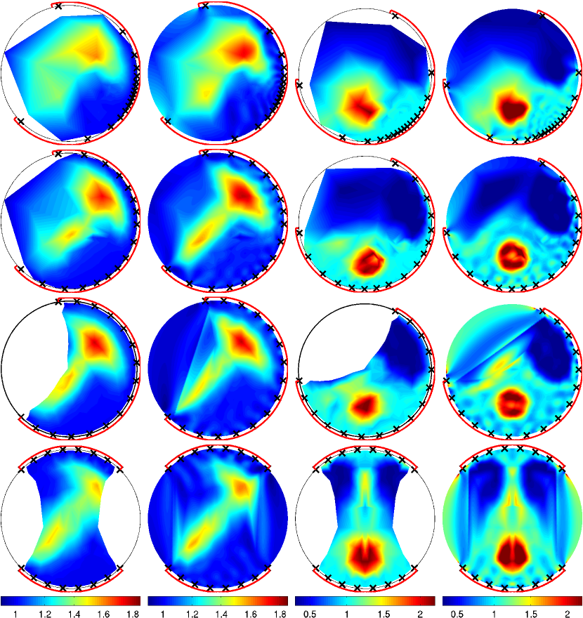
Figure 15: Reconstructions with partial data. Same conductivities are used as in figure 7. Two leftmost columns: smooth conductivity. Two rightmost columns: piecewise constant chest phantom. Columns 1 and 3: piecewise linear reconstructions. Columns 2 and 4: reconstructions after one step of Gauss-Newton iteration (4.11). Rows from top to bottom: conformal mapping, quasiconformal mapping, pyramidal network, two-sided network. Accessible boundary $\mathcal{B}_{A}$ is solid red. Centers of supports of measurement (electrode) functions $\chi_{q}$ are $\times$.

We present in this section numerical reconstructions with partial boundary measurements. The reconstructions with the four methods from sections 5.1.1, 5.1.2, 5.2.1 and 5.2.2 are compared row by row in Figure 15. We use the same two test conductivities as in Figure 7(a). Each row in Figure 15 corresponds to one method. For each test conductivity, we show first the piecewise linear interpolation of the entries returned by the reconstruction mapping $\mathcal{Q}_{n}$, on the optimal grids (first and third column in Figure 15). Since these grids do not cover the entire $\Omega$, we display the results only in the subset of $\Omega$ populated by the grid points. We also show the reconstructions after one-step of the Gauss-Newton iteration (4.11) (second and fourth columns in Figure 15).

As expected, the reconstructions with the conformal mapping grids are the worst. The highly non-uniform conformal mapping grids cannot capture the details of the conductivities away from the middle of the accessible boundary. The reconstructions with quasiconformal grids perform much better, capturing the details of the conductivities much more uniformly throughout the domain. Although the piecewise linear reconstructions $\mathcal{Q}_{n}$ have slight distortions in the geometry, these distortions are later removed by the first step of the Gauss-Newton iteration. The piecewise linear reconstructions with pyramidal and two-sided networks avoid the geometrical distortions of the quasiconformal case, but they are also improved after one step of the Gauss-Newton iteration.

Note that while the Gauss-Newton step improves the geometry of the reconstructions, it also introduces some spurious oscillations. This is more pronounced for the piecewise constant conductivity phantom (fourth column in Figure 15). To overcome this problem one may consider regularizing the Gauss-Newton iteration (4.11) by adding a penalty term of some sort. For example, for the piecewise constant phantom, we could penalize the total variation of the reconstruction, as was done in [13].

6 Summary

We presented a discrete approach to the numerical solution of the inverse problem of electrical impedance tomography (EIT) in two dimensions. Due to the severe ill-posedness of the problem, it is desirable to parametrize the unknown conductivity $\sigma({\bf x})$ with as few parameters as possible, while still capturing the best attainable resolution of the reconstruction. To obtain such a parametrization, we used a discrete, model reduction formulation of the problem. The discrete models are resistor networks with special graphs.

We described in detail the solvability of the model reduction problem. First, we showed that boundary measurements of the continuum Dirichlet to Neumann (DtN) map $\Lambda_{\sigma}$ for the unknown $\sigma({\bf x})$ define matrices that belong to the set of discrete DtN maps for resistor networks. Second, we described the types of network graphs appropriate for different measurement setups. By appropriate we mean those graphs that ensure unique recoverability of the network from its DtN map. Third, we showed how to determine the networks.

We established that the key ingredient in the connection between the discrete model reduction problem (inverse problem for the network) and the continuum EIT problem is the optimal grid. The name optimal refers to the fact that finite volumes discretizations on these grids give spectrally accurate approximations of the DtN map, the data in EIT. We defined reconstructions of the conductivity using the optimal grids, and studied them in detail in three cases: (1) The case of layered media and full boundary measurements, where the problem can be reduced to one dimension via Fourier transforms. (2) The case of two dimensional media with measurement access to the entire boundary. (3) The case of two dimensional media with access to a subset of the boundary.

We presented the available theory behind our inversion approach and illustrated its performance with numerical simulations.

Acknowledgements

The work of L. Borcea was partially supported by the National Science Foundation grants DMS-0934594, DMS-0907746 and by the Office of Naval Research grant N000140910290. The work of F. Guevara Vasquez was partially supported by the National Science Foundation grant DMS-0934664. The work of A.V. Mamonov was partially supported by the National Science Foundation grants DMS-0914465 and DMS-0914840. LB, FGV and AVM were also partially supported by the National Science Foundation and the National Security Agency, during the Fall 2010 special semester on Inverse Problems at MSRI, Berkeley, CA.

Appendix A The quadrature formulas

To understand definitions (3.8), recall Figure 1. Take for example the dual edge

$$\Sigma_{i-\frac{1}{2},j}=(P_{i-\frac{1}{2},j-\frac{1}{2}},P_{i-\frac{1}{2},j-\frac{1}{2}}),$$

where $P_{i-\frac{1}{2},j-\frac{1}{2}}=\widehat{r}_{i}(\cos\widehat{\theta}_{j},\sin\widehat{\theta}_{j})$. We have from (2.5), and the change of variables to $z(r)$ that

$$\int_{\Sigma_{i-\frac{1}{2},j}}\sigma({\bf x}){\bf n}({\bf x})\cdot\nabla u({\bf x})ds({\bf x})=\int_{\widehat{\theta}_{j}}^{\widehat{\theta}_{j+1}}\widehat{r}_{i-1}\sigma(\widehat{r}_{i-1})\frac{\partial u(\widehat{r}_{i-1},\theta)}{\partial r}d\theta\approx-h_{\theta}\frac{\partial u(\widehat{r}_{i-1},\theta_{j})}{\partial z}\approx\frac{h_{\theta}\left(U_{i-1,j}-U_{i,j}\right)}{z(r_{i})-z(r_{i-1})},$$

which gives the first equation in (3.8). Similarly, the flux across

$$\Sigma_{i,j+\frac{1}{2}}=(P_{i-\frac{1}{2},j+\frac{1}{2}},P_{i+\frac{1}{2},j+\frac{1}{2}}),$$

is given by

$$\int_{\Sigma_{i,j+\frac{1}{2}}}\sigma({\bf x}){\bf n}({\bf x})\cdot\nabla u({\bf x})ds({\bf x}) = \int_{\widehat{r}_{i}}^{\widehat{r}_{i-1}}\frac{\sigma(r)}{r}\frac{\partial u(r,\widehat{\theta}_{j+1})}{\partial\theta}dr\approx\frac{\partial u(r_{i},\widehat{\theta}_{j+1})}{\partial\theta}\int_{\widehat{r}_{i}}^{\widehat{r}_{i-1}}\frac{\sigma(r)}{r}dr$$

$$\approx \left(\widehat{z}(\widehat{r}_{i})-\widehat{z}(\widehat{r}_{i-1})\right)\frac{U_{i,j+1}-U(i,j)}{h_{\theta}},$$

which gives the second equation in (3.8).

Appendix B Continued fraction representation

Let us begin with the system of equations satisfied by the potential $V_{j}$, which we rewrite as

$$b_{j} = b_{j+1}+\widehat{\alpha}_{j+1}\lambda V_{j+1},\qquad j=0,1,\ldots\ell,$$

$$b_{0} = \Phi_{{}_{\mathcal{B}}},$$ (2.1)

$$V_{\ell+1} = 0,$$

where we let

$$V_{j}=V_{j+1}+\alpha_{j}b_{j}.$$ (2.2)

Combining the first equation in (2.2) with (2.2), we obtain the recursive relation

$$\frac{b_{j}}{V_{j}}=\cfrac{1}{\alpha_{j}+\cfrac{1}{\widehat{\alpha}_{j+1}\lambda+\cfrac{b_{j+1}}{V_{j+1}}}},\qquad j=1,2,\ldots,\ell,$$ (2.3)

which we iterate for $j$ decreasing from $j=\ell-1$ to $1$, and starting with

$$\frac{b_{\ell}}{V_{\ell}}=\frac{1}{\alpha_{\ell}}.$$ (2.4)

The latter follows from the first equation in (2.1) evaluated at $j=\ell$, and boundary condition $V_{\ell+1}=0$. We obtain that

$$F^{\dagger}(\lambda)=V_{1}/\Phi_{{}_{\mathcal{B}}}=\frac{V_{1}}{b_{0}}=\cfrac{V_{1}}{b_{1}+\widehat{\alpha}_{1}\lambda V_{1}}=\cfrac{1}{\widehat{\alpha}_{1}\lambda+\cfrac{b_{1}}{V_{1}}}$$ (2.5)

has the continued fraction representation (3.36).

Appendix C Derivation of results (3.47-3.48)

To derive equation (3.47) let us begin with the Fourier series of the electrode functions

$$\chi_{q}(\theta)=\sum_{k\in\mathbb{Z}}C_{q}(k)e^{ik\theta}=\sum_{k\in\mathbb{Z}}\overline{C_{q}(k)}e^{-ik\theta},$$ (3.6)

where the bar denotes complex conjugate and the coefficients are

$$C_{q}(\theta)=\frac{1}{2\pi}\int_{0}^{2\pi}\chi_{q}(\theta)e^{ik\theta}d\theta=\frac{e^{ik\theta_{q}}}{2\pi}\mbox{sinc}\left(\frac{kh_{\theta}}{2}\right).$$ (3.7)

Then, we have

$$\left({\bm{\Lambda}_{\gamma}}\right)_{p,q} = \int_{0}^{2\pi}\chi_{p}(\theta)\Lambda_{\sigma}\chi_{q}(\theta)d\theta=\sum_{k,k^{\prime}\in\mathbb{Z}}C_{p}(k)\overline{C_{q}(k^{\prime})}\int_{0}^{2\pi}e^{ik\theta}\Lambda_{\sigma}e^{-ik^{\prime}\theta}d\theta$$ (3.8)

$$= \frac{1}{2\pi}\sum_{k\in\mathbb{Z}}e^{ik(\theta_{p}-\theta_{q})}f(k^{2})\left[\mbox{sinc}\left(\frac{kh_{\theta}}{2}\right)\right]^{2},\qquad p\neq q.$$

The diagonal entries are

$$\left({\bm{\Lambda}_{\gamma}}\right)_{p,p}=-\sum_{q\neq p}\left({\bm{\Lambda}_{\gamma}}\right)_{p,q}=-\frac{1}{2\pi}\sum_{k\in\mathbb{Z}}e^{ik\theta_{p}}f(k^{2})\left[\mbox{sinc}\left(\frac{kh_{\theta}}{2}\right)\right]^{2}\sum_{q\neq p}e^{-ik\theta_{q}}.$$ (3.9)

But

$$\sum_{q\neq p}e^{-ik\theta_{q}}=\sum_{q=1}^{n}e^{-i\frac{2\pi k}{n}(q-1)}-e^{-ik\theta_{p}}=e^{i\pi k(1-1/n)}\frac{\sin(\pi k)}{\sin(\pi k/n)}-e^{-ik\theta_{p}}=n\delta_{k,0}-e^{ik\theta_{p}}.$$ (3.10)

Since $f(0)=0$, we obtain from (3.9-3.12) that (3.8) holds for $p=q$, as well. This is the result (3.47). Moreover, (3.48) follows from

$$\left({\bm{\Lambda}_{\gamma}}\left[e^{ik\theta}\right]\right)_{p}=\sum_{q=1}^{n}\left({\bm{\Lambda}_{\gamma}}\right)_{p,q}e^{ik\theta_{q}}=\frac{1}{2\pi}\sum_{k_{1}\in\mathbb{Z}}e^{ik_{1}\theta_{p}}f(k_{1}^{2})\left[\mbox{sinc}\left(\frac{k_{1}h_{\theta}}{2}\right)\right]^{2}\sum_{q=1}^{n}e^{i(k-k_{1})\theta_{q}},$$ (3.11)

and the identity

$$\sum_{q=1}^{n}e^{i(k-k_{1})\theta_{q}}=\sum_{q=1}^{n}e^{i\frac{2\pi(k-k_{1})}{n}(q-1)}=n\delta_{k,k_{1}}.$$ (3.12)

Appendix D Rational interpolation and Euclidean division

Consider the case $m_{1/2}=1$, where $F(\lambda)=1/F^{\dagger}(\lambda)$ follows from (3.36). We rename the coefficients as

$$\kappa_{2j-1}=\widehat{\alpha}_{j},\quad\kappa_{2j}=\alpha_{j},\quad j=1,\ldots\ell,$$ (4.13)

and let $\lambda=x^{2}$ to obtain

$$\frac{F(x^{2})}{x}=\kappa_{1}x+\cfrac{1}{\kappa_{2}x+\dots\cfrac{1}{\kappa_{2\ell-1}x+\cfrac{1}{\kappa_{2\ell}x}}}.$$ (4.14)

To determine $\kappa_{j}$, for $j=1,\ldots,2\ell$, we write first (4.14) as the ratio of two polynomials of $x$, $P_{2\ell}(x)$ and $Q_{2\ell-1}(x)$ of degrees $2\ell$ and $2\ell-1$ respectively, and seek their coefficients $c_{j}$,

$$\frac{F(x^{2})}{x}=\frac{P_{2\ell}(x)}{Q_{2\ell-1}(x)}=\frac{c_{2\ell}x^{2\ell}+c_{2(\ell-1)}x^{2(\ell-1)}+\ldots+c_{2}x^{2}+c_{0}}{c_{2\ell-1}x^{2\ell-1}+c_{2\ell-3}x^{2\ell-3}+\ldots+c_{1}x}.$$ (4.15)

We normalize the ratio by setting $c_{0}=-1$.

Now suppose that we have measurements of $F$ at $\lambda_{k}=x_{k}^{2}$, for $k=1,\ldots,2\ell$, and introduce the notation

$$\frac{F(x_{k}^{2})}{x_{k}}=D_{k}.$$ (4.16)

We obtain from (4.15) the following linear system of equations for the coefficients

$$P_{2\ell}(x_{k})-D_{k}Q_{2\ell-1}(x_{k})=0,\qquad k=1,\ldots,2\ell,$$ (4.17)

or in matrix form

$$\left(\begin{array}[]{cccccc}-D_{1}x_{1}&x_{1}^{2}&-D_{1}x_{1}^{3}&\ldots&-D_{1}x_{1}^{2\ell-1}&x_{1}^{2\ell}\\ -D_{2}x_{2}&x_{2}^{2}&-D_{2}x_{2}^{3}&\ldots&-D_{2}x_{2}^{2\ell-1}&x_{2}^{2\ell}\\ &&&\vdots\\ -D_{2\ell}x_{2\ell}&x_{2\ell}^{2}&-D_{2\ell}x_{2\ell}^{3}&\ldots&-D_{2\ell}x_{2\ell}^{2\ell-1}&x_{2\ell}^{2\ell}\end{array}\right)\left(\begin{array}[]{c}c_{1}\\ c_{2}\\ \vdots\\ c_{2\ell}\end{array}\right)={\bf 1},$$ (4.18)

with right hand side a vector of all ones. The coefficients are obtained by inverting the Vandermonde-like matrix in (4.18). In the special case of the rational interpolation (3.43), it is precisely a Vandermonde matrix. Since the condition number of such matrices grows exponentially with their size [33], the determination of $\{c_{j}\}_{j=1,\ldots,2\ell}$ is an ill-posed problem, as stated in Remark 1.

Once we have determined the polynomials $P_{2\ell}(x)$ and $Q_{2\ell-1}(x)$, we can obtain $\{\kappa_{j}\}_{j=1,\ldots 2\ell}$ by Euclidean polynomial division. Explicitly, let us introduce a new polynomial ${P}_{2\ell-2}(x)=\widetilde{c}_{2\ell-2}x^{2\ell-2}+\ldots\widetilde{c}_{0},$ so that

$$\kappa_{2}x+\dots\cfrac{1}{\kappa_{3}x+\ldots\cfrac{1}{\kappa_{2\ell-1}x+\cfrac{1}{\kappa_{2\ell}x}}}=\frac{{Q}_{2\ell-1}(x)}{{P}_{2\ell-2}(x)},\qquad\kappa_{1}x+\frac{{P}_{2\ell-2}(x)}{{Q}_{2\ell-1}(x)}=\frac{P_{2\ell}(x)}{Q_{2\ell-1}(x)}.$$ (4.19)

Equating powers of $x$ we get

$$\kappa_{1}=\frac{c_{2\ell}}{c_{2\ell-1}},$$ (4.20)

and the coefficients of the polynomial ${P}_{2\ell-2}(x)$ are determined by

$$\widetilde{c}_{2j} = c_{2j}-\kappa_{1}c_{2j-1},\qquad j=1,\ldots,\ell-1,$$ (4.21)

$$\widetilde{c}_{0} = c_{0}.$$ (4.22)

Then, we proceed similarly to get $\kappa_{2}$, and introduce a new polynomial $Q_{2\ell-3}(x)$ so that

$$\kappa_{3}x+\dots\cfrac{1}{\kappa_{4}x+\ldots\cfrac{1}{\kappa_{2\ell-1}x+\cfrac{1}{\kappa_{2\ell}x}}}=\frac{P_{2\ell-2}(x)}{Q_{2\ell-3}(x)},\qquad\kappa_{2}x+\frac{Q_{2\ell-3}(x)}{P_{2\ell-2}(x)}=\frac{Q_{2\ell-1}(x)}{P_{2\ell-2}(x)}.$$ (4.23)

Equating powers of $x$ we get $\kappa_{2}={c_{2\ell-1}}/{\widetilde{c}_{2\ell-2}}$ and the polynomial $Q_{2\ell-3}(x)$ and so on.

Appendix E The Lanczos iteration

Let us write the Jacobi matrix (3.31) as

$$\widetilde{{\bf A}}=\left(\begin{array}[]{ccccccc}-a_{1}&b_{1}&0&\ldots&\ldots&0&0\\ b_{1}&-a_{2}&b_{2}&0&\ldots&0&0\\ \ddots&\ddots&\ddots&\ddots&\ddots&\ddots&\ddots\\ 0&0&\ldots&\ldots&0&b_{\ell-1}&-a_{\ell}\end{array}\right),$$ (5.24)

where $-a_{j}$ are the negative diagonal entries and $b_{j}$ the positive off-diagonal ones. Let also

$$-\Delta=\mbox{diag}(-\delta_{1}^{2},\ldots,-\delta_{\ell}^{2})$$ (5.25)

be the diagonal matrix of the eigenvalues and

$$\widetilde{{\bf Y}}_{j}=\mbox{diag}(\sqrt{\widehat{\alpha}_{1}},\ldots,\sqrt{\widehat{\alpha}_{\ell}}){\bf Y}_{j}$$ (5.26)

the eigenvectors. They are orthonormal and the matrix $\widetilde{{\bf Y}}=(\widetilde{{\bf Y}}_{1},\ldots,\widetilde{{\bf Y}}_{\ell})$ is orthogonal

$$\widetilde{{\bf Y}}\widetilde{{\bf Y}}^{T}=\widetilde{{\bf Y}}^{T}\widetilde{{\bf Y}}={\bf I}.$$ (5.27)

The spectral theorem gives that $\widetilde{{\bf A}}=-\widetilde{{\bf Y}}\Delta\widetilde{{\bf Y}}^{T}$ or, equivalently,

$$\widetilde{{\bf A}}\widetilde{{\bf Y}}=-\widetilde{{\bf Y}}\Delta.$$ (5.28)

The Lanczos iteration [65, 20] determines the entries $a_{j}$ and $b_{j}$ in $\widetilde{{\bf A}}$ by taking equations (5.28) row by row.

Let us denote the rows of $\widetilde{{\bf Y}}$ by

$${\bf W}_{j}={\bf e}_{j}^{T}\widetilde{{\bf Y}},\quad j=1,\ldots,\ell,$$ (5.29)

and observe from (5.28) that they are orthonormal

$${\bf W}_{j}{\bf W}_{q}=\delta_{j,q}$$ (5.30)

We get for $j=1$ that

$$\|{\bf W}_{1}\|^{2}=\sum_{j=1}^{\ell}\widehat{\alpha}_{1}Y^{2}_{1,j}=\widehat{\alpha}_{1}\sum_{j=1}^{\ell}\xi_{j}=1,$$ (5.31)

which determines $\widehat{\alpha}_{1}$, and we can set

$${\bf W}_{1}=\sqrt{\widehat{\alpha}_{1}}\left(\sqrt{\xi_{1}},\ldots,\sqrt{\xi_{\ell}}\right).$$ (5.32)

The first row in equation (5.28) gives

$$-a_{1}{\bf W}_{1}+b_{1}{\bf W}_{2}=-{\bf W}_{1}\Delta,$$ (5.33)

and using the orthogonality in (5.30), we obtain

$$a_{1}={\bf W}_{1}\Delta{\bf W}_{1}^{T}=\sum_{j=1}^{\ell}\delta_{j}^{2}\xi_{j},\qquad b_{1}=\|a_{1}{\bf W}_{1}-{\bf W}_{1}\Delta\|,$$ (5.34)

and

$$W_{2}=b_{1}^{-1}\left(a_{1}{\bf W}_{1}-{\bf W}_{1}\Delta\right).$$ (5.35)

The second row in equation (5.28) gives

$$b_{1}{\bf W}_{1}-a_{2}{\bf W}_{2}+b_{2}{\bf W}_{3}=-{\bf W}_{2}\Delta,$$ (5.36)

and we can compute $a_{2}$ and $b_{2}$ as follows,

$$a_{2}={\bf W}_{2}\Delta{\bf W}_{2}^{T},\qquad b_{2}=\|a_{2}{\bf W}_{2}-{\bf W}_{2}\Delta-b_{1}{\bf W}_{1}\|.$$ (5.37)

Moreover,

$${\bf W}_{3}=b_{2}^{-1}\left(a_{2}{\bf W}_{2}-{\bf W}_{2}\Delta-b_{1}{\bf W}_{1}\right),$$ (5.38)

and the equation continues to the next row.

Once we have determined $\{a_{j}\}_{j=1,\ldots,\ell}$ and $\{b_{j}\}_{1,\ldots,\ell-1}$ with the Lanczos iteration described above, we can compute $\{\alpha_{j},\widehat{\alpha}_{j}\}_{j=1,\ldots,\ell}$. We already have from (5.31) that

$$\widehat{\alpha}_{1}=1/\sum_{j=1}^{\ell}\xi_{j}.$$ (5.39)

The remaining parameters are determined from the identities

$$a_{j}=\frac{1}{\widehat{\alpha}_{1}\alpha_{1}}\delta_{j,1}+(1-\delta_{j,1})\frac{1}{\widehat{\alpha}_{j}}\left(\frac{1}{\alpha_{j}}+\frac{1}{\alpha_{j-1}}\right),\qquad b_{j}=\frac{1}{\alpha_{j}\sqrt{\widehat{\alpha}_{j}\widehat{\alpha}_{j+1}}}.$$ (5.40)

Appendix F Proofs of Lemma 3 and Corollary 1

To prove Lemma 3, let ${\bf A}^{(\overline{q})}$ be the tridiagonal matrix with entries defined by $\{\alpha^{(\overline{q})}_{j},\widehat{\alpha}^{(\overline{q})}_{j}\}_{j=1,\ldots,\ell}$, like in (3.29). It is the discretization of the operator in (3.58) with $\sigma\leadsto\sigma^{(\overline{q})}$. Similarly, let ${\bf A}^{(o)}$ be the matrix defined by $\{\alpha^{(o)}_{j},\widehat{\alpha}^{(o)}_{j}\}_{j=1,\ldots,\ell}$, the discretization of the second derivative operator for conductivity $\sigma^{(o)}$. By the uniqueness of solution of the inverse spectral problem and (3.82-3.83), the matrices ${\bf A}^{(\overline{q})}$ and ${\bf A}^{(o)}$ are related by

$$\mbox{diag}\left(\sqrt{\frac{\widehat{\alpha}^{(\overline{q})}_{1}}{\widehat{\alpha}^{(o)}_{1}}},\ldots,\sqrt{\frac{\widehat{\alpha}^{(\overline{q})}_{\ell}}{\widehat{\alpha}^{(o)}_{\ell}}}\right){\bf A}^{(\overline{q})}\mbox{diag}\left(\sqrt{\frac{\widehat{\alpha}^{(o)}_{1}}{\widehat{\alpha}^{(\overline{q})}_{1}}},\ldots,\sqrt{\frac{\widehat{\alpha}^{(o)}_{\ell}}{\widehat{\alpha}^{(\overline{q})}_{\ell}}}\right)={\bf A}^{(o)}-\overline{q}\,{\bf I}.$$ (6.41)

They have eigenvectors ${\bf Y}^{(\overline{q})}_{j}$ and ${\bf Y}^{(o)}_{j}$ respectively, related by

$$\mbox{diag}\left(\sqrt{\widehat{\alpha}^{(\overline{q})}_{1}},\ldots,\sqrt{\widehat{\alpha}^{(\overline{q})}_{\ell}}\right){\bf Y}^{(\overline{q})}_{j}=\mbox{diag}\left(\sqrt{\widehat{\alpha}^{(o)}_{1}},\ldots,\sqrt{\widehat{\alpha}^{(o)}_{\ell}}\right){\bf Y}^{(o)}_{j},\qquad j=1,\ldots,\ell,$$ (6.42)

and the matrix $\widetilde{{\bf Y}}$ with columns (6.42) is orthogonal. Thus, we have the identity

$$\left(\widetilde{{\bf Y}}\widetilde{{\bf Y}}^{T}\right)_{11}=\widehat{\alpha}^{(\overline{q})}_{1}\sum_{j=1}^{\ell}\xi^{(\overline{q})}=\widehat{\alpha}^{(o)}_{1}\sum_{j=1}^{\ell}\xi^{(o)}=1,$$ (6.43)

which gives $\widehat{\alpha}^{(\overline{q})}_{1}=\widehat{\alpha}^{(o)}_{1}$ by (3.82) or, equivalently

$$\sigma^{(\overline{q})}_{1}=\frac{\widehat{\alpha}^{(\overline{q})}_{1}}{\widehat{\alpha}^{(o)}_{1}}=1=\sigma^{(\overline{q})}(0).$$ (6.44)

Moreover, straightforward algebraic manipulations of the equations in (6.41) and definitions (3.84) give the finite difference equations (3.85). $\Box$.

To prove Corollary 1, recall the definitions (3.84) and (3.87) to write

$$\sum_{p=1}^{j}\widehat{\alpha}^{(\overline{q})}_{j}=\int_{0}^{\widehat{\zeta}^{(\overline{q})}_{j+1}}\sigma^{(\overline{q})}(\zeta)d\zeta=\sum_{p=1}^{j}\widehat{\alpha}^{(o)}_{p}\sigma^{(\overline{q})}_{p}=\sum_{p=1}^{j}\widehat{\alpha}^{(o)}_{p}\sigma^{(\overline{q})}(\zeta^{(o)}_{p})+o(1).$$ (6.45)

Here we used the convergence result in Theorem 2 and denote by $o(1)$ a negligible residual in the limit $\ell\to\infty$. We have

$$\int_{\widehat{\zeta}^{(o)}_{j+1}}^{\widehat{\zeta}^{(\overline{q})}_{j+1}}\sigma^{(\overline{q})}(\zeta)d\zeta=\sum_{p=1}^{j}\widehat{\alpha}^{(o)}_{p}\sigma^{(\overline{q})}(\zeta^{(o)}_{p})-\int_{0}^{\widehat{\zeta}^{(o)}_{j+1}}\sigma^{(\overline{q})}(\zeta)d\zeta+o(1),$$ (6.46)

and therefore

$$\left|\widehat{\zeta}^{(\overline{q})}_{j+1}-\widehat{\zeta}^{(o)}_{j+1}\right|\leq C\left|\int_{0}^{\widehat{\zeta}^{(o)}_{j+1}}\sigma^{(\overline{q})}(\zeta)d\zeta-\sum_{p=1}^{j}\widehat{\alpha}^{(o)}_{p}\sigma^{(\overline{q})}(\zeta^{(o)}_{p})\right|+o(1),\qquad C=1/\min_{\zeta}\sigma^{(\overline{q})}(\zeta).$$ (6.47)

But the first term in the bound is just the error of the quadrature on the optimal grid, with nodes at $\zeta^{(o)}_{j}$ and weights $\widehat{\alpha}^{(o)}_{j}=\widehat{\zeta}^{(o)}_{{j+1}}-\widehat{\zeta}^{(o)}_{j}$, and it converges to zero by the properties of the optimal grid stated in Lemma 2 and the smoothness of $\sigma^{(\overline{q})}(\zeta)$. Thus, we have shown that

$$\left|\widehat{\zeta}^{(\overline{q})}_{j+1}-\widehat{\zeta}^{(o)}_{j+1}\right|\to 0,\quad\mbox{as}~{}\ell\to\infty,$$ (6.48)

uniformly in $j$. The proof for the primary nodes $\zeta^{(\overline{q})}_{j}$ is similar. $\Box$.

Appendix G Perturbation analysis

It is shown in [14, Appendix B] that the skew-symmetric matrix ${\bf B}$ given in (3.93) has eigenvalues $\pm i\delta_{j}$ and eigenvectors

$${\mathcal{Y}}(\pm\delta_{j})=\frac{1}{\sqrt{2}}\left({\mathcal{Y}}_{1}(\delta_{j}),\pm i\widehat{{\mathcal{Y}}}_{1}(\delta_{j}),\ldots,{\mathcal{Y}}_{\ell}(\delta_{j}),\pm i\widehat{{\mathcal{Y}}}_{\ell}(\delta_{j})\right)^{T},$$ (7.49)

where

$$\left({\mathcal{Y}}_{1}(\delta_{j}),\ldots,{\mathcal{Y}}_{\ell}(\delta_{j})\right)^{T}=\mbox{diag}\left(\widehat{\alpha}_{1}^{\frac{1}{2}},\ldots,\widehat{\alpha}_{\ell}^{\frac{1}{2}}\right){\bf Y}_{j},\qquad\left(\widehat{{\mathcal{Y}}}_{1}(\delta_{j}),\ldots,\widehat{{\mathcal{Y}}}_{\ell}(\delta_{j})\right)^{T}=\mbox{diag}\left(\alpha_{1}^{\frac{1}{2}},\ldots,\alpha_{\ell}^{\frac{1}{2}}\right)\widehat{{\bf Y}}_{j},$$ (7.50)

${\bf Y}_{j}=\left(Y_{1,j},\ldots,Y_{\ell,j}\right)^{T}$ are the eigenvectors of matrix ${\bf A}$ for eigenvalues $-\delta_{j}^{2}$ and $\widehat{{\bf Y}}_{j}=\left(\widehat{Y}_{1,j},\ldots,\widehat{Y}_{\ell,j}\right)^{T}$ is the vector with entries

$$\widehat{Y}_{p,j}=\frac{Y_{p+1,j}-Y_{p,j}}{\delta_{j}\alpha_{j}}.$$ (7.51)

G.1 Discrete Gel’fand–Levitan formulation

It is difficult to carry a precise perturbation analysis of the recursive Lanczos iteration that gives ${\bf B}$ from the spectral data. We use instead the following discrete Gel’fand–Levitan formulation due to Natterer [58].

Consider the “reference” matrix ${\bf B}^{r}$, for an arbitrary, but fixed $r\in[0,1]$, and define the lower triangular, transmutation matrix ${\bf G}$, satisfying

$${\bf E}{\bf G}{\bf B}={\bf E}{\bf B}^{r}{\bf G},\quad{\bf e}_{1}^{T}{\bf G}={\bf e}_{1}^{T},$$ (7.52)

where ${\bf E}={\bf I}-{\bf e}_{2\ell}{\bf e}_{2\ell}^{T}$. Clearly, if ${\bf B}={\bf B}^{r}$, then ${\bf G}={\bf G}^{r}=\mbox{I}$, the identity. In general ${\bf G}$ is lower triangular and it is uniquely defined as shown with a Lanczos iteration argument in [14, Section 6.2].

Next, consider the initial value problem

$${\bf E}{\bf B}{\bm{\phi}}(\lambda)=i\lambda{\bf E}{\bm{\phi}}(\lambda),\quad{\bf e}_{1}^{T}{\bm{\phi}}(\lambda)=1,$$ (7.53)

which has a unique solution ${\bm{\phi}}(\lambda)\in\mathbb{C}^{2\ell}$, as shown in [14, Section 6.2]. When $\lambda=\pm\delta_{j}$, one of the eigenvalues of ${\bf B}$, we have

$${\bm{\phi}}(\pm\delta_{j})=\frac{\sqrt{2}}{{\mathcal{Y}}_{1}(\delta_{j})}{\mathcal{Y}}(\pm\delta_{j})=\sqrt{\frac{2}{\widehat{\alpha}_{1}\xi_{j}}}\,{\mathcal{Y}}(\pm\delta_{j}),$$ (7.54)

and (7.53) holds even for ${\bf E}$ replaced by the identity matrix. The analogue of (7.53) for ${\bf B}^{r}$ is

$${\bf E}{\bf B}^{r}{\bm{\phi}}^{r}(\lambda)=i\lambda{\bf E}{\bm{\phi}}^{r}(\lambda),\quad{\bf e}_{1}^{T}{\bm{\phi}}^{r}(\lambda)=1,$$ (7.55)

and, using (7.52) and the lower triangular structure of ${\bf G}$, we obtain

$${\bm{\phi}}^{r}(\pm\delta_{j})={\bf G}{\bm{\phi}}(\pm\delta_{j}),\quad 1\leq j\leq\ell.$$ (7.56)

Equivalently, in matrix form (7.56) and (7.54) give

$${\bf{\Phi}}^{r}={\bf G}{\bf{\Phi}}={\bf G}\bm{\mathcal{Y}}{\bf S},$$ (7.57)

where ${\bf{\Phi}}$ is the matrix with columns (7.54), $\bm{\mathcal{Y}}$ is the orthogonal matrix of eigenvectors of ${\bf B}$ with columns (7.49), and ${\bf S}$ is the diagonal scaling matrix

$${\bf S}=\sqrt{\frac{2}{\widehat{\alpha}_{1}}}\mbox{diag}\left(\xi_{1}^{-1/2},\xi_{1}^{-1/2},\ldots,\xi_{\ell}^{-1/2},\xi_{\ell}^{-1/2}\right).$$ (7.58)

Then, letting

$${\bf F}={\bf{\Phi}}^{r}{\bf S}^{-1}={\bf G}\bm{\mathcal{Y}}$$ (7.59)

and using the orthogonality of $\bm{\mathcal{Y}}$ we get

$${\bf F}\overline{{\bf F}}^{T}={\bf G}{\bf G}^{T},$$ (7.60)

where the bar denotes complex conjugate. Moreover, equation (7.52) gives

$${\bf E}{\bf B}^{r}{\bf F}={\bf E}{\bf B}^{r}{\bf G}\bm{\mathcal{Y}}={\bf E}{\bf G}{\bf B}\bm{\mathcal{Y}}=i{\bf E}{\bf G}\bm{\mathcal{Y}}{\bf D}=i{\bf E}{\bf F}{\bf D},$$ (7.61)

where $i{\bf D}=i\mbox{diag}\left(\delta_{1},-\delta_{1},\ldots,\delta_{\ell},-\delta_{\ell}\right)$ is the matrix of the eigenvalues of ${\bf B}$.

The discrete Gel’fand-Levitan’s inversion method proceeds as follows: Start with a known reference matrix ${\bf B}^{r}$, for some $r\in[0,1]$. The usual choice is ${\bf B}^{0}={\bf B}^{(o)}$, the matrix corresponding to the constant coefficient $\sigma^{(o)}\equiv 1$. Determine ${\bf{\Phi}}^{r}$ from (7.55), with a Lanczos iteration as explained in [14, Section 6.2]. Then, ${\bf F}={\bf{\Phi}}^{r}{\bf S}^{-1}$ is determined by the spectral data $\delta_{j}^{r}$ and $\xi_{j}^{r}$, for $1\leq j\leq\ell$. The matrix ${\bf G}$ is obtained from (7.60) by a Cholesky factorization, and ${\bf B}$ follows by solving (7.52), using a Lanczos iteration.

G.2 Perturbation estimate

Consider the perturbations $d\delta_{j}=\Delta\delta_{j}dr$ and $d\xi_{j}=\Delta\xi_{j}dr$ of the spectral data of reference matrix ${\bf B}^{r}$. We denote the perturbed quantities with a tilde as in

$$\widetilde{{\bf D}}={\bf D}^{r}+d{\bf D},\quad\widetilde{{\bf S}}={\bf S}^{r}+d{\bf S},\quad\widetilde{\bm{\mathcal{Y}}}=\bm{\mathcal{Y}}^{r}+d\bm{\mathcal{Y}},\quad\widetilde{{\bf F}}=\bm{\mathcal{Y}}^{r}+d{\bf F},$$ (7.62)

with ${\bf D}$, ${\bf S}$, $\bm{\mathcal{Y}}$ and ${\bf F}$ defined above. Note that ${\bf F}^{r}=\bm{\mathcal{Y}}^{r}$, because ${\bf G}^{r}={\bf I}$. Substituting (7.62) in (7.61) and using (7.55), we get

$${\bf E}{\bf B}^{r}d{\bf F}=i{\bf E}\,\bm{\mathcal{Y}}^{r}d{\bf D}+i{\bf E}\,d{\bf F}\,{\bf D}^{r}.$$ (7.63)

Now multiply by $\overline{\bm{\mathcal{Y}}^{r}}^{T}$ on the right and use that ${\bf D}^{r}\overline{\bm{\mathcal{Y}}^{r}}^{T}=-i\overline{\bm{\mathcal{Y}}^{r}}^{T}{\bf B}^{r}$ to obtain that $d{\bf W}=d{\bf F}\overline{\bm{\mathcal{Y}}^{r}}^{T}$ satisfies

$${\bf E}{\bf B}^{r}d{\bf W}-{\bf E}\,d{\bf W}\,{\bf B}^{r}=i{\bf E}\,\bm{\mathcal{Y}}^{r}d{\bf D}\,\overline{\bm{\mathcal{Y}}^{r}}^{T},$$ (7.64)

with initial condition

$${\bf e}_{1}^{T}d{\bf W}={\bf e}_{1}^{T}d{\bf F}\,\overline{\bm{\mathcal{Y}}^{r}}^{T}=\left(d\sqrt{\frac{\widehat{\alpha}_{1}\xi_{1}}{2}},d\sqrt{\frac{\widehat{\alpha}_{1}\xi_{1}}{2}},\ldots,d\sqrt{\frac{\widehat{\alpha}_{\ell}\xi_{\ell}}{2}},d\sqrt{\frac{\widehat{\alpha}_{\ell}\xi_{\ell}}{2}}\right)\overline{\bm{\mathcal{Y}}^{r}}^{T}.$$ (7.65)

Similarly, we get from (7.52) and ${\bf G}^{r}={\bf I}$ that

$$E\,d{\bf B}+{\bf E}\,d{\bf G}\,{\bf B}^{r}={\bf E}{\bf B}^{r}d{\bf G},\quad{\bf e}_{1}^{T}d{\bf G}={\bf 0}.$$ (7.66)

Furthermore, equation (7.60) and ${\bf F}^{r}=\bm{\mathcal{Y}}^{r}$ give

$$d{\bf F}\,\overline{\bm{\mathcal{Y}}^{r}}^{T}+\bm{\mathcal{Y}}^{r}\,d{\bf F}=d{\bf W}+\overline{d{\bf W}}^{T}=d{\bf G}+d{\bf G}^{T}.$$ (7.67)

Equations (7.64-(7.67) allow us to estimate $d\beta_{j}/\beta_{j}^{r}$. Indeed, consider the $j,j+1$ component in (7.66) and use (7.67) and the structure of ${\bf G}$, $d{\bf G}$ and ${\bf B}^{r}$ to get

$$\frac{d\beta_{j}}{\beta_{j}^{r}}=dG_{j+1,j+1}-dG_{j,j}=dW_{j+1,j+1}-dW_{j,j},\quad j=1,\ldots,2\ell-1.$$ (7.68)

The right hand side is given by the components of $d{\bf W}$ satisfying (7.64-7.65) and calculated explicitly in [14, Appendix C] in terms of the eigenvalues and eigenvectors of ${\bf B}^{r}$. Then, the estimate

$$\sum_{j=1}^{2\ell-1}\left|\frac{d\beta_{j}}{\beta_{j}^{r}}\right|\leq C_{1}dr$$ (7.69)

which is equivalent to (3.98) follows after some calculation given in [14, Section 6.3], using the assumptions (3.74) on the asymptotic behavior of $\Delta\delta_{j}$ and $\Delta\xi_{j}$, i.e., of $\delta_{j}^{r}-\delta^{(o)}_{j}=r\Delta\delta_{j}$ and $\xi_{j}^{r}-\xi^{(o)}_{j}=r\Delta\xi_{j}$.

References

- [1] G. Alessandrini. Stable determination of conductivity by boundary measurements. Applicable Analysis, 27(1):153–172, 1988.
- [2] G. Alessandrini and S. Vessella. Lipschitz stability for the inverse conductivity problem. Advances in Applied Mathematics, 35(2):207–241, 2005.
- [3] H.B. Ameur, G. Chavent, and J. Jaffré. Refinement and coarsening indicators for adaptive parametrization: application to the estimation of hydraulic transmissivities. Inverse Problems, 18:775, 2002.
- [4] H.B. Ameur and B. Kaltenbacher. Regularization of parameter estimation by adaptive discretization using refinement and coarsening indicators. JOURNAL OF INVERSE AND ILL POSED PROBLEMS, 10(6):561–584, 2002.
- [5] K. Astala, L. Päivärinta, and M. Lassas. Calderón’s Inverse Problem for Anisotropic Conductivity in the Plane. Communications in Partial Differential Equations, 30(1):207–224, 2005.
- [6] S. Asvadurov, V. Druskin, M.N. Guddati, and L. Knizhnerman. On optimal finite-difference approximation of PML. SIAM Journal on Numerical Analysis, 41(1):287–305, 2004.
- [7] S. Asvadurov, V. Druskin, and L. Knizhnerman. Application of the difference Gaussian rules to solution of hyperbolic problems. Journal of Computational Physics, 158(1):116–135, 2000.
- [8] S. Asvadurov, V. Druskin, and S. Moskow. Optimal grids for anisotropic problems. Electronic Transactions on Numerical Analysis, 26:55–81, 2007.
- [9] J.A. Barcelo, T. Barcelo, and A. Ruiz. Stability of the inverse conductivity problem in the plane for less regular conductivities. Journal of Differential Equations, 173(2):231–270, 2001.
- [10] O.D. Biesel, D.V. Ingerman, J.A. Morrow, and W.T. Shore. Layered Networks, the Discrete Laplacian, and a Continued Fraction Identity. http://www.math.washington.edu/~reu/papers/current/william/layered.pdf.
- [11] L. Borcea. Electrical impedance tomography. Topical review. Inverse Problems, 18(6):99–136, 2002.
- [12] L. Borcea and V. Druskin. Optimal finite difference grids for direct and inverse Sturm-Liouville problems. Inverse Problems, 18(4):979–1002, 2002.
- [13] L. Borcea, V. Druskin, and F. Guevara Vasquez. Electrical impedance tomography with resistor networks. Inverse Problems, 24(3):035013 (31pp), 2008.
- [14] L. Borcea, V. Druskin, and L. Knizhnerman. On the Continuum Limit of a Discrete Inverse Spectral Problem on Optimal Finite Difference Grids. Communications on Pure and Applied Mathematics, 58(9):1231, 2005.
- [15] L. Borcea, V. Druskin, and A.V. Mamonov. Circular resistor networks for electrical impedance tomography with partial boundary measurements. Inverse Problems, 26(4):045010, 2010.
- [16] L. Borcea, V. Druskin, A.V. Mamonov, and F. Guevara Vasquez. Pyramidal resistor networks for electrical impedance tomography with partial boundary measurements. Inverse Problems, 26(10):105009, 2010.
- [17] L. Borcea, F. Guevara Vasquez, and A. V. Mamonov. Uncertainty quantification for electrical impedance tomography with resistor networks. submitted to Inverse Problems. ArXiv:1105.1183v1 [math-ph].
- [18] R.M. Brown and G. Uhlmann. Uniqueness in the inverse conductivity problem for nonsmooth conductivities in two dimensions . Commun. Partial Diff. Eqns, 22:1009–27, 1997.
- [19] K. Chadan. An introduction to inverse scattering and inverse spectral problems. Society for Industrial Mathematics, 1997.
- [20] M.T. Chu and G.H. Golub. Structured inverse eigenvalue problems. Acta Numerica, 11(-1):1–71, 2002.
- [21] C. F. Coleman and J. R. McLaughlin. Solution of the inverse spectral problem for an impedance with integrable derivative, i, ii. Comm. Pure Appl. Math., 46(2):145–212, 1993.
- [22] E. Curtis, E. Mooers, and J.A. Morrow. Finding the conductors in circular networks from boundary measurements. RAIRO - Mathematical Modelling and Numerical Analysis, 28:781–814, 1994.
- [23] E.B. Curtis, D. Ingerman, and J.A. Morrow. Circular planar graphs and resistor networks. Linear Algebra and its Applications, 23:115–150, 1998.
- [24] E.B. Curtis and J.A. Morrow. Inverse problems for electrical networks. World Scientific, 2000.
- [25] Y.C. de Verdière. Reseaux electriques planaires I. Commentarii Mathematici Helvetici, 69(1):351–374, 1994.
- [26] Y.C. de Verdière, I. Gitler, and D. Vertigan. Reseaux electriques planaires II. Commentarii Mathematici Helvetici, 71(1):144–167, 1996.
- [27] V. Druskin. The unique solution of the inverse problem of electrical surveying and electrical well-logging for piecewise-continuous conductivity. Izv. Earth Physics, 18:51–3, 1982.
- [28] V. Druskin. On uniqueness of the determination of the three-dimensional underground structures from surface measurements with variously positioned steady-state or monochromatic field sources. Sov. Phys.–Solid Earth, 21:210–4, 1985.
- [29] V. Druskin and L. Knizhnerman. Gaussian spectral rules for second order finite-difference schemes. Numerical Algorithms, 25(1):139–159, 2000.
- [30] V. Druskin and L. Knizhnerman. Gaussian spectral rules for the three-point second differences: I. A two-point positive definite problem in a semi-infinite domain. SIAM Journal on Numerical Analysis, 37(2):403–422, 2000.
- [31] V. Druskin and S. Moskow. Three-point finite-difference schemes, Pade and the spectral Galerkin method. I. One-sided impedance approximation. Mathematics of Computation, 71(239):995–1020, 2002.
- [32] V. Druskin and S. Moskow. Three-point finite-difference schemes, Padé and the spectral Galerkin method. I. One-sided impedance approximation. Mathematics of computation, 71(239):995–1020, 2002.
- [33] W. Gautschi and G. Inglese. Lower bounds for the condition number of vandermonde matrices. Numerische Mathematik, 52(3):241–250, 1987.
- [34] I.M. Gel’fand and B.M. Levitan. On the determination of a differential equation from its spectral function. Izvestiya Rossiiskoi Akademii Nauk. Seriya Matematicheskaya, 15(4):309–360, 1951.
- [35] I.M. Gel’fand and B.M. Levitan. On the determination of a differential equation from its spectral function. Izvestiya Rossiiskoi Akademii Nauk. Seriya Matematicheskaya, 15(4):309–360, 1951.
- [36] S. K. Godunov and V. S. Ryabenkii. The theory of difference schemes — An introduction. North Holland, Amsterdam, 1964.
- [37] F. Guevara Vasquez. On the Parametrization of Ill-posed Inverse Problems Arising from Elliptic Partial Differential Equations. PhD thesis, Rice University, Houston, TX, USA, 2006.
- [38] H. Hochstadt. The inverse sturm-liouville problem. Communications on Pure and Applied Mathematics, 26(5-6):715–729, 1973.
- [39] O.Y. Imanuvilov, G. Uhlmann, and M. Yamamoto. Global uniqueness from partial Cauchy data in two dimensions. Arxiv preprint arXiv:0810.2286, 2008.
- [40] D. Ingerman. Discrete and continuous Dirichlet-to-Neumann maps in the layered case. SIAM Journal on Mathematical Analysis, 31:1214–1234, 2000.
- [41] D. Ingerman, V. Druskin, and L. Knizhnerman. Optimal finite difference grids and rational approximations of the square root I. Elliptic problems. Communications on Pure and Applied Mathematics, 53(8):1039–1066, 2000.
- [42] D. Ingerman and J. A. Morrow. On a characterization of the kernel of the Dirichlet-to-Neumann map for a planar region. SIAM Journal on Applied Mathematics, 29:106–115, 1998.
- [43] D. Isaacson. Distinguishability of conductivities by electric current computed tomography. IEEE transactions on medical imaging, 5(2):91–95, 1986.
- [44] IS Kac and MG Krein. On the spectral functions of the string. Amer. Math. Soc. Transl, 103(2):19–102, 1974.
- [45] R. Kohn and M. Vogelius. Determining conductivity by boundary measurements. Communications on Pure and Applied Mathematics, 37:289–98, 1984.
- [46] R. Kohn and M. Vogelius. Determining conductivity by boundary measurements II. Interior results. Communications on Pure and Applied Mathematics, 38(5), 1985.
- [47] S. Lang. Undergraduate algebra. Springer Verlag, 2005.
- [48] M.A. Lavrentiev and B.V. Shabat. Methods of the complex variable function theory (in Russian). Nauka, Moscow, 1987.
- [49] B.M. Levitan. Inverse Sturm-Liouville Problems. VSP, 1987.
- [50] H.R. MacMillan, T.A. Manteuffel, and S.F. McCormick. First-order system least squares and electrical impedance tomography. SIAM Journal on Numerical Analysis, 42(2):461–483, 2004.
- [51] A.V. Mamonov. Resistor Network Approaches to the Numerical Solution of Electrical Impedance Tomography with Partial Boundary Measurements. Master’s thesis, Rice University, Houston, TX, USA, 2009.
- [52] A.V. Mamonov. Resistor Networks and Optimal Grids for the Numerical Solution of Electrical Impedance Tomography with Partial Boundary Measurements. PhD thesis, Rice University, Houston, TX, USA, 2010.
- [53] N. Mandache. Exponential instability in an inverse problem for the Schrodinger equation. Inverse Problems, 17(5):1435–1444, 2001.
- [54] V.A. Marchenko. Sturm-Liouville operators and applications. Chelsea Pub Co, 2011.
- [55] J.R. McLaughlin and W. Rundell. A uniqueness theorem for an inverse Sturm–Liouville problem. Journal of mathematical physics, 28:1471, 1987.
- [56] A.I. Nachman. Global uniqueness for a two-dimensional inverse boundary value problem. Annals of Mathematics, pages 71–96, 1996.
- [57] I. Natanson. Theory of functions of a real variable, volume 1. Ungar Pub Co, New York, 1961.
- [58] F. Natterer. A discrete Gelfand-Levitan theory. Technical report, Technical report, Institut fuer Numerische und instrumentelle Mathematik, 1994.
- [59] E.M. Nikishin and V.N. Sorokin. Rational approximations and orthogonality. Amer Mathematical Society, 1991.
- [60] J. Pöschel and E. Trubowitz. Inverse spectral theory. Pure and Applied Mathematics, volume 130. Academic Press, Inc., Boston, MA, 1987.
- [61] A. Quarteroni and A. Valli. Domain decomposition methods for partial differential equations. Oxford University Press, USA, 1999.
- [62] E. Reich. Quasiconformal mappings of the disk with given boundary values. Lecture Notes in Mathematics, 505:101–137, 1976.
- [63] K. Strebel. On the existence of extremal Teichmüller mappings. Journal d’Analyse Mathématique, 30(1):464–480, 1976.
- [64] J. Sylvester. An anisotropic inverse boundary value problem. Communications on Pure and Applied Mathematics, 43(2):201–232, 1990.
- [65] L.N. Trefethen and D. Bau. Numerical linear algebra. Number 50. Society for Industrial Mathematics, 1997.