A random walk on image patches

Abstract

In this paper we address the problem of understanding the success of algorithms that organize patches according to graph-based metrics. Algorithms that analyze patches extracted from images or time series have led to state-of-the art techniques for classification, denoising, and the study of nonlinear dynamics. The main contribution of this work is to provide a theoretical explanation for the above experimental observations. Our approach relies on a detailed analysis of the commute time metric on prototypical graph models that epitomize the geometry observed in general patch graphs. We prove that a parametrization of the graph based on commute times shrinks the mutual distances between patches that correspond to rapid local changes in the signal, while the distances between patches that correspond to slow local changes expand. In effect, our results explain why the parametrization of the set of patches based on the eigenfunctions of the Laplacian can concentrate patches that correspond to rapid local changes, which would otherwise be shattered in the space of patches. While our results are based on a large sample analysis, numerical experimentations on synthetic and real data indicate that the results hold for datasets that are very small in practice.

62H35, 05C12, 05C81, 05C90

1 Introduction

Problem statement and motivation

In this paper we address the problem of understanding the success of algorithms that organize patches according to graph-based metrics. Patches are local portions, or snippets, of a signal or an image. The set of patches can be organized by constructing a graph that connects patches that are similar. Indeed, it is reasonably straightforward to measure the similarity between patches that are alike. The graph can then be used to extend the notion of similarity to patches that are very different. For instance, one can measure the distance between two visually different patches by computing the number of edges of the shortest path (geodesic) connecting them. In this work we explore a distance defined by the commute time associated with a random walk defined on the graph.

Algorithms that analyze patch data using graph-based metrics have led to state-of-the art techniques for classification [36, 41], denoising [5, 7, 22, 24, 33, 37, 38], and studying dynamics [4, 25, 43]. The graph provides a new perspective from which to analyze the similarities between patches, and consequently, the local signal or image content they contain. For example, in [4], properties of the graph’s geometry, such as the distribution of clustering-coefficients and the average geodesic distance between two vertices, are used to separate chaos and noise, or different types of chaos. In [36, 37, 38, 41], the geometry of the graph is analyzed by studying a random walk on it. Specifically, the diffusion distance [14] (or spectral distance [32]), and the commute time distance [6] (which is equivalent to the resistance distance [21]) are two related graph metrics that are derived from the random walk, and that can be used to parametrize the graph’s geometry. These metrics can be used to efficiently organize patches in a manner that reveals the local behavior of the associated signal or image. In our previous work [36, 41], we have noticed that metrics based on a diffusion, or a random walk concentrate patches that contain rapid changes in the signal or image data. These patches contain changes associated with singularities (edges), rapid changes in frequency (textures, oscillations), or energetic transients contained in the underlying function. Furthermore, patches that contain only the smooth parts of the image are more spread out according to such graph metrics.

Outline of our approach and results

The main contribution of this work is to provide a theoretical explanation for the above experimental observations. Our approach relies on a detailed analysis of the commute time metric on prototypical graph models that epitomize the geometry observed in general patch-graphs. We assume that the set of patches is composed of two broad classes: patches within which the function varies smoothly and slowly, and patches where the function exhibits anomalies: singularities, very rapid change in local frequency, etc. We prove that a parametrization of the graph based on commute times shrinks the mutual distances between vertices that correspond to rapid local changes relative to the distances between vertices that correspond to slow local changes. In effect, our results explain why the parametrization of the set of patches based on the eigenfunctions of the Laplacian [37, 38] can concentrate anomalous patches, which would otherwise be shattered in the space of patches. This concentration phenomenon can then be exploited for further processing of the patches (e.g. denoising, classification, etc). While our results are based on a large sample analysis, numerical experimentations on synthetic and real data indicate that the results hold for datasets that are very small in practice.

Organization

This paper is organized as follows. In the next section, we describe the patch-based representation of a signal, and the associated patch-graph. We develop some intuition about the graph of patches by studying several examples in section 3. In section 4, we describe the embedding of the graph of patches based on commute time. The prototypical graph models that allow us to study the parametrization are defined in section 5. The main theoretical result about the embedding of the graph models are presented in section 5.3. Numerical experiments confirming our theoretical analysis are presented in section 6. We finish with a discussion in section 7.

2 Preliminaries and Notation

For simplicity and without loss of generality, we assume that the signal of interest is formed by a sequence of samples, $\{x_{n}\}_{n=1}^{N^{\prime}}$. Because we want to extract $N=N^{\prime}-(d-1)$ patches from this sequence, we need $d$ extra samples at the end (hence the $N^{\prime}$ samples). We first define the notion of a patch.

Definition 2.1.

We define a patch as a vector in $\mathbb{R}^{d}$ formed by a subsequence of $d$ contiguous samples extracted from the sequence $\{x_{n}\}_{n=1}^{N^{\prime}}$,

$$\mathbf{x}_{n}=\begin{bmatrix}x_{n}&x_{n+1}&\ldots&x_{n+(d-1)}\end{bmatrix}^{T},\hskip 14.45377pt\text{for }n=1,2,\ldots,N.$$ (1)

As we collect all the patches, we form the patch-set in $\mathbb{R}^{d}$.

Definition 2.2.

The patch-set is defined as the set of patches extracted from the sequence $\{x_{n}\}_{n=1}^{N^{\prime}}$,

$$\text{patch-set}=\{\mathbf{x}_{n},n=1,2,\ldots,N\}.$$ (2)

A main objective of this paper is to understand the organization of the patch-set and relate this organization to the presence of local changes in the signal or the image. We note that the concept of patch is related to the concept of time-delay embedding. Specifically, if the sequence comprises measurements of a dynamical system, then Taken’s embedding theorem [35, 39] allows us to replace the unknown phase space of the dynamical system with a topologically equivalent phase space formed by the patch-set (2). While in this work we do not assume that the sequence $\{x_{n}\}$ is an observable of a dynamical system, we are nevertheless interested in a similar goal: the organization of patches in $\mathbb{R}^{d}$.

Throughout this paper, we think about a patch, $\mathbf{x}_{n}$, in several different ways. Originally, $\mathbf{x}_{n}$ is simply a snippet of the time series. Then, we think about $\mathbf{x}_{n}$ as a point in $\mathbb{R}^{d}$. Later, we also regard $\mathbf{x}_{n}$ as a vertex of a graph. Keeping these three perspectives in mind is critical to our approach and understanding.

In order to study the discrete structure formed by the patch-set (2), we connect patches together (using their nearest neighbors) and define a graph (or network) that we call the patch-graph.

Definition 2.3.

The patch-graph, $\Gamma$, is a weighted graph defined as follows.

The vertices of $\Gamma$ are the patches $\{\mathbf{x}_{n},n=1,\ldots,N\}$.

Each vertex $\mathbf{x}_{n}$ is connected to its $\nu$ nearest neighbors using the metric

$$\rho(\mathbf{x}_{n},\mathbf{x}_{m})=\left\|\tfrac{\mathbf{x}_{n}}{\|\mathbf{x}_{n}\|}-\tfrac{\mathbf{x}_{m}}{\|\mathbf{x}_{m}\|}\right\|.$$ (3)

The weight $w_{n,m}$ along the edge $\{\mathbf{x}_{n},\mathbf{x}_{m}\}$ is given by

$$w_{n,m}=\begin{cases}e^{\displaystyle-\rho^{2}(\mathbf{x}_{n},\mathbf{x}_{m})/\sigma^{2}}&\text{ if $\mathbf{x}_{n}$ is connected to $\mathbf{x}_{m}$,}\\ 0&\text{ otherwise.}\end{cases}$$ (4)

The edges of the patch-graph encode the similarities between its $N$ vertices. We work with the metric $\rho$ (defined in (3)) because it is not sensitive to changes in the local energy of the signal (measured by $\|\mathbf{x}_{n}\|$). The metric $\rho$ allows us to detect changes in the signal’s local frequency content, or local smoothness. The parameter $\sigma$ controls the scaling of the similarity $\rho(\mathbf{x}_{n},\mathbf{x}_{m})$ between $\mathbf{x}_{n}$ and $\mathbf{x}_{m}$ when defining the edge weight $w_{n,m}$. In particular, $w_{n,m}$ will drop rapidly to zero as $\rho(\mathbf{x}_{n},\mathbf{x}_{m})$ becomes larger than $\sigma$.

An important remark about the way we measure distances on the graph is in order here. We use $\rho$ to define the graph topology defined by the edges: which patch is connected to which patch. This is appropriate since we can compare patches that are similar using $\rho$ (e.g. two patches containing the same edge, but at different locations). On the other hand, as explained in section 4.2, we use the commute time to analyze the global geometry of the patch-graph.

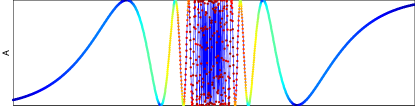
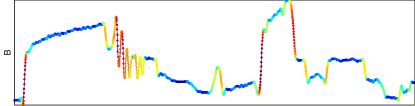
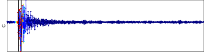
Figure 1: A, B, C: time series composed of $N^{\prime}=2072$ samples. The color of the signals A and B encodes the local variance (large = red, low = blue). C: seismogram; the color indicates the temporal proximity to a seismic arrival, identified by vertical black lines. See text for more details.

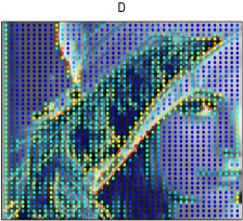
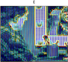
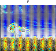
Figure 2: D, E, and F: image of size $128\times 128$, $128\times 128$, and $240\times 240$ pixels respectively. The color of the pixel at the center of each patch encodes the local variance of the image intensity.

Indeed, the distance defined by $\rho$ becomes useless when we need to compare very different patches (e.g. a patch of a uniform region vs a patch that contains an edge). As explained in section 4.2, the global organization of the patches can be discovered by studying the speed at which a random walk propagates along the graph (via hitting times).

Finally, we note that the weighted graph is fully characterized by its weight matrix.

Definition 2.4.

The weight matrix $\mathbf{W}$ is the $N\times N$ matrix with entries $\mathbf{W}_{n,m}=w_{n,m}$. The degree matrix is the $N\times N$ diagonal matrix $\mathbf{D}$ with entries $\mathbf{D}_{n,n}=\sum_{l=1}^{N}w_{n,l}$.

3 Warm up: A first look at the patch-set

The goal of this section is to provide the reader with some intuition about the geometry of the patch-set and the associated patch-graph. This will help us motivate our graph models and the analysis of their geometry. At the end of the section, we provide a sketch of our plan of attack.

3.1 Examples of signals and images

We construct the patch-set associated with some examples of signals and images. Because it is not practical to visualize the patch-set in $\mathbb{R}^{d}$ when $d=25$, we display the projection of the patch-set onto the three-dimensional space that captures the largest variance in the patch-set (computed using principal component analysis). Figure 1 displays three signals $\{x_{n}\},n=1,\ldots,N^{\prime}$, with $N^{\prime}=2072$. Patches of size $d=25$ samples are extracted around each time sample, which results in the maximum overlap between patches. Signal A is a chirp, signal B is a row of the image Lenna (shown in Fig. 2-D), and signal C is a seismogram [41].

In order to quantify the local regularity of signals A and B, we compute the variance over each patch, and color the curve according to the magnitude of the local variance: hot (red) for large variance and cold (blue) for low variance. The color of signal C encodes the temporal proximity to the arrival of a seismic wave associated with an earthquake: hot color indicates close proximity, while cold corresponds to baseline activity. Identifying arrival-times is necessary for purposes such as locating an earthquake’s epicenter. This example illustrates the application of the present work to the problem of detecting seismic waves [41].

Figure 2 displays three images. We extract patches of size $5\times 5$. Here, the patches are not maximally overlapping: we collect every third patch in the horizontal and vertical directions for images D and E, while we collect every fifth patch in each direction for image F. This results in patch-sets of size $42\times 42$ for images D and E, and of size $48\times 48$ for image F. As before, the color of a pixel in the images encodes the local variance within the patch centered at that pixel.

3.2 Projections of the patch-sets

Figure 3 shows the projections of each of the six patch-sets. Distances in Figure 3 correspond to the normalized distance $\rho$. We observe that patches with high variance (red-orange) appear to be scattered all over $\mathbb{R}^{d}$. These patches correspond to regions where the image intensity varies rapidly. Patches with low variance (blue-green), which correspond to regions where the signal is smooth and varies very little, tend to be concentrated along one-dimensional curves (for time series) and two-dimensional surfaces (for images). These visual observations can be confirmed when computing the actual mutual distances between patches (data not shown).

The organization of the patches in the patch-set can be explained using simple arguments. Let us assume that the sequence $\{x_{n}\}$ corresponds to the sampling of an underlying differentiable function $x(t)$, and assume that $x^{\prime}(t)$, the derivative of $x(t)$, remains small over the interval of interest. In this case, if two patches $\mathbf{x}_{n}$ and $\mathbf{x}_{m}$ overlap significantly – i.e. $|n-m|$ is small – then they will be close to one another in $\mathbb{R}^{d}$. Indeed, the values of the coordinates of patches $\mathbf{x}_{n}$ and $\mathbf{x}_{m}$ will be very similar, since the signal $x(t)$ varies slowly. In principle, if the sampling is fast enough, the patches should lie along a one-dimensional curve in $\mathbb{R}^{d}$. By the same argument, when $x(t)$ exhibits rapid changes, the magnitude of the derivative, $|x^{\prime}(t)|$, can be very large, and therefore temporally neighboring patches are not guaranteed to be spatial neighbors in $\mathbb{R}^{d}$. This argument allows us to understand the distribution of the patches in the signal B, or the image F.

Instead of characterizing patches according to the local smoothness of the underlying function, we can also analyze the distribution of the patches according to the function’s local frequency information. This will help us understand the structure of the patch-set for signal A.

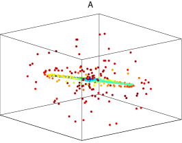
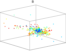
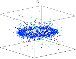
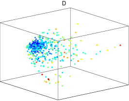
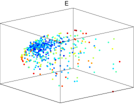
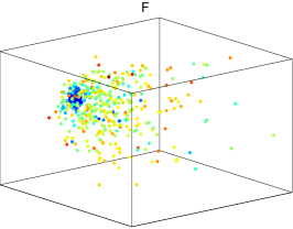
Figure 3: Principal component analysis of patch-sets associated with the time series A-C and the images D-F. Each point represents a patch; the color encodes the variance within the patch (see Figures 1 and 2.)

For this type of signal, it is appropriate to measure the distance between the normalized patches, $\mathbf{x}_{n}/\|\mathbf{x}_{n}\|$ and $\mathbf{x}_{m}/\|\mathbf{x}_{m}\|$ after computing the Fourier transforms (a simple rotation of $\mathbb{R}^{d}$) of the respective patches. This process is akin to the concept of time-frequency analysis. We expect that regions of the signal with little local frequency changes will cluster in $\mathbb{R}^{d}$: this is the case for the blue patches of the chirp A. On the contrary, when the local frequency content changes rapidly (as in the middle of the chirp A), the corresponding (red/orange) patches will be at a large distance of one another in $\mathbb{R}^{d}$ (see Figure 3-A).

Finally, we can try to understand the organization of the patch-set for the seismogram C. Let us assume that $\{x_{n}\}$ is obtained by sampling a function of the form $x(t)=b(t)+w(t)$, where $w(t)$ represents a seismic wave and $b(t)$ represents baseline activity. We can expect that $w(t)$ is a rapidly oscillating transient with a rich frequency content, while $b(t)$ is varying slowly. Now consider two patches $\mathbf{x}_{n}$ and $\mathbf{x}_{m}$. It can be shown that if both patches $\mathbf{x}_{n}$ and $\mathbf{x}_{m}$ are extracted from the baseline function, $b(t)$, and do not contain any part of the energetic transient, then their mutual distance is expected to be small. In addition, if $\mathbf{x}_{n}$ contains part of the energetic transient $w(t)$ and $\mathbf{x}_{m}$ is extracted from the baseline $b(t)$, then their mutual distance is expected to be large. Finally, if $\mathbf{x}_{n}$ and $\mathbf{x}_{m}$ are composed of two different parts of $w(t)$, then their mutual distance is also expected to be large (provided the patches are sufficiently long and $w(t)$ oscillates sufficiently fast). More generally, one can expect that two patches extracted from two different energetic transients $w_{1}(t)$ and $w_{2}(t)$ will be at a large distance from one another [41].

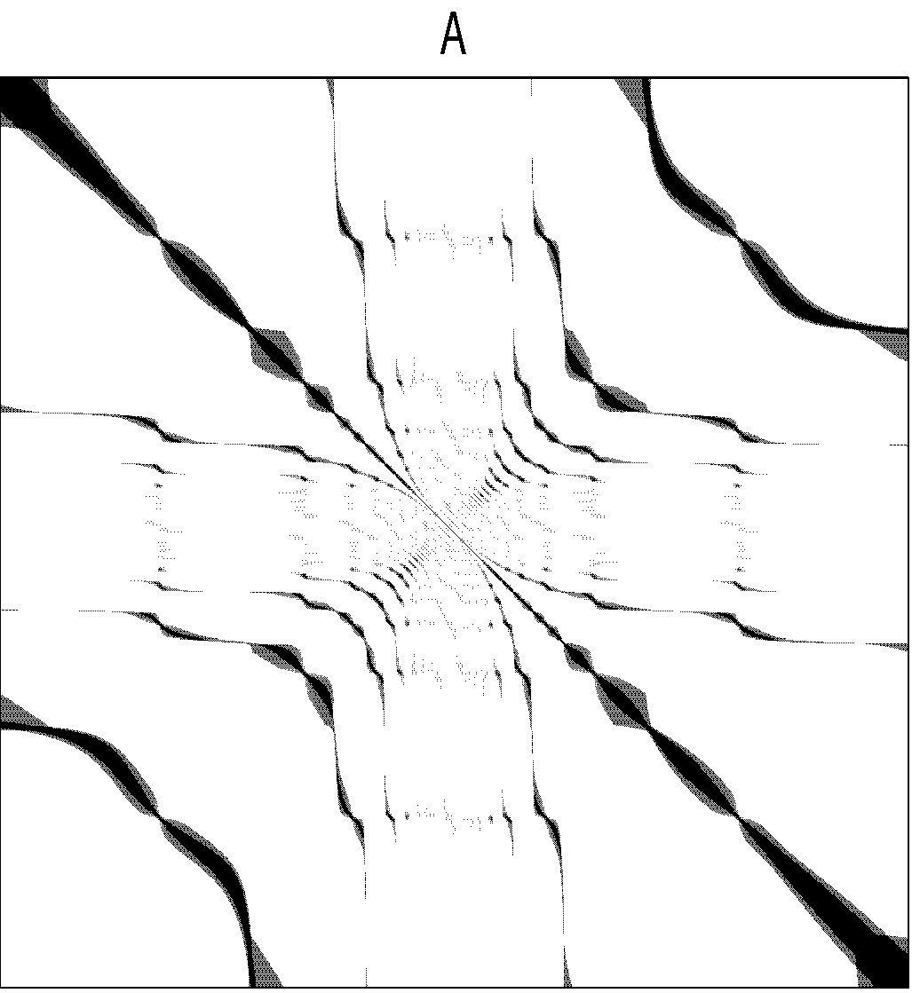
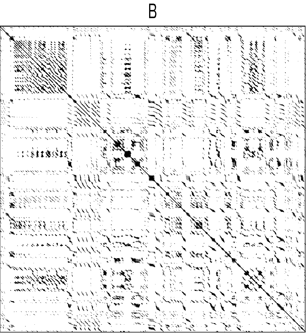
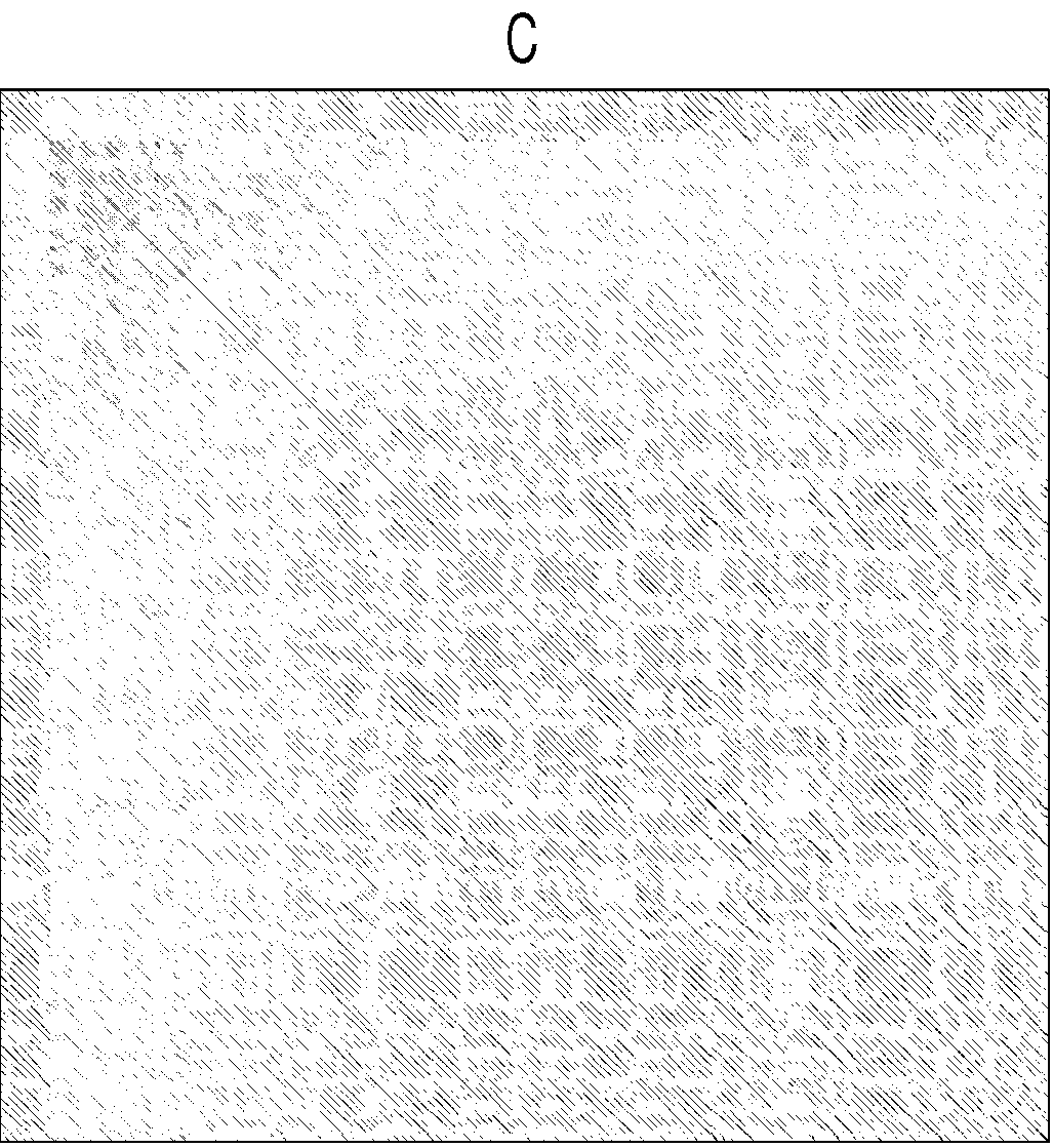
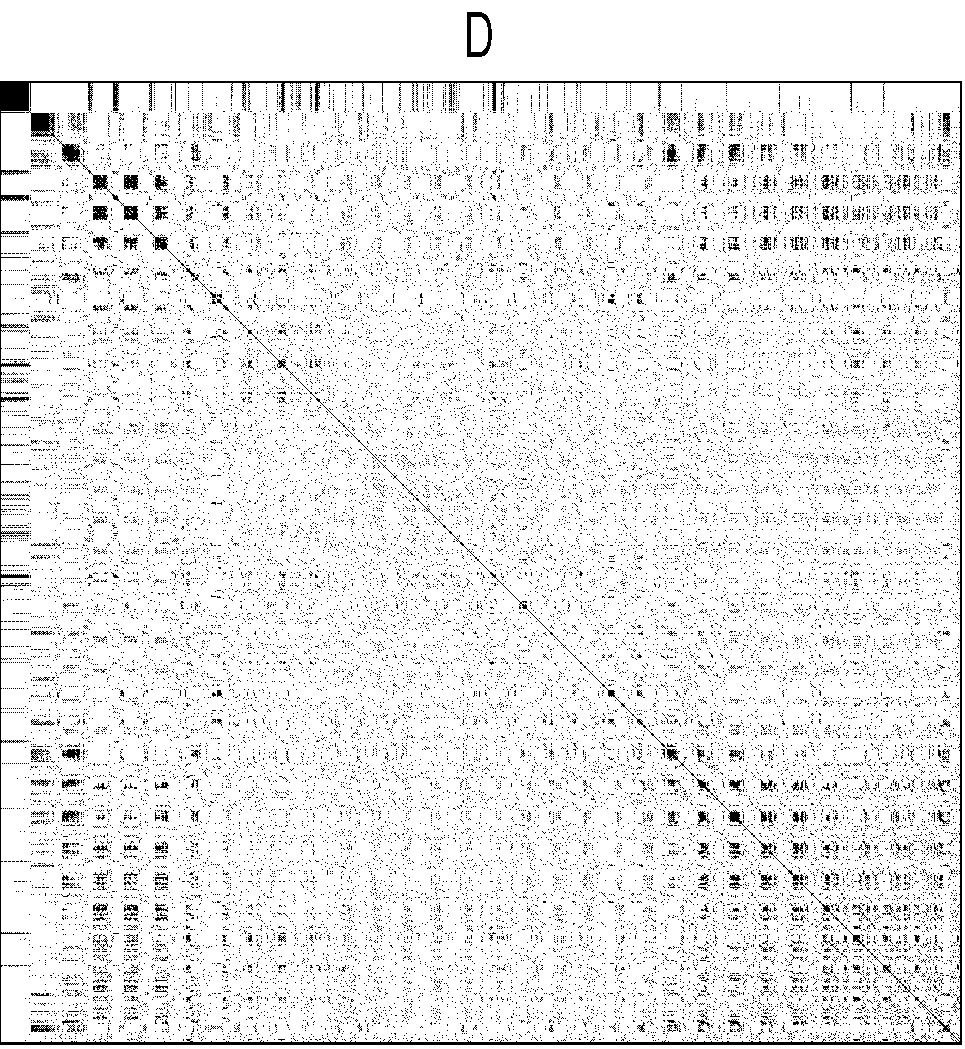
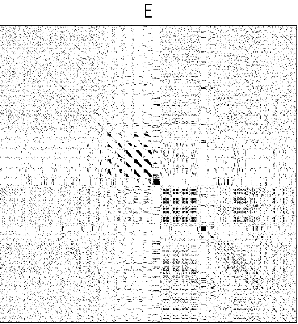
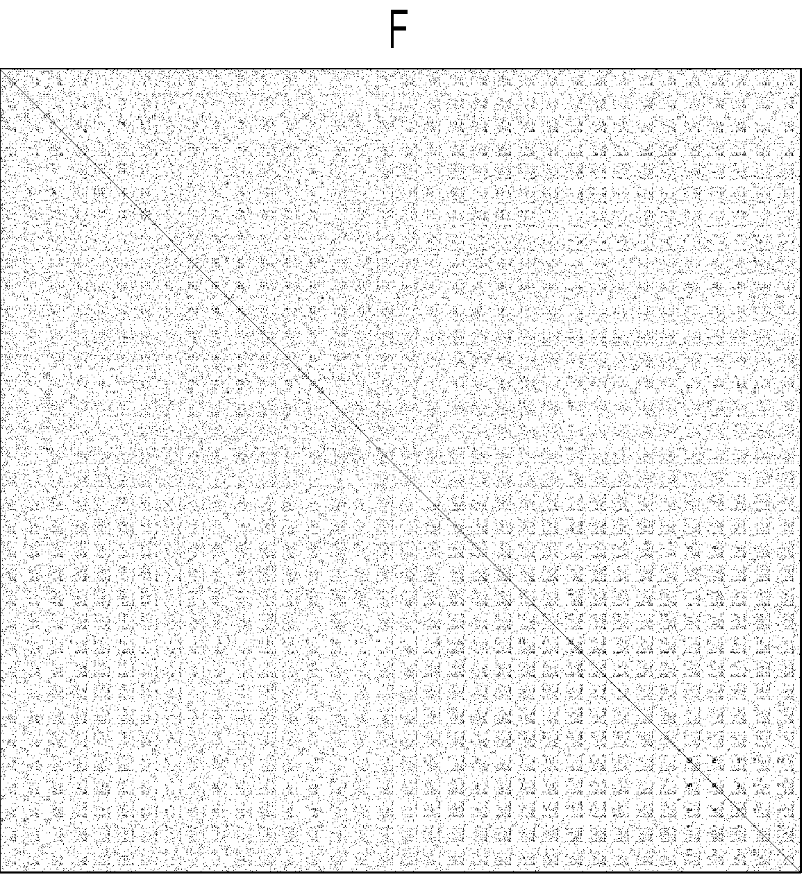
Figure 4: The weight matrices $\mathbf{W}$ associated with signals A-F are displayed as images: $w_{n,m}$ is encoded as a grayscale value: from white ($w_{n,m}=0$) to black $(w_{n,m}=1)$. Dark structures along the diagonal of the $\mathbf{W}$ matrix associated with the time series A-C indicate that patches that are close in time are also close in $\mathbb{R}^{d}$.

3.3 From the patch-set to the patch-graph: the weight matrix $\mathbf{W}$

Having gained some understanding about the organization of the patch-set, we now move to the structure of the patch-graph and its weight matrix $\mathbf{W}$. Figure 4 displays the weight matrices built from the patch-sets that correspond to the time series A-C (top) and the images D-F (bottom). Note that when processing time series A-C, the columns (or equivalently, the rows) of $\mathbf{W}$ can be identified with temporally-ordered time-samples. Therefore, a large main diagonal in the weight matrix correspond to patches that are close in time and also close in $\mathbb{R}^{d}$. For instance, consider the time series A and its associated weight matrix. The dark bands near the top-left and bottom-right of the diagonal correspond to the slowly-varying oscillations near the beginning and end of the chirp (see Figure 1). Indeed, large entries in the diagonal of $\mathbf{W}$ is a direct consequence of relatively little variation in the time series. On the other hand, the columns of $\mathbf{W}$ corresponding to portions of the time series that exhibit rapid local changes (center of Figure 4-A) tend to lack such prominent diagonal structures. For such regions of the matrix $\mathbf{W}$, the entries are no longer concentrated along the diagonal, and are shattered across all rows and columns (see the center of $\mathbf{W}$ in Figure 4-A; the columns correspond to the fastest oscillations at the center of the chirp). The large distances between these patches are also apparent in the lighter pixel intensities, representing relatively smaller edge-weights. Note that the patches extracted from the seismic data are very far apart, as indicated by the much lighter shades of gray. It is more difficult to relate the ordering of an image’s weight matrix to locations in the image itself. For the weight matrices associated with images D-F, the ordering of the columns is equivalent to the order in which the patches were collected from the image plane: first left-to-right, then top-to-bottom (similar to a raster scan, or how one would read pages of a book). Hence, periodically repeating dark blocks in the weight matrices associated with images D-F are indicative of image patches that are close in $\mathbb{R}^{d}$ and close in the image-plane as a result of relatively little change in the image’s local content. For example, the dark square-like structure that appears near the main diagonal of $\mathbf{W}$ in Figure 4-E, and which spans roughly one fifth of the number of columns, corresponds to the mirror’s smooth, light border in image E.

3.4 Summary of the experiments and our plan of attack

The experiments in sections 3.1 and 3.3 highlight the fact that regions of an image, or of a signal, that contain anomalies (e.g. singularities, edges, rapid changes in the frequency content, etc.) are scattered all over the patch-set, making their detection and identification extremely difficult (see Figures 3-A and 3-F). In contrast, patches from smooth regions appear to cluster along low dimensional curves or surfaces. Because the anomalous patches are usually the most interesting ones, we need to find a new parametrization of the patch-set that concentrates the anomalies and separate them from the smooth baseline part of the image. The structure of $\mathbf{W}$ in the “rough regions” suggest that patches that contain anomalies appear to be very well connected (see the center of Figure 4-D, which corresponds to the boa on the hat of Lenna). This concept can be quantified by studying how fast a random walk would reach all patches in these rough regions of $\mathbf{W}$, and suggest that we should consider studying the hitting times associated with a random walk on the patch-graph. In the next section we formalize this concept and propose a parametrization of the patch-set in terms of commute time. A theoretical analysis of this approach is provided in section 5

4 Parametrizing the patch-graph

4.1 The fast and slow patches

We first introduce the concept of fast and slow patches. We have noticed that patches that contain anomalies (discontinuities, edges, fast changes in frequency, etc.) in the original signal lead to regions of the matrix $\mathbf{W}$ where the nonzero entries are scattered all around. We call such patches fast patches because, as we will see in the following, a random walk will diffuse extremely fast in such regions of the patch-graph. Conversely smooth regions of the signal lead to slow patches that are associated with a small number of large entries in $\mathbf{W}$, which are concentrated along the diagonal. A random walk initialized in the slow patch region of the patch-graph will diffuse very slowly.

4.2 A better metric on the graph: the commute time

As explained previously, we propose to replace the Euclidean distance, which leads to the scattering of the fast patches seen in Figure 3 by a notion of distance that quantifies the speed at which a random walk diffuses on the patch-graph. We propose to use the commute time. Parametrizing the graph using its commute time distance is closely related to parametrizing the graph using its diffusion distance [14, 23] (see Section 4.2.2). Although the works [7, 37, 38] do not explicitly embed vertices of the patch-graph based on the diffusion distance, they also study a random walk on the patch-graph, and define the diffusion distance in terms of this walk. In these studies, noise is removed by evolving the diffusion process for a small time. A detailed comparison of our approach with the seminal work of [37] is provided in section 7.3. We note that the notion of first-passage time associated with a diffusion (which is equivalent to the hitting time associated with a random walk) has been used extensively to characterize the geometry of complex networks, and random media (e.g. [3, 15] and references therein). It is therefore natural to analyze the patch-set with this distance.

4.2.1 A random walk on the patch-graph

In order to define the commute time between two vertices, we first need to define a random walk on the graph. In our problem, the random walk does not correspond to a physical process, but will lead to a notion of global proximity between patches. We consider a first-order homogeneous Markov process, $Z_{k}$, defined on the vertices of the patch-graph, $\Gamma$, and evolving with the transition probability matrix $\mathbf{P}$ given by

$$\mathbf{P}_{n,m}=$$ (5)

Consider a slow patch $\mathbf{x}_{n}$ extracted from a regular/smooth part of the signal. If the random walk starts at $\mathbf{x}_{n}$, then it can only travel along the low-dimensional structure that corresponds to the temporal neighbors of $\mathbf{x}_{n}$ (see e.g. Figure 3-A.) The existence of this narrow bottleneck is also visible in the $\mathbf{W}$ matrix (see Figure 4-A): a random walk initialized within the fat diagonal of the upper left corner of $\mathbf{W}$ (the low frequency part of the chirp) is trapped in this region of the matrix, and can only travel along this fat diagonal. As a result, it will take many steps for the random walk to reach another slow patch $\mathbf{x}_{m}$ if $|n-m|$ is large. This notion can be quantified by computing the average hitting-time, $h(\mathbf{x}_{n},\mathbf{x}_{m})$, which measures the expected minimum number of steps that it takes for the random walk, started at vertex $\mathbf{x}_{n}$, to reach the vertex $\mathbf{x}_{m}$ [6]

$$h(\mathbf{x}_{n},\mathbf{x}_{m})={}_{n}\min\{j\geq 0:Z_{j}=\mathbf{x}_{m}\},$$

where the expectation _n is computed when the random walk is initialized at vertex $\mathbf{x}_{n}$, i.e. when $Z_{0}=\mathbf{x}_{n}$. The commute time [6]: provides a symmetric version of $h$, and is defined by

$$\kappa(\mathbf{x}_{n},\mathbf{x}_{m})=h(\mathbf{x}_{n},\mathbf{x}_{m})+h(\mathbf{x}_{m},\mathbf{x}_{n}).$$ (6)

4.2.2 Spectral representation of the commute time

When the random walk is reversible and the graph is fully connected, the commute time can be expressed using the eigenvectors $\phi_{1},\ldots,\phi_{N}$ of the symmetric matrix

$$\mathbf{D}^{-1/2}\mathbf{W}\mathbf{D}^{-1/2}=\mathbf{D}^{1/2}\mathbf{P}\mathbf{D}^{-1/2}.$$

The corresponding eigenvalues can be labeled such that $-1<\lambda_{N}\leq\ldots\leq\lambda_{2}<\lambda_{1}=1$. Each eigenvector $\phi_{k}$ is a vector with $N$ components, one for each vertex of the graph. Hence, we write

$$\phi_{k}=\begin{bmatrix}\phi_{k}(\mathbf{x}_{1})&\phi_{k}(\mathbf{x}_{2})&\ldots&\phi_{k}(\mathbf{x}_{N})\end{bmatrix}^{T},$$

to emphasize the fact that we consider $\phi_{k}$ to be a function sampled on the vertices of $\Gamma$. The commute time can be expressed as

$$\kappa(\mathbf{x}_{n},\mathbf{x}_{m})=\sum_{k=2}^{N}\frac{1}{1-\lambda_{k}}\left(\frac{\phi_{k}(\mathbf{x}_{n})}{\sqrt{\pi_{n}}}-\frac{\phi_{k}(\mathbf{x}_{m})}{\sqrt{\pi_{m}}}\right)^{2},$$ (7)

where $\pi_{n}=\sum_{m=1}^{N}w_{n,m}/\sum_{j,l=1}^{N}w_{j,l}$ is the stationary distribution associated with the transition probability matrix $\mathbf{P}$ [27, 36].

4.2.3 The relationship to diffusion maps

The diffusion distance [14] between vertices $\mathbf{x}_{m}$ and $\mathbf{x}_{n}$, $D_{t}(\mathbf{x}_{m},\mathbf{x}_{n})$, measures the distance between the transition probability distributions – computed at time $t$ – of two random walks initialized at $\mathbf{x}_{n}$ and $\mathbf{x}_{m}$, $\sum_{l=1}^{N}|\mathbf{P}^{(t)}_{n,l}-\mathbf{P}^{(t)}_{m,l}|^{2}$. The diffusion distance can also be decomposed in terms of the eigenvectors $\phi_{k}$ [14],

$$D^{2}_{t}(\mathbf{x}_{m},\mathbf{x}_{n})=\frac{1}{V}\sum_{k=2}^{N}\lambda_{k}^{2t}\left(\frac{\phi_{k}(\mathbf{x}_{m})}{\sqrt{\pi_{m}}}-\frac{\phi_{k}(\mathbf{x}_{n})}{\sqrt{\pi_{n}}}\right)^{2},$$ (8)

where $V=\sum_{m^{\prime},n^{\prime}}w_{m^{\prime},n^{\prime}}$ is the volume of the graph. It follows that the commute time is a scaled sum of the squares of diffusion distances computed at all times,

$$\kappa(\mathbf{x}_{m},\mathbf{x}_{n})=V\sum_{t=0}^{\infty}D^{2}_{t/2}(\mathbf{x}_{m},\mathbf{x}_{n}).$$ (9)

The significance of this equation is that the commute time includes the short term evolution ($t\approx 0$) as well as the asymptotic regime ($t\rightarrow\infty$) of the random walk. We will come back to this analysis in section 5.4.

4.3 Parametrizing the patch-graph

Equation (7) suggests the following embedding $\Psi$ of the patch-graph $\Gamma$ into $\mathbb{R}^{N-1}$,

$$\Psi:\mathbf{x}_{n}\longrightarrow\frac{1}{\sqrt{\pi_{n}}}\begin{bmatrix}\frac{\phi_{2}(\mathbf{x}_{n})}{\sqrt{1-\lambda_{2}}}&\frac{\phi_{3}(\mathbf{x}_{n})}{\sqrt{1-\lambda_{3}}}&\ldots&\frac{\phi_{N}(\mathbf{x}_{n})}{\sqrt{1-\lambda_{N}}}\end{bmatrix}^{T},\qquad n=1,2,\ldots,N.$$ (10)

If we agree to measure the distance on the graph $\Gamma$ using the square root of the commute time, then the mutual Euclidean distance after embedding is equal to the original distance on the graph,

$$\|\Psi(\mathbf{x}_{n})-\Psi(\mathbf{x}_{m})\|=\sqrt{\kappa(\mathbf{x}_{n},\mathbf{x}_{m})}.$$ (11)

The result is a direct consequence of (8) and (9). Similar ideas were first proposed in [32] to embed manifolds and are the foundation of the parametrizations given in [2, 14]. In practice, we need not use all the $N-1$ coordinates in the embedding defined by (10). Indeed, since $\lambda_{N}\leq\cdots\leq\lambda_{2}<\lambda_{1}$, we have that $\tfrac{1}{\sqrt{1-\lambda_{N}}}\leq\cdots\leq\tfrac{1}{\sqrt{1-\lambda_{3}}}\leq\tfrac{1}{\sqrt{1-\lambda_{2}}}$, and therefore, if we can accept some approximation error, we can use only the first $d^{\prime}$ coordinates of $\Psi$. As we will see in section 5.4, this dimension reduction further improves the separation between slow patches and fast patches. In the remaining of the paper we will work with the embedding of $\Gamma$ into $\mathbb{R}^{d^{\prime}}$ defined by

$$\Phi:\mathbf{x}_{n}\longrightarrow\frac{1}{\sqrt{\pi_{n}}}\begin{bmatrix}\frac{\phi_{2}(\mathbf{x}_{n})}{\sqrt{1-\lambda_{2}}}&\ldots&\frac{\phi_{d^{\prime}+1}(\mathbf{x}_{n})}{\sqrt{1-\lambda_{d^{\prime}+1}}}\end{bmatrix}^{T}.$$ (12)

We note that we can always choose $d^{\prime}$ such that the embedding $\Phi$ almost preserves the commute time,

$$\|\Phi(\mathbf{x}_{n})-\Phi(\mathbf{x}_{m})\|^{2}\approx\kappa(\mathbf{x}_{n},\mathbf{x}_{m}).$$ (13)

In fact, our experiments indicate that this approximation holds for small values of $d^{\prime}$.

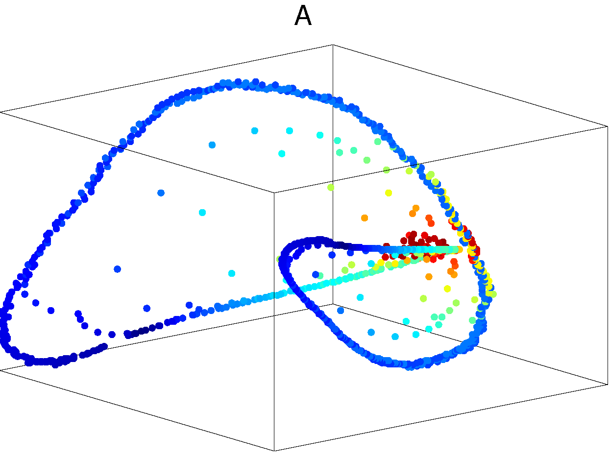
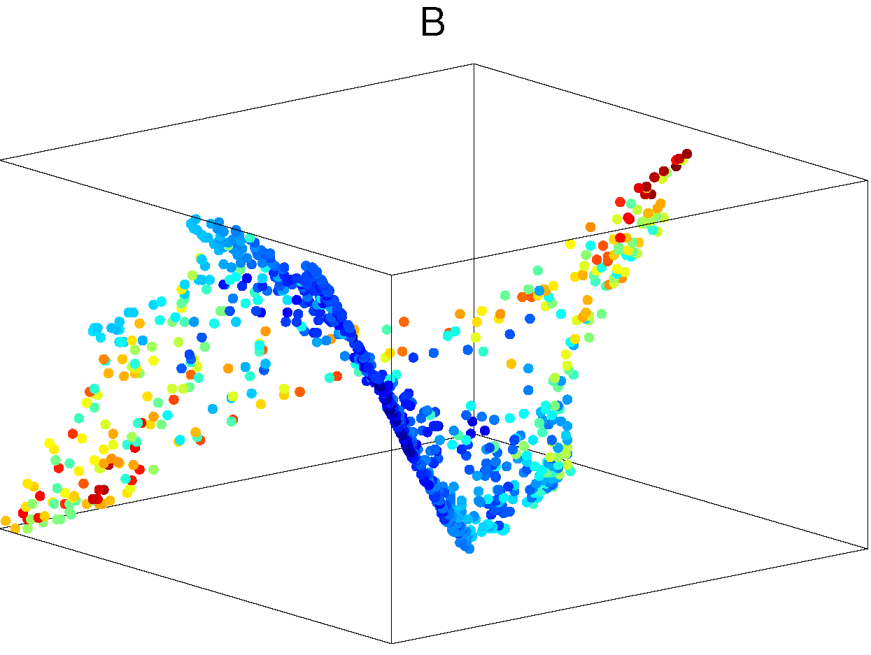
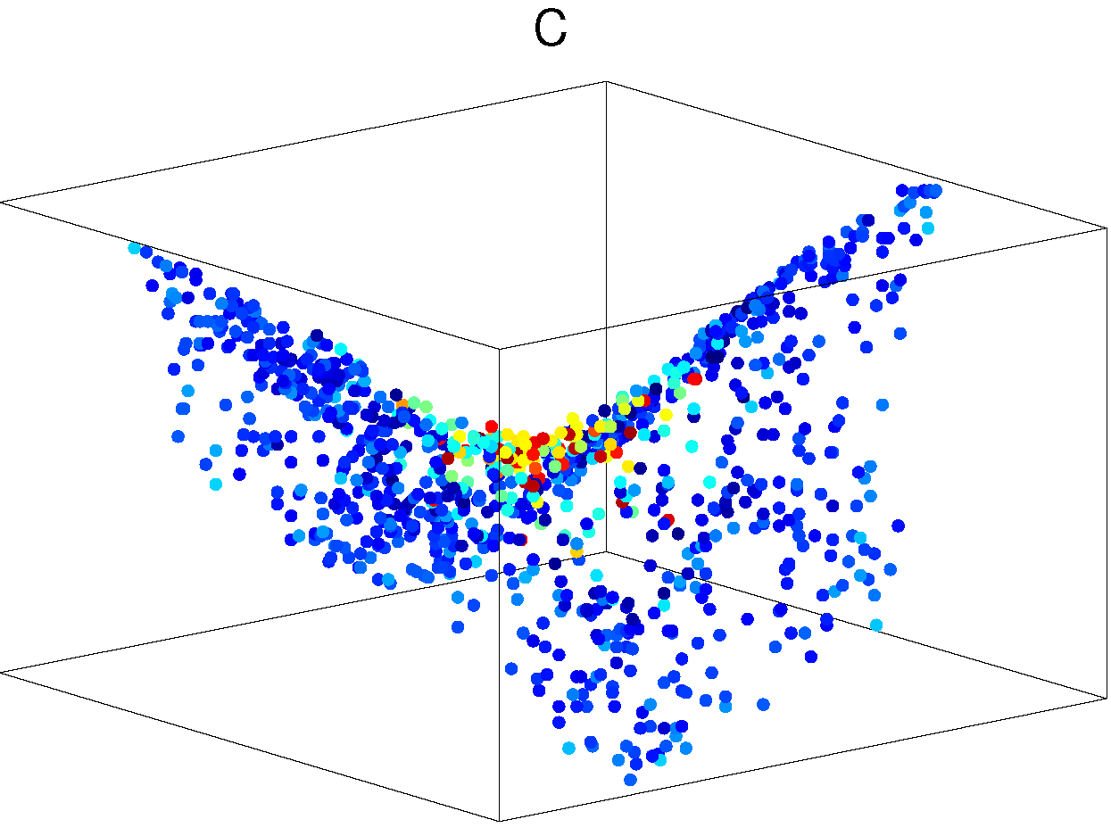
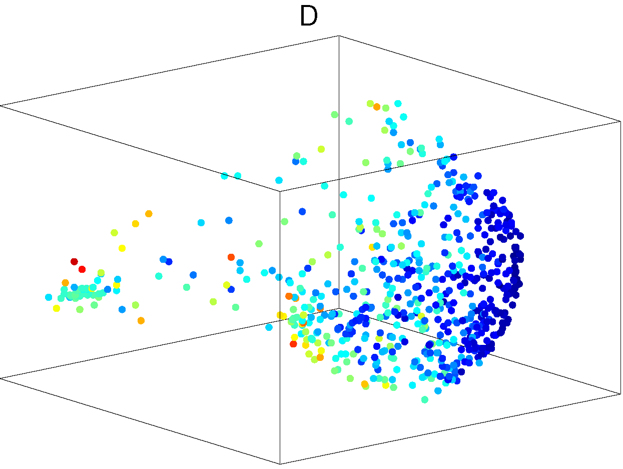
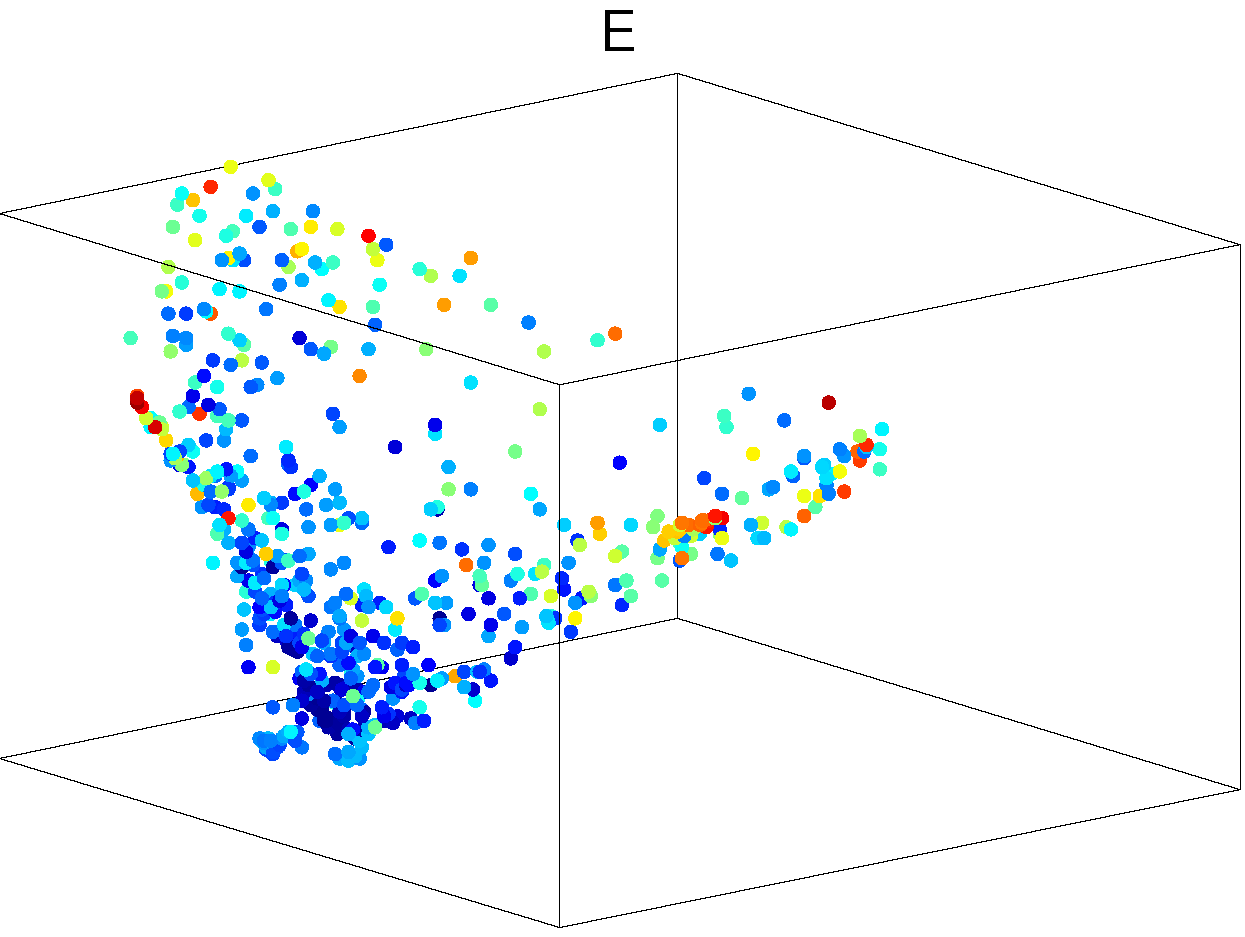
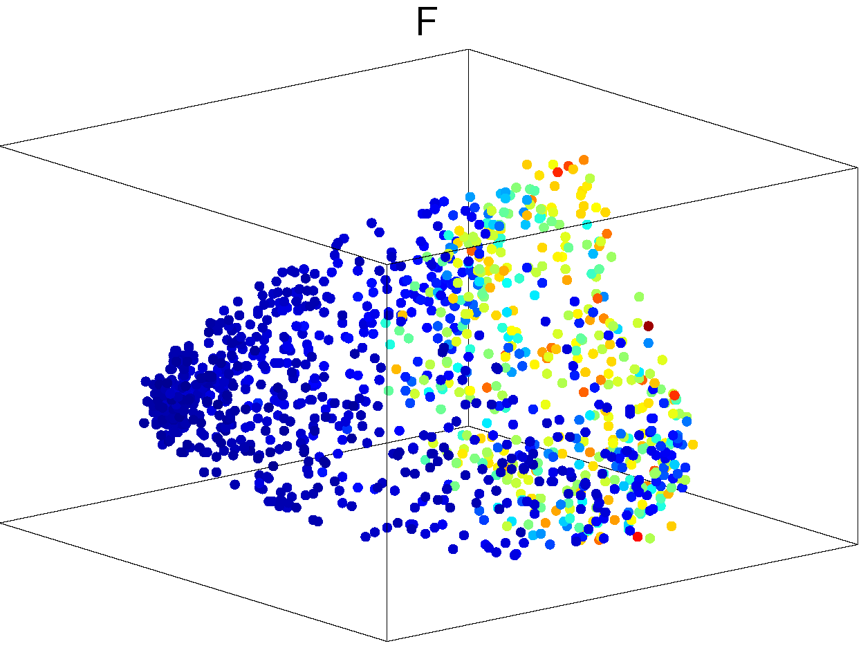
Figure 5: Scatter plot of the patch-set shown in Figure 3 after parametrizing using $\Phi$ in (12), with $d^{\prime}=3$. The fast patches (red and orange) are now concentrated and have been lumped together. The slow patches (blue-green) remain aligned along curves (for time-series) and surfaces (for images).

4.4 Examples (revisited)

Figure 5 displays the embedding of the patch-sets associated with signals and images A-F using the map $\Phi$ (12), where $d^{\prime}=3$. The blue curve in Figure 5-A corresponds to the slow patches (low frequencies of the chirp) that are connected according to their temporal proximity. On the other hand, red and orange patches extracted from the high frequency part of the chirp are now concentrated in a relatively small region (compare to Figure 3-A). Similar features are seen in the parametrizations of the patch-graphs associated with signals B-F.

5 A model for the patch-graph and the analysis of its embedding

5.1 Our approach

The embedding of the patch-graph $\Gamma$ defined by $\Phi$, in (12), should lead to a representation of the patch-set in $\mathbb{R}^{d^{\prime}}$ where distances correspond to commute times measured along the graph before embedding. Our goal is to explain the concentration of the fast patches created by the embedding $\Phi$ (see e.g. Figure 5). Our approach is based on a theoretical analysis of a graph model that epitomizes the characteristic features observed in patch-graphs composed of a mixture of fast and slow patches. This model is composed of two subgraphs: a subgraph of slow patches, which are extracted from the smooth regions of the signal, and a subgraph of fast patches, which are extracted from the regions of the signal that contain singularities, changes in frequency, or energetic transients. We confirm our theoretical analysis with numerical experimentations using synthetic signals in section 6, and we demonstrate that our conclusions are in fact applicable to a larger class of patch-graphs. The graph models are introduced in section 5.2. Our theoretical analysis of the embedding of the graph models is given in section 5.3. We evaluate the performance of the embedding $\Phi$ when $d^{\prime}$ is small in section 5.4.

5.2 The prototypical graph models

We define the graph models in terms of the nonzero entries in the associated weight matrix $\mathbf{W}$. Without loss of generality, we assume that the number of vertices $N$ is even.

The slow graph model

The large entries in a weight matrix $\mathbf{W}$ of a patch-graph composed only of slow patches will have large entries when $|n-m|$ is small: temporal/spatial proximity implies proximity in patch-space (see e.g. Figure 4-A, top corner). We therefore define the slow graph model as follows.

Definition 5.1.

The slow graph $\mathcal{S}(N,L)$ is a weighted graph composed of $N$ vertices,

$\mathbf{x}_{1},\ldots,\mathbf{x}_{N}$. The weight on the edge $\{\mathbf{x}_{n},\mathbf{x}_{m}\}$ is defined by

$$w_{n,m}=\begin{cases}w_{\mathcal{S}}&\text{if $|n-m|\leq L$},\\ 0&\text{otherwise,}\end{cases}\qquad\text{for}\quad 1\leq n,m\leq N\quad\text{and}\quad 2L+1\leq N.$$ (14)

The weight $w_{s}$ is a positive real number that models the distance between two temporally adjacent patches. The parameter $L$ characterizes the thickness of the diagonal in $\mathbf{W}$. The slow graph is fully connected and each vertex has at most $2L$ neighbors, not including self-connections (see Figure 6). Hence, we require that $2L+1\leq N$. Finally, note that the slow graph is distinct from a regular ring, since the first and last vertices are not connected. We do not consider a regular ring since it would imply that the underlying signal is periodic.

The fast graph model

We now consider the model for a patch-graph built from a patch-set comprising only fast patches. As demonstrated in section 3, most of the entries in $\mathbf{W}$ have similar sizes, and appear to be scattered throughout the matrix: temporal/spatial proximity does not correlate with proximity in patch space. In fact, fast patches are all far away from one another. We therefore define the fast graph model as follows.

Definition 5.2.

The fast graph $\mathcal{F}(N,p)$ is a random weighted graph composed of $N$ vertices, $\mathbf{x}_{1},\ldots,\mathbf{x}_{N}$. The weight on the edge $\{\mathbf{x}_{n},\mathbf{x}_{m}\}$ is defined by

$$w_{n,m} = w_{m,n}=\begin{cases}w_{\mathcal{F}}&\text{with probability $p$},\\ 0&\text{with probability $1-p$}\end{cases}\quad\text{if $1\leq n<m\leq N$},$$

and

$$w_{n,m} = 1\quad\text{if}\quad n=m.$$

The weight $w_{F}$ is a positive real number that models the distance between two fast patches. The fast graph model is equivalent to a weighted version of the Erdös-Renyi graph model [19], except that $\mathcal{F}(N,p)$ contains self-connections and has edge weights possibly less than one. The parameter $p$ controls the density of the edges; $p=1$ corresponds to a fully connected graph (clique).

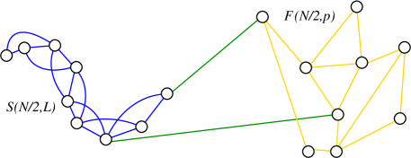
Figure 6: The fused graph model $\Gamma^{\ast}(N)$ is composed of a slow graph $\mathcal{S}(N/2,L)$ (blue) and a fast graph $\mathcal{F}(N/2,p)$ (orange), connected by random edges (green).

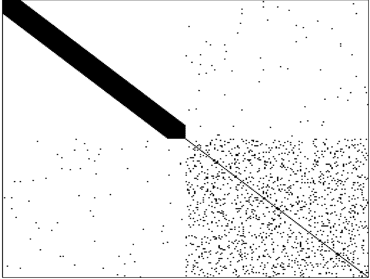
Figure 7: The weight matrix $\mathbf{W}$ of the fused graph model $\Gamma^{\ast}(256)$ is displayed as an image: $w_{n,m}$ is encoded as a grayscale value: from white ($w_{n,m}=0$) to black $(w_{n,m}=1)$. The entries of $\mathbf{W}$ associated with the slow graph appear in the upper-left quadrant of $\mathbf{W}$. Entries associated with the fast graph appear in the lower right quadrant. Random edges between the fast graph and slow graph appear in the upper right and lower left quadrants.

The fused graph model

The fused graph model exemplifies the patch-set associated with a signal, or an image, which exhibits regions of fast and slow changes. The fused graph combines a slow and a fast subgraph of equal size (see Figure 6).

Definition 5.3.

The fused graph $\Gamma^{\ast}(N)$ is a weighted graph composed of a slow subgraph $\mathcal{S}(N/2,L)$ and a fast subgraph $\mathcal{F}(N/2,p)$. In addition, edges between $\mathcal{S}(N/2,L)$ and $\mathcal{F}(N/2,p)$ are created randomly and independently with probability $q$ and assigned the edge weight $w_{c}>0$.

Edges between $\mathcal{S}(N/2,L)$ and $\mathcal{F}(N/2,p)$ ensure that $\Gamma^{\ast}(N)$ is connected (a requirement for the validity of the parametrization (10)). These edges allow us to model patches that are extracted from regions of the image that combine edges/transients and smooth intensity. If $q$ is so small that no edges are created between the two subgraphs, then an edge is placed at random between the two subgraphs to ensure that the final fused graph is connected.

The true patch-graph is always constructed using a $\nu$ nearest neighbor rule (see section 2): each patch is connected to $\nu$ other patches. In order to mimic a true patch-graph, we adjust the thickness $L$ of the slow subgraph to the density of the edge connection, $p$, in the fast subgraph, so that on average, each vertex in the fused graph is connected to $2L$ vertices. We know that the number of edges between distinct vertices in $\mathcal{F}(N,p)$ is a binomial random variable with expectation $\tfrac{N(N-1)}{2}p$. Since the total number of edges between distinct vertices of $\mathcal{S}(N,L)$ is equal to

$$\sum_{j=1}^{L}(N-j)=NL-\frac{L(L+1)}{2},$$ (15)

we choose

$$p=\frac{2L}{N-1}-\frac{L(L+1)}{N(N-1)}.$$ (16)

This choice of $p$ guarantees that the expected number of edges in $\mathcal{F}(N,p)$ is equal to the number of edges in $\mathcal{S}(N,L)$. Furthermore, provided that $L=\mathcal{O}(\ln(N))$, a short computation shows that, for large values of $N$, this choice of $p$ also ensures that the expected degree of a vertex in $\mathcal{F}(N,p)$ is equal to the average degree of a vertex in $\mathcal{S}(N,L)$. Figure 7 shows the nonzero entries in the weight matrix associated with one realization of the fused graph model using parameters $N=256$, $L=\left\lceil 2\ln N\right\rceil=12$ and $q=\tfrac{1}{N}$. Vertices $\mathbf{x}_{n}$ with $n\leq 128$ are only connected to other vertices $\mathbf{x}_{m}$ if $|n-m|\leq L$. This connectivity mimics the spatial (temporal) connectivity present in the smooth parts of an image (signal).

5.3 The main result

Our goal is to understand the effect of the embedding $\Phi$ defined by (12) on the fused graph. It turns out that studying the embedding of each individual subgraph (slow and fast) separately is much more tractable than considering the entire fused graph. To complement our theoretical study of the fast and the slow subgraphs, we provide numerical evidence in sections 5.4 that indicates that our understanding of the embedding of the subgraphs can be used to analyze the embedding of the fused graph. In section 6, we confirm that our theoretical analysis can be applied to true patch-graphs. Instead of studying $\Phi$ directly, we take advantage of the fact that the embedding $\Phi$ almost preserves the commute time (see (13)). We can therefore understand the effect of the embedding on the distribution of mutual distances $\|\Phi(\mathbf{x}_{n})-\Phi(\mathbf{x}_{m})\|$ within a subgraph by studying the distribution of the commute times $\kappa(\mathbf{x}_{n},\mathbf{x}_{m})$ on that subgraph. While it would appear that it is a straightforward affair to compute the commute time on the slow graph, the computation becomes rapidly intractable. For this reason we provide lower and upper bounds for the average commute time on the slow and fast subgraphs, respectively. This is sufficient for our needs, since the two bounds rapidly separate even for low values of $N$. To estimate these bounds, we rely on the connection between commute times on a graph and effective resistance on the corresponding electrical network [10, 16]. Specifically, we map a graph to an electrical circuit as follows: each edge with weight $w_{n,m}$ becomes a resistor with resistance $1/w_{n,m}$. The vertices of the graph are the connections in the circuit. Given two vertices, $\mathbf{x}_{n}$ and $\mathbf{x}_{m}$ in the circuit, one can compute the effective resistance between these nodes, $R_{n,m}$. The key result [10] is that $\kappa(\mathbf{x}_{n},\mathbf{x}_{m})=VR_{n,m}$, where $V$ is the volume of the graph.

Before stating the main Lemma, let us take a moment to compute some rough estimates of the commute times on the slow and fast graphs. To get some quick answers, we consider the simplest versions of the two graph models. When $L=1$, the slow graph $\mathcal{S}(N,1)$ is a path with self-connections. On a path of $N$ vertices without self-connections, the commute time between vertex $\mathbf{x}_{n}$ and $\mathbf{x}_{m}$ is equal to $2(N-1)|m-n|$. Therefore, the average commute time (computed over all pairs of vertices) on a path of length $N$ is $\mathcal{O}(N^{2})$. While it would make sense that adding edges to a path should decrease the commute time, this is usually not true [27]. Nevertheless, the presence of edges that allow the random walk to move forward by a distance $L$ at each time step lead us to conjecture that the average commute time on $\mathcal{S}(N,L)$ should be of the order $\frac{1}{L}\mathcal{O}(N^{2})$. In fact, as we will see in Lemma 5.6, the average commute time of the slow graph is of the order $\frac{1}{L^{2}}\mathcal{O}(N^{2})$. With regard to the fast graph, we can analyze the case where the density of edges $p=1$. In this case, the fast graph $\mathcal{F}(N,1)$ is a complete graph, or clique, and every vertex is connected to every other vertex. In a complete graph, the average commute time is $\mathcal{O}(N)$. Since the fast graph can be regarded as a complete graph whose edges have been removed with probability $1-p$, we expect the commute time to be slightly larger than $\mathcal{O}(N)$, since removing edges restricts the random walker’s options to get from one vertex to another. Again, in agreement with our intuition, Lemma 5.6 asserts that in the fast graph, the commute time is of the order of $[L\ln(N)/\ln(L)]\mathcal{O}(N)$.

We are now ready to state the main lemma. Our results will be stated in terms of the “average behavior” of the commute time on each graph, a concept that we need to define properly. In the case of the slow graph, which is deterministic, we consider the average commute time computed over all pairs of vertices.

Definition 5.4.

Let $\kappa_{\mathcal{S}}$ be the average commute time between vertices in the slow graph $\mathcal{S}(N,L)$

$$\kappa_{\mathcal{S}}\triangleq\frac{2}{N(N-1)}\sum_{1\leq m<n\leq N}\kappa(\mathbf{x}_{n},\mathbf{x}_{m}).$$ (17)

In the case of the fast graph, the “average behavior” of the commute time needs to be defined more carefully. Indeed, each fast graph is a realization of a stochastic process, and therefore we need to consider the expectation of the commute time. More precisely, given a realization, $\mathcal{F}$, of a fast graph, we compute the expected commute time ${}_{\mathbf{x}_{n},\mathbf{x}_{m}}\left[\kappa|{\mathcal{F}}\right]$ as the expectation of $\kappa(\mathbf{x}_{m},\mathbf{x}_{n})$ over all possible random assignment of the vertices $\mathbf{x}_{n}$ and $\mathbf{x}_{m}$. We then need to consider how ${}_{\mathbf{x}_{n},\mathbf{x}_{m}}\left[\kappa|{\mathcal{F}}\right]$ varies as a function of $\cal F$. Therefore, we compute a second expectation over all possible random graphs $\mathcal{F}$.

Definition 5.5.

The expected commute time $\kappa_{\mathcal{F}}$ on a fast graph $\mathcal{F}$ generated according to (5.2) is defined by

$$\kappa_{\mathcal{F}}\triangleq{}_{\mathcal{F}}\left[{}_{\mathbf{x}_{n},\mathbf{x}_{m}}\left[\kappa|{\mathcal{F}}\right]\right].$$ (18)

where the inner expectation is computed over all random assignments of the vertices $\mathbf{x}_{n},\mathbf{x}_{m}$ given a realization $\mathcal{F}$ of a fast graph geometry, and the outer expectation is computed over all possible realizations $\mathcal{F}$ of the fast graph.

Lemma 5.6.

We have

$$\left(N(2L+1)-L(L+1)\right)\frac{2\left(N+1\right)}{3L^{2}(L+1)}\leq\kappa_{\mathcal{S}}.$$ (19)

We also have

$$\kappa_{\mathcal{F}}\leq\left(N(2L+1)-L(L+1)\right)\left(\frac{\ln N}{\ln\left(2L-\frac{L(L+1)}{N}+1\right)}+\frac{1}{2}\right),$$ (20)

provided that, for all assignments of the vertices $\mathbf{x}_{m}$ and $\mathbf{x}_{n}$, and for all fast graphs $\mathcal{F}$, the covariance $\operatorname{Cov}(M,R_{m,n})$ between the number of edges, $M$, and the effective resistance, $R_{m,n}$, of the associated electrical circuit is nonpositive.

Proof 5.7.

The proofs are given in appendix B.

Because $L$ needs to grow logarithmically with $N$ (to ensure that $\mathcal{F}(N,p)$ is connected with high probability; see appendix A), we choose $L=c\ln N$ for some $c>1$, and the upper bound on $\kappa_{\mathcal{F}}$ is negligible relative to the lower bound on $\kappa_{\mathcal{S}}$, when $N$ is large.

Corollary 5.8.

Assume that $L=c\ln N$ for some constant $c>1$. It follows that, as $N\rightarrow\infty$, the lower bound on $\kappa_{\mathcal{S}}$ grows like $\left(\tfrac{N}{\ln N}\right)^{2}$, and the upper bound on $\kappa_{\mathcal{F}}$ grows like $\tfrac{N(\ln N)^{2}}{\ln\ln N}$. Furthermore, the lower bound on $\kappa_{\mathcal{S}}$ grows faster than the upper bound on $\kappa_{\mathcal{F}}$, and so with a probability that approaches one as $N\rightarrow\infty$,

$$\lim_{N\rightarrow\infty}\frac{\kappa_{\mathcal{F}}}{\kappa_{\mathcal{S}}}=0.$$

Proof 5.9.

Notice that $\kappa_{\mathcal{S}}$ is bounded away from zero. Because the choice of $L$ guarantees that the fast graph is connected with a probability approaching one, $\kappa_{\mathcal{F}}$ is finite with probability approaching one. Therefore the ratio $\kappa_{\mathcal{F}}/\kappa_{\mathcal{S}}$ is bounded below by zero and from above by a ratio of the bounds from Lemma 5.6. The ratio of bounds goes to zero, which follows from a simple, but lengthy, limit calculation.

We can translate the corollary in terms of the mutual distance between vertices of the subgraphs after the embedding $\Phi$: $\Phi({\mathcal{F}}(N,p))$ will be more concentrated than $\Phi({\mathcal{S}}(N,L))$.

5.4 Spectral decomposition of commute times on the graph models

The results of section 5.3 apply to the exact commute times on the graph models. However, as mentioned in section 4.3, it is more practical to use a truncated version of the spectral expansion of the commute time, defined by Equation (7). We also noticed that the commute time encompasses the short term evolution ($t\approx 0$) as well as the asymptotic regime ($t\rightarrow\infty$) of the behavior of the random walk. Neglecting eigenvalues $\phi_{k}$ for large $k$ emphasizes the long term behavior of the random walk, and we expect that it should further increase the difference between the slow and fast graphs. In this section, we confirm experimentally that approximating the commute times by truncating the expansion (7) actually emphasizes the separation between the fast subgraph and the slow subgraph in the fused graph model. In all the numerical experiments in this section, unless otherwise stated, we fix $N=1024$, $L=\left\lceil 2\ln(N)\right\rceil$, $p$ is chosen according to (16), $q=1/N$, and $w_{\mathcal{S}}=w_{\mathcal{F}}=w_{c}=1$. In all experiments, we compute the eigenvalues $\{\lambda_{k}\}$ of the matrix $\mathbf{D}^{-1/2}\mathbf{W}\mathbf{D}^{-1/2}$ associated with the fast graph, the slow graph, and the fused graph.

Slow and fast subgraphs: two different dynamics revealed by the spectral decomposition

We first provide a back-of-the-envelope computation of the spectrum of the slow and fast graphs. As we have noticed before, the slow graph model is a “fat” path. We know that the spectrum of a path without self-connections [11] is given by

$$\cos\left[\pi(k-1)/(N-1)\right],\quad k=1,2,\ldots,N.$$

We expect therefore that the eigenvalues associated with the slow graph will decay slowly away from one for small $k$. Figure 8 (inset) displays the eigenvalues associated with the slow graph model. As expected, the spectrum is flat around $k=0$ and exhibits the slowest decay of all the graph models. We use the similarity between the fast graph model and the Erdös-Renyi graph to predict the spectrum of the fast graph. Except for $\lambda_{1}=1$, all the other eigenvalues of an Erdös-Renyi graph asymptotically follow the Wigner semicircle distribution [12]. Our numerical experiments confirm this prediction: as shown in Figure 8-right, the eigenvalues of the fast graph appear to be distributed along a semicircle.

The decay of the spectrum has a direct influence on the dynamics of the random walk. Specifically, the spectral gap controls the mixing rate, which measures the expected number of time-steps that are necessary to reduce the distance between the probability distribution after $t$ steps ${\mathbf{P}}^{(t)}_{n,m}$ and the stationary distribution $\pi_{m}$ by a certain factor [42]. This concept is justified by the fact that the convergence of ${\mathbf{P}}^{(t)}_{n,m}$ is exponential [17], and is given by

$$\max_{n,m}\left|\frac{\mathbf{P}^{(t)}_{n,m}}{\pi_{m}}-1\right|\leq\frac{\lambda_{max}^{t}}{\pi_{min}},\quad t=1,\ldots$$ (21)

where $\lambda_{max}=\max\{\lambda_{2},|\lambda_{N}|\}$ (which is related to the spectral gap), and $\pi_{min}$ is the smallest entry of the stationary distribution. Since $\lambda_{2}$ is much larger in the slow graph than in the fast graph, we expect that convergence to the associated stationary distribution will take longer on the slow graph than on the fast graph.

The dynamic of the fused graph is enslaved by the slow subgraph

We now consider a random walk on the fused graph. If this random walk begins at $\mathbf{x}_{n}$ in the fast subgraph of the fused graph, then after a small number of steps, $t_{0}$, the probability of finding the random walker at any other vertex $\mathbf{x}_{m}$ in the fast subgraph is close to the stationary distribution, $\mathbf{P}^{t_{0}}_{n,m}\approx\pi_{m}$. On the other hand, during the same amount of steps, a random walk initialized in the slow subgraph will only explore a small section of the slow subgraph, and consequently, the transition probabilities will still be similar to its initial values $\mathbf{P}^{(t_{0})}_{n,m}\approx\mathbf{P}_{n,m}$. As a result, the restriction imposed by the geometry of the slow subgraph is expected to decrease the convergence rate of the transition probabilities on the fused graph. We confirm this analysis with experimental results. Figure 8 (inset) shows that for $k<23$ the eigenvalues associated with the fused graph and the eigenvalues associated with the slow graph exhibit slow decay away from one, thereby increasing the convergence rate given in (21). For $25\leq k\leq 400$, the eigenvalues of the fused graph decay at a rate similar to that of the fast graph. Finally, for $k\geq 400$ the eigenvalues of the fused graph join those of the slow graph (see also the histogram in Figure 8-right). We have observed experimentally that these transitions in the behavior of the spectrum of the fused graph are not affected by varying the parameters $N$, $L$, and $q$. We

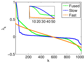
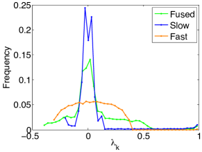
Figure 8: The eigenvalues $\lambda_{k}$ of the matrix $\mathbf{D}^{-1/2}\mathbf{W}\mathbf{D}^{-1/2}$ associated with the fused (green), slow (blue), and fast (orange) graphs. Left: $\lambda_{k}$ as a function of $k$; right: histogram of the $\lambda_{k}$.

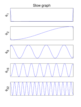
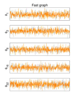
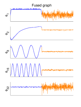
Figure 9: The eigenvectors $\{\phi_{1},\phi_{2},\phi_{8},\phi_{16},\phi_{32}\}$ associated with the slow (left), fast (center), and fused (right) graphs. Right: the large amplitude of the eigenvectors $\phi_{k}$ on the first half of vertices (blue) belonging to the slow subgraph leads to a larger separation between the fast and slow subgraphs when truncating the commute time expansion.

conclude that the slow subgraph has the largest influence on the first few (small $k$) eigenvalues $\lambda_{k}$ of the fused graph.

The eigenvectors of the fused graph and their impact on the commute time

The transition exhibited in the spectrum of the fused graph can also be detected in the corresponding eigenvectors $\phi_{k}$. Figure 9 shows the eigenvectors $\{\phi_{1},\phi_{2},\phi_{8},\phi_{16},\phi_{32}\}$ corresponding to the three graph models. The first eigenvector $\phi_{1}$ has entries equal to the square root of the stationary distribution, $\phi_{1}(\mathbf{x}_{n})=\sqrt{\pi_{n}}$, and is not used in the expansion of the commute time (7). As expected, the random walk spends most of its time inside the slow subgraph of the fused graph, as indicated by the larger values of $\phi_{1}$ for the first (blue) $N/2$ vertices (see Figure 9-right). The eigenvectors $\{\phi_{2},\phi_{8},\phi_{16}\}$ of the fused graph exhibit large amplitude oscillations over the vertices belonging to the slow subgraph (first half – shown in blue – of the plots in Figure 9-right), which resemble those found in the eigenvectors associated with the slow graph (Figure 9-left). As $k$ increases, the eigenvectors $\phi_{k}$ of the fused graph become more and more similar to the eigenvectors of the fast graph.

The impact of the eigenvectors $\phi_{k}$ on the commute time on the fused graph can be analyzed by estimating the size of the terms

$$\frac{1}{1-\lambda_{k}}\left(\frac{\phi_{k}(\mathbf{x}_{n})}{\sqrt{\pi_{n}}}-\frac{\phi_{k}(\mathbf{x}_{m})}{\sqrt{\pi_{m}}}\right)^{2}$$ (22)

in the spectral expansion (7) of the commute time $\kappa$. We claim that $\kappa(\mathbf{x}_{n},\mathbf{x}_{m})$ will be small if both vertices $\mathbf{x}_{n}$ and $\mathbf{x}_{m}$ are in the fast subgraph, and that $\kappa$ will be large if either vertex is in the slow subgraph.

We can first estimate the size of $\phi_{k}(\mathbf{x}_{n})/\sqrt{\pi_{n}}-\phi_{k}(\mathbf{x}_{m})/\sqrt{\pi_{m}}$. We observe that the eigenvectors $\phi_{k}$ for small values of $k$ have large amplitude oscillations on vertices belonging to the slow subgraph, but are relatively constant on the fast subgraph (see Figure 9-right). Therefore, for small values of $k$, each term (22) will be small when $\mathbf{x}_{n}$ and $\mathbf{x}_{m}$ both belong to the fast subgraph (we also have $\pi_{n}\approx\pi_{m}$ when two vertices belong to the same subgraph). Conversely, these terms will be large when either $\mathbf{x}_{n}$ or $\mathbf{x}_{m}$ belongs to the slow subgraph. While this analysis of the size of the terms (22) only holds for small values of $k$, it turns out that these are the terms that have the largest influence in the expansion of the commute time (7). Indeed, the spectrum of the fused graph decays slowly, and therefore the first few coefficients $(1-\lambda_{k})^{-1}$ in the commute time expansion (7) are much larger than the remainders, and therefore the terms (22) for small values of $k$ will provide the largest contribution in the expansion of the commute time.

We conclude that $\kappa(\mathbf{x}_{n},\mathbf{x}_{m})$ is small when $\mathbf{x}_{n}$ and $\mathbf{x}_{m}$ belong to the fast subgraph, and $\kappa(\mathbf{x}_{n},\mathbf{x}_{m})$ is large when either vertex is in the slow subgraph. Furthermore, we expect that this difference will be further magnified if we replace the exact expansion of $\kappa$ in (7) by an approximation that only includes the first few values of $k$.

The truncated spectral expansion of the commute time increases the contrast between the slow and fast subgraphs

We finally come to the heart of the section: the numerical computation of the average approximate commute time defined by

$$\kappa^{\prime}=\frac{2}{N(N-1)}\sum_{n<m}\|\Phi(\mathbf{x}_{n})-\Phi(\mathbf{x}_{m})\|^{2}.$$ (23)

Because of (11), we expect that $\kappa^{\prime}$ will be close to the true commute time $\kappa$. We compute $\kappa^{\prime}$ for the three graphs: slow, fast and fused. We generated 25 realizations of the fast and fused graphs, and we estimated the expected commute time with the sample mean, given by $\kappa^{\prime}$ in (23).

Figure 10-A displays $\kappa^{\prime}_{\mathcal{F}}/\kappa^{\prime}_{\mathcal{S}}$ as a function of the number of terms $d^{\prime}$ used in the embedding (12), for several values of the number of vertices $N$, for the slow and fast graphs. Our theoretical analysis of $\kappa_{\mathcal{F}}/\kappa_{\mathcal{S}}$, performed in Corollary 5.8, is only valid for large values of $N$. Nevertheless, our numerical simulations indicate that for very low values of $N$, $\kappa_{\mathcal{F}}$ is already smaller than $\kappa_{\mathcal{F}}$, since all ratios are below one (see Figure 10-A). Furthermore, we see that this ratio is even smaller for smaller values of $d^{\prime}$. We observe similar results when the commute times $\kappa^{\prime}_{\mathcal{S}}$ and $\kappa^{\prime}_{\mathcal{F}}$ are computed within the slow the fast subgraphs of the fused graph (see

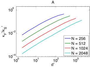
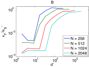
Figure 10: $\kappa^{\prime}_{\mathcal{F}}/\kappa^{\prime}_{\mathcal{S}}$ as a function of the dimension $d^{\prime}$ of the embedding $\Phi$, for several values of the number of vertices $N$. Left: slow $\mathcal{S}$ and fast $\mathcal{F}$ graphs separately; right: slow and fast subgraphs in the fused graph $\Gamma^{\ast}$.

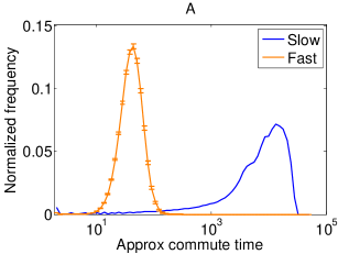
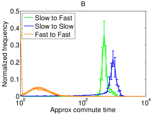
Figure 11: Histogram of $\kappa^{\prime}$. Left: slow graph $\mathcal{S}$ and fast graph $\mathcal{F}$. Right: $\kappa^{\prime}$ for the three types of transition between the subgraphs of the fused graph $\Gamma^{\ast}$. Note the logarithmic scale on the horizontal axes.

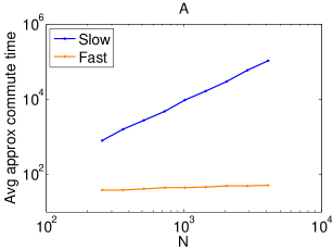
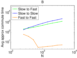
Figure 12: $\kappa^{\prime}$ as function of $N$. Left: slow graph $\mathcal{S}$ and fast graph $\mathcal{F}$. Right: $\kappa^{\prime}$ for the three types of transition between the subgraphs of the fused graph $\Gamma^{\ast}$.

Figure 10-B). These results confirm that the embedding $\Phi$ will further concentrate the vertices of the fast graph if $d^{\prime}$ is chosen to be much smaller than $N$. We have observed experimentally that choosing $d^{\prime}\approx\ln(N)$ leads to the smallest ratio of averages, not only on the graph models, but also on the general patch-graphs studied in section 6.

The enslaving of the fused graph by the slow graph is clearly shown in Figure 11-B, where the normalized histogram of $\kappa^{\prime}$ is shown for the three types of transition between the subgraphs of the fused graph $\Gamma^{\ast}$: slow $\rightarrow$ slow, fast $\rightarrow$ fast, and slow $\rightarrow$ fast. The histogram of the slow $\rightarrow$ fast transition is very similar to the histogram of the slow $\rightarrow$ slow transition, clearly indicating that once the random walk is trapped in the slow subgraph, the presence of the fast subgraph does not help the random walk escape from the slow graph. We also notice that the average of $\kappa^{\prime}$ for the fast $\rightarrow$ fast transition is roughly two orders of magnitude smaller than the average of $\kappa^{\prime}$ for the slow $\rightarrow$ slow, or slow $\rightarrow$ fast transitions. In addition, the variance of each distribution is small enough to limit the overlap between the distributions.

Figure 12 displays $\kappa^{\prime}$ as a function of the number of vertices $N$, where $d^{\prime}=\ln N$. Again, this result confirms that the asymptotic analysis of the ratio $\kappa_{\mathcal{F}}/\kappa_{\mathcal{S}}$, performed in Corollary 5.8, actually holds for very small values of $N$. Indeed, whether the slow and fast graphs are considered separately (Figure 12-A), or are the components of the fused graph (Figure 12-B), the ratio $\kappa_{\mathcal{F}}/\kappa_{\mathcal{S}}\rightarrow 0$ (note the logarithmic scale). It is important to bear in mind that when analyzing images, $N$ is typically of the order of $10^{6}$ and therefore our theoretical analysis will hold without any difficulty. Lastly, we again note in Figure 12-B that the transitions slow $\rightarrow$ fast in the fused graph have the same dynamics as the transition slow $\rightarrow$ slow.

5.5 Summary of the experiments

We have confirmed experimentally that embedding the fused graph using $\Phi$ shrinks the mutual distance between vertices of the fast subgraph, effectively concentrating these vertices closer to one another. As a result, the embedding helps divide the fused graph into the slow and the fast subgraphs by concentrating the vertices of the fast subgraph away from the vertices of the slow subgraph. Our analysis of the embedding is based on the fact that $\Phi$ approximately preserves the commute time measured on the fused graph. Furthermore, we have demonstrated that a truncated version of the commute time, $\kappa^{\prime}$, is even more conducive to identifying vertices of the fast subgraph of the fused graph.

The implication of these results is that the embedding of the true patch-graph $\Gamma$ using $\Phi$ will concentrate the “anomalous” patches, which contain rapid changes in the signal, away from the baseline patches. This concentration of the fast anomalous patches happens for values of the embedding dimension $d^{\prime}$ that are of the order of $\ln(N)$: this choice of $d^{\prime}$ results in a low-dimensional embedding of the patch-graph. Because the fast patches are more clustered after embedding, their detection – for the purpose of detection of anomalies, classification, or segmentation – will become much easier. Finally, we note that our theoretical analysis can be extended to a more general context where patches are replaced by a vector of local features extracted from elements of a large dataset. The only requirement is that the graph of features exhibit a geometry similar to the fused graph $\Gamma^{\ast}$.

6 Numerical experiments with synthetic signals

In this section we validate our theoretical results using synthetic signals. Each signal is the realization of a stochastic process with a prescribed autocorrelation function. We study two types of stochastic processes: one that generates signals that transition from low to high local frequency, and a second one that yields signals with varying local smoothness. We argue that these signals embody the types of local changes that are of fundamental importance in many areas of image processing. For both classes of signals, we embed the patch-sets using $\Phi$ in (12). We study the property of the embedding by quantifying the average commute time $\kappa^{\prime}$, defined in (23) between fast

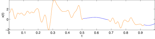
Figure 13: A realization of the time-frequency model. The low frequency portion ($\beta_{\mathcal{S}}=8$) is shown in blue; the high frequency portion ($\beta_{\mathcal{F}}=256$) is shown in orange. There are four subintervals ($\mu=3$).

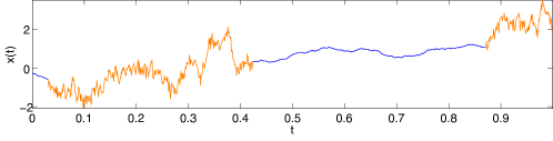
Figure 14: A realization of the local regularity model. The smooth portion ($H_{\mathcal{S}}=0.9$) is shown in blue; the irregular portion ($H_{\mathcal{F}}=0.3$) is shown in orange. There are four subintervals ($\mu=3$).

and slow patches, and we compare the numerical results with the theoretical predictions given in section 5.

6.1 The signals

We consider two types of models: a time-frequency signal model and a local regularity signal model. Each model is characterized by an autocorrelation function. The autocorrelation function can be modified using a parameter that controls the local frequency, or the local regularity of the signal. We partition the interval $[0,1]$ into subintervals over which the autocorrelation parameter is kept constant. The parameter alternates between two different values creating subintervals of alternating local frequency, or alternating local regularity. The number of alternations is chosen randomly according to a homogeneous Poisson process with intensity $\mu$: there are on the average $\mu+1$ subintervals. A simpler version of this model has been used in [13] to mimic the presence of edges in images. Unlike the model used in [13], we adjust the signal defined on each subinterval so that the result is continuous on $[0,1]$. In all experiments that we report here we use $\mu=3$. The autocorrelation function associated with the time-frequency signal model is given by

$$\E(x(t)\overline{x(t+\tau)}=2\left(\frac{1+\cos\left(2\pi\tau\right)}{2}\right)^{\beta}-1,$$ (24)

where $\tau\in[0,1)$, $\beta\geq 0$. As the autocorrelation parameter $\beta$ increases, the range of frequencies present in the signal also increases. Figure 13 displays a realization of this model where the signal’s covariance parameter alternates four times between $\beta_{\mathcal{S}}=8$, and $\beta_{\mathcal{F}}=256$. See appendix C for more on generating a signal from the time-frequency signal model. The autocorrelation function associated with the local regularity signal model is equal to that of fractional Brownian motion, given by

$$\E(x(\tau_{1})\overline{x(\tau_{2})})=\frac{1}{2}\big{(}|\tau_{1}|^{2H}+|\tau_{2}|^{2H}-|\tau_{2}-\tau_{1}|^{2H}\big{)},$$ (25)

where $H$ is the Hurst parameter. As $H$ decreases, the local regularity decreases. A realization of this model is shown in Figure 14 where the signal’s covariance parameter alternates four times between $H_{\mathcal{S}}=0.9$ and $H_{\mathcal{F}}=0.3$. We use the method described in [1] to generate the fractional Brownian motion.

6.2 Embedding the patch-graph

For each realization of a specific signal model, we construct a patch-set of $N=1024$ maximally overlapping patches. The patch size is given by $d=32$ for the time-frequency model, and $d=16$ for the local regularity model. We compute the embedding $\Phi$ (12) and keep $d^{\prime}$ eigenvectors $\phi_{k}$. Figure 15 shows the patch-set associated with the realization of the time-frequency signal displayed in Figure 13 before (left) and after (right) embedding. The scatterplot before embedding is computed using the first three principal components. Figure 16 shows the patch-set associated with the realization of the local regularity signal displayed in Figure 14 before (left) and after (right) embedding. The fast patches of the time-frequency signal are the orange patches extracted from the high frequency segments. The slow patches are the blue patches extracted from the low frequency sections. Similarly, the fast patches of the local regularity signal are the orange patches extracted from the irregular segments, and the slow patches are the blue patches extracted from the smooth sections. For both signals, the fast patches are scattered across the space before embedding. After embedding, the fast patches are aligned along smooth curves. This visual impression is confirmed by computing the mutual distance between patches after embedding, $\|\Phi(\mathbf{x}_{n})-\Phi(\mathbf{x}_{m})\|$. In principle, we should report the value of the Lipschitz ratio

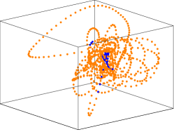
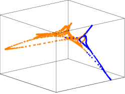
Figure 15: Patch-set of the time-frequency signal (see Figure 13) before (left) and after (right) embedding. The color-code matches the color used in the plot of the signal: blue = low frequency, orange = high frequency.

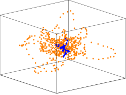
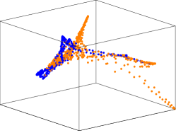
Figure 16: Patch-set of the local regularity signal (see Figure 14) before (left) and after (right) embedding. The color-code matches the color used in the plot of the signal: blue = smooth, orange = irregular.

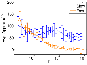
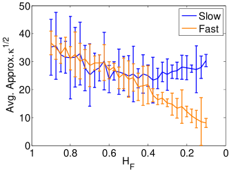
Figure 17: $\sqrt{\kappa^{\prime}}$ for slow (blue) and fast patches (orange) for the time-frequency model (left) and the local regularity model (right) as a function of the “roughness” of the fast patches. The slow patches were generated using $\beta_{\mathcal{S}}=8$ (left) and $H_{\mathcal{S}}=0.9$ (right).

$\|\Phi(\mathbf{x}_{n})-\Phi(\mathbf{x}_{m})\|/\|\mathbf{x}_{n}-\mathbf{x}_{m}\|$ to quantify the contraction experienced through the mapping $\Phi$. However, we have noticed that because the mutual distances $\|\mathbf{x}_{n}-\mathbf{x}_{m}\|$ between fast patches is always large (as explained in section 3), the Lipschitz ratio ends up being always small for fast patches. Therefore studying the size of the Lipschitz ratio associated with $\Phi$ does not reveal whether the map concentrates the fast patches or not, but only indicates that the sampling of the fast patches (in the patch-set) is coarse. For this reason we prefer to study how $\|\Phi(\mathbf{x}_{n})-\Phi(\mathbf{x}_{m})\|$ varies for pairs of slow and fast patches. Based on our theoretical analysis, we expect that after the embedding the mutual distance between fast patches will becomes much shorter than the mutual distance between slow patches.

We point out that the eigenvectors $\phi_{k}$ used in the embedding $\Phi$ (12) are designed to have, on average, small gradients (as measured along edges of the graph). Indeed, these eigenvectors are also the eigenvectors of the graph Laplacian [11], and therefore minimize a Rayleigh ratio that quantifies the average norm of the gradient of $\phi_{k}$. Thus, if we further restricted our computation of the commute times inside each subset of fast and slow patches to only those patches that were connected by an edge in the graph, we would expect to see smaller values and little dependence on whether or not the patch was fast or slow. However, since our theoretical analysis of section 5 is based on the average commute time between all vertices belonging to the fast or slow graph models, we choose to compute the commute times between all patches, not just between patches that are connected with an edge.

For each signal model, we compute the square root of the average approximate commute time

$$\sqrt{\kappa^{\prime}}=\sqrt{\frac{2}{N(N-1)}\sum_{n<m}\|\Phi(\mathbf{x}_{n})-\Phi(\mathbf{x}_{m})\|^{2}}.$$ (26)

for pair of patches $\mathbf{x}_{n},\mathbf{x}_{m}$ that are either both fast, or both slow patches. We study how $\kappa^{\prime}$ varies as a function of the autocorrelation parameter that controls how irregular the fast patches are. $\kappa^{\prime}$ was computed using ten realizations of each signal model. The slow patches were generated using $\beta_{\mathcal{S}}=8$ and $H_{\mathcal{S}}=0.9$. As before, we used $N=1024$ and $d=32$ for the time-frequency model and $d=16$ for the local regularity model. We observed that the overall shapes of the curves in (17) is invariant under variation of the parameters (as along as the ratio of the patch length to the average subinterval length remains less than 10%). The dimension $d^{\prime}$ of the embedding used to compute $\kappa^{\prime}$ was chosen so that $(1-\lambda_{k})^{-1}<0.1(1-\lambda_{2})^{-1}$, for all $k>d^{\prime}+1$. Figure 17 shows $\sqrt{\kappa^{\prime}}$ as a function of the frequency parameter (left), and smoothness parameter (right). We note that as the signal exhibits more rapid, local changes (increasing $\beta_{\mathcal{F}}$, or decreasing $H_{\mathcal{F}}$), the associated fast patches are increasingly concentrated (smaller $\|\Phi(\mathbf{x}_{n})-\Phi(\mathbf{x}_{m})\|$) through the parametrization. These experiments confirm that the theoretical analysis can be applied to the true patch-set constructed from realistic signals.

7 Discussion

Using realistic graph models, probabilistic arguments, and the connection between the commute time of random walks on graphs and the embedding (12), we provided a theoretical explanation for the success of the methods that analyze and process images based on graphs of patches. Our results establish that the embedding of the patch-graph of an image based on the commute time between vertices of the graph reveals the presence of patches containing rapid changes in the underlying signal or image by concentrating these patches close to one another while leaving the patches extracted from the slowly changing portions of the signal organized along low-dimensional structures.

7.1 Parameter selection

7.1.1 Choosing the patch size

In this work we are interested in the local behavior of the image, and therefore $d$ should remain of the order of what we consider to be the local scale. We also note that as $d$ becomes large, the number of available patches ($N/d$) becomes smaller, making the estimation of the geometry of the patch-set more difficult, since patches now live in high-dimension. Another consequence of the “curse of dimensionality” is that the distance between patches becomes less informative for large values of $d$. If the original signal is oversampled with respect to the true physical processes at stake, then one can coarsen the sampling of the patch-set in the image domain. In practice, it would be more advisable to coarsen the underlying continuous patch-set, which is a nontrivial question.

7.1.2 Choosing edge weights

In general, two principles guide the choice of edge weights in the patch-graph. On the one hand, patches that are very close should be connected with a large weight (short distance), while patches that are faraway should have a very small weight along their mutual edge. This principle is equivalent to the idea of only trusting local distances in $\mathbb{R}^{d}$. Such a requirement is intuitively reasonable if we assume that the patch-set represents a discretization of a nonlinear manifold in $\mathbb{R}^{d}$. In this situation, we know that when the points on the manifold are very close to another, the geodesic distance is well approximated by the Euclidean distance. Conversely, because of the presence of curvature, the Euclidean distance is a poor approximation to the geodesic distance on the manifold when points are far apart. Because the only information available to us is the Euclidean distance between patches, we should not trust large Euclidean distances.

On the other hand, as observed in Section 3, the fast patches, which contain rapid changes, are all very far apart (large $\rho^{2}(\mathbf{x}_{n},\mathbf{x}_{m})$). Therefore the probability that the random walk escapes the fast patch $\mathbf{x}_{n}$ and jumps to a different patch $\mathbf{x}_{m}$, which is given by

$$\frac{w_{n,m}}{\sum_{l}w_{n,l}}=\frac{e^{\displaystyle-\rho^{2}(\mathbf{x}_{n},\mathbf{x}_{m})/\sigma^{2}}}{\sum_{l}w_{n,l}},$$

is always much smaller than the probability of staying at $\mathbf{x}_{n}$, which is given by

$$\frac{1}{\sum_{l}w_{n,l}}.$$

In order to avoid that the random walk be trapped at each node $\mathbf{x}_{n}$, we “saturate” the distance function by choosing $\sigma$ to be very large. In this case, for all the nearest neighbors $\mathbf{x}_{m}$ of $\mathbf{x}_{n}$, we have $w_{n,m}\approx 1$, and the transition probability is the same for all the neighbors, $\mathbf{P}_{n,m}\approx 1/\nu$. This choice of $\sigma$ promotes a very fast diffusion of the random walk locally. We note that choosing a large $\sigma$ may be avoided if self-connections are not enforced (i.e. $w_{n,n}=0$). However, self-connections are a necessary technical requirement to prove that the Markov process is aperiodic, which is required to prove the equality (8) [14].

We note that choosing $\sigma$ to be very large does not entirely obliterate the information provided by the mutual distance between patches, measured when patches are projected on the sphere with $\rho(\mathbf{x}_{n},\mathbf{x}_{m})$, (3). Indeed, $\rho(\mathbf{x}_{n},\mathbf{x}_{m})$ is used to select the nearest neighbors of each patch, and therefore allows us to define a notion of a local neighborhood around each patch. Choosing $\sigma$ to be very large forces a very fast diffusion within this neighborhood, irrespective of the actual distances $\rho(\mathbf{x}_{n},\mathbf{x}_{m})$. Alternatively, we could consider choosing $\sigma$ to vary adaptively from one neighborhood to another. The parameter $\sigma$ could be small when patches are extremely close to one another, while $\sigma$ could be large when the patches are at a large mutual distance of one another. This notion is the foundation of the self-tuning weight matrix, which adjusts its weights based on a point’s local neighborhood [30].

7.2 Extensions and generalizations

In general, the patch-set of an image consists of more than two homogeneous subsets. For example, one could partition an image patch-set into uniform patches, edge patches, and texture patches. Our experience [40] with a generalization of the time-frequency signal model (section 6) indicates that we can still separate the patches when the signal is composed of up to four different local behaviors (specified by four different values of the parameter in the autocorrelation function). Another extension of this work involves the embedding of a patch-set constructed from a library of images. Recent studies [26] indicate that high-contrast patches extracted from optical images organize themselves around 2-dimensional smooth sub-manifold ([8]). This idea has also been exploited to construct dictionaries that lead to very sparse representations of images (e.g. [18], and references therein). Finally, we note that our results about the embedding of the slow (14), fast (5.2), and the fused graph (5.3) are very general and can be applied to datasets [9] where the corresponding graph exhibits a similar structure. For instance, one could imagine using this idea to study social networks, where the concept of cliques would correspond to fast subgraphs.

7.3 Related work

The concept of patches has proven extremely useful in many areas of image analysis: texture analysis/synthesis [28], image completion [31, 44], super-resolution [34], and denoising [5, 7, 22, 24, 33, 37, 38, 44]. While these references do not explicitly construct a patch-graph, these works all compute distances between patches, and use the nearest neighbors of each patch to analyze and process patches. Recent works on the analysis of time-series also use patches and construct networks of patches [4, 25, 43]. All these references provide experimental evidence for the success of working on image (or signal) patches.

In this work, we provide a theoretical justification for this experimental success. We study the effect of the embedding $\Phi$ (12) on the organization of the patch-set. Our analysis assumes that there exists a natural partition of the patch-set into two classes: patches extracted from the smooth baseline and patches that contain sudden local changes of the image intensity or signal value. It is interesting to compare and contrast our work to the work of Singer, Shkolnisky, and Nadler [37] who provide a different theoretical explanation for the success of patch-based denoising algorithms. The authors in [37] treat the matrix $\mathbf{P}$ as a filter, which acts on an $N$-dimensional column-vector-representation of the signal or the image. Each multiplication of the probability distribution by $\mathbf{P}$ is interpreted as the evolution of the diffusion process on the patch-graph over a time-step of duration $\sigma$. The results in [37] rely on the convergence of a properly normalized version of $\mathbf{P}$ toward the backward Fokker-Planck operator. The authors can compute the eigenfunctions of the operator when the signal is either a one-dimensional constant function perturbed by Gaussian noise, or a one-dimensional step function also contaminated by Gaussian noise.

In contrast, our analysis is based on the analysis of the commute time on graphs that epitomize the patch-graph constructed from two classes of patches. In addition, we need not assume that the image is piece-wise constant. In fact, our experiments demonstrate that our analysis can be applied to detect many different types of anomalies: changes in the local frequency content, changes in local regularity, etc. Furthermore, our theoretical analysis holds for finite values of the number of patches $N$. It is interesting to note that Singer et al. study the mean first-passage time between patches extracted from the noisy step function. The mean first-passage time is derived from the hitting time, which is used to define the commute time. The authors in [37] use an energy argument to explain the existence of a large mean first-passage time between patches extracted from either side of the step function’s discontinuity. They argue that a high density of patches is associated with a lower potential energy, and consequently it will take longer for a random process to exit the well with such a low potential. Finally, our results are not limited to patches of size $d=1$, as are the results in [37].

The energy argument in [37] adds an interesting interpretation to our analysis. Following this perspective, the slow patches can be interpreted as points sampled from a probability density function $P$ defined on $\mathbb{R}^{d}$ with a support that is defined along a low-dimensional manifold. This localization leads to a potential $U=-\log P$ with a deep and narrow well, from which the random walk cannot escape. This argument agrees with our findings that the average commute time between slow patches is very large, and thus, the random walk spends considerably more time in the slow subgraph before being able to reach a patch that is temporally faraway.

From a more general perspective, this work presents an investigation into the diffusion process on the graphs models presented in Section 5.2. Our work is thus related to a large body of work on the analysis of complex and random networks using first-passage time (e.g. [15] and references therein). This area if usually motivated by physical problems such as transport in disordered media, neuron firing, or energy flow on power-grids instead of applications in signal processing.

7.4 Open questions

While we obtained estimates for the average commute time on the fast and slow graph models considered separately, it would be desirable to obtain similar estimates on the fused graph. At the moment, our analysis of the fused graph relies on numerical simulations. We are also aware of a small discrepancy in the upper bound on $\kappa_{\mathcal{F}}$: this bound is increasing with $L$. In fact we expect that the commute time on $\mathcal{F}(N,p)$ should decrease as $p$, and therefore $L$, increases. The reason for this apparent inconsistency is that the proof of (20) relies on a loose upper bound for the effective resistance between two vertices, which is provided by the geodesic distance on the graph [10]. This is not a tight inequality on a graph such as $\mathcal{F}(N,p)$. A more effective inequality, which could improve the upper bound (20), relies on the computation of the distribution of the number of paths $s$ of length at most $l$ between the two vertices. We could then use the fact that the commute time is bounded from above by a constant times the ratio $l/s$ [10], which would decrease the upper bound in (20).

Appendix A The connectedness of the fast graph

It is necessary that the fast graph $\mathcal{F}(N,p)$ be connected to be able to apply the spectral decomposition of the commute time. To ensure that the probability of $\mathcal{F}(N,p)$ being disconnected will vanish as $N$ gets large, we must choose $Np>\log N$ [17]. Since $p$ is defined as a function of $L$ in (16), any requirement on $p$ ultimately constrains $L$. First, because the maximum degree of a vertex in $\mathcal{S}(N,L)$ is $2L+1$, according to (14), we require

$$2L+1\leq N.$$

Manipulation of this inequality leads to

$$\frac{L+1}{N}\leq\frac{1}{2}+\frac{1}{2N}.$$

We assume that $N\geq 2$, so that

$$\frac{L+1}{N}\leq\frac{3}{4}.$$

It follows that

$$\left(2-\frac{L+1}{N}\right)\geq\frac{5}{4}>1.$$

Therefore, rewriting (16) and using the last inequality we have

$$p=\frac{L}{N-1}\left(2-\frac{L+1}{N}\right)>\frac{L}{N}\left(2-\frac{L+1}{N}\right)>\frac{L}{N}.$$

Therefore, choosing $L=c\log N$ for some $c>1$ ensures that $Np>\log N$, and consequently, the probability of $\mathcal{F}(N,p)$ being disconnected approaches zero as $N$ approaches infinity.

Appendix B Bounding the commute times in the graph models

B.1 Proof of the lower bound on the average commute time in the slow graph

In order to compute a lower bound on the average commute time, we consider a fixed pair of vertices in the slow graph, $\mathbf{x}_{n_{0}}$ and $\mathbf{x}_{m_{0}}$, and compute a lower bound on the commute time $\kappa(\mathbf{x}_{n_{0}},\mathbf{x}_{m_{0}})$. We can then compute the average of this lower bound over all the pairs of vertices. To obtain the lower bound on $\kappa(\mathbf{x}_{n_{0}},\mathbf{x}_{m_{0}})$ we use a standard tool to obtain lower bounds on commute time: the Nash-Williams inequality [29]. The Nash-Williams inequality is usually formulated in terms of electrical networks. We prefer to present an equivalent formulation that is directly adapted to our problem. We first introduce the concept of edge-cutset.

Definition B.1.

Let $V_{1}$ and $V_{2}$ be two disjoint sets of vertices. A set of edges $E$ is an edge-cutset separating $V_{1}$ and $V_{2}$ if every path that connects a vertex in $V_{1}$ with a vertex in $V_{2}$ includes an edge in $E$.

Given a weighted graph, which may contain loops, we define a random walk with the probability transition matrix $\mathbf{P}_{n,m}=\mathbf{W}_{n,m}/\mathbf{D}_{n,n}$. Let $\mathbf{x}_{m_{0}}$ and $\mathbf{x}_{n_{0}}$ be two vertices. The commute time between vertices $\mathbf{x}_{m_{0}}$ and $\mathbf{x}_{n_{0}}$, $\kappa(\mathbf{x}_{m_{0}},\mathbf{x}_{n_{0}})$ satisfies the following lower bound.

Lemma B.2 (Nash-Williams).

If $\mathbf{x}_{m_{0}}$ and $\mathbf{x}_{n_{0}}$ are distinct vertices in a graph that are separated by disjoint edge-cutsets $E_{k},k=1,\ldots$, then

$$V\;\sum_{k}\left[\sum_{\{\mathbf{x}_{n},\mathbf{x}_{m}\}\in E_{k}}w_{n,m}\right]^{-1}\leq\kappa(\mathbf{x}_{m_{0}},\mathbf{x}_{n_{0}})\qquad\text{where $\{\mathbf{x}_{m},\mathbf{x}_{n}\}$ is an edge in the cutset $E_{k}$},$$ (27)

and where the volume of the graph is defined by $V=\sum_{i=1}^{N}\sum_{j=1}^{N}w_{i,j}$.

We now exhibit a sequence of edge-cutsets in the slow graph. We refer to Figure 18 for the construction of the cutsets. We define the first cutset $E_{1}$. If $m_{0}<L$, then $E_{1}$ needs a little more attention and is defined as the set of $L$ edges $\{\mathbf{x}_{i},\mathbf{x}_{j}\}$, where $i$ and $j$ are defined by

$$\begin{cases}i=1,\ldots,m_{0},\\ j=m_{0}+1,\ldots,L+i.\end{cases}$$ (28)

The edge-cutset $E_{1}$ is shown in the Figure 18 for $m_{0}=1$ (left) and $m_{0}=2$ (center), for $L=3$. The removal of this set of edges prevents $\mathbf{x}_{m_{0}}$ from being connected to $\mathbf{x}_{n_{0}}$. Indeed, the self loop on the diagonal (green entry) does not allow the random walk to move toward $\mathbf{x}_{n_{0}}$. This can be also be visualized in Figure 19, where $E_{1}$ is the leftmost set of edges that connect $\mathbf{x}_{m_{0}}$ to that part of the graph that is connected to $\mathbf{x}_{n_{0}}$. The sum of edge weights in $E_{1}$ is at most $L(L+1)w_{\mathcal{S}}/2$. If $m_{0}\geq L$, then $E_{1}$, is defined as the other generic edge-cutsets.

We now define the generic edge-cutsets $E_{k}$ as the set of $L(L+1)/2$ edges $\{\mathbf{x}_{i},\mathbf{x}_{j}\}$ such that

$$\begin{cases}i=m_{0}+1+(k-2)L,\ldots,m_{0}+(k-1)L,\\ j=m_{0}+1+(k-1)L,\ldots,L+i.\end{cases}$$ (29)

As seen in Figure 18-right for $k=3$, setting the entries of $E_{3}$ to zero disconnects the upper and lower part of the submatrix $\mathbf{W}(m_{0}:n_{0},m_{0}:n_{0})$, thereby isolating $\mathbf{x}_{m_{0}}$ and $\mathbf{x}_{n_{0}}$. Alternatively, we also see in Figure 19 that any path from $\mathbf{x}_{m_{0}}$ to $\mathbf{x}_{n_{0}}$ needs to go through $E_{3}$. Each edge-cutset $E_{k},k\geq 2$ is a triangle with a height of size $L$. Therefore, after creating $E_{1}$, we can fit $\left\lfloor\frac{n_{0}-(m_{0}+1)+1}{L}\right\rfloor$ such cutsets between $\mathbf{x}_{m_{0}+1}$ and $\mathbf{x}_{n_{0}}$. The sum of the weights along the edges of each cutset $E_{k},k=2,\ldots$ is given by $L(L+1)w_{s}/2$. In addition, the sum of edge weights in the first cutset $E_{1}$ is at most $L(L+1)w_{s}/2$. Putting everything together, the computation of the lower bound using the Nash-Williams Lemma yields

$$\begin{split}V\sum_{k}&\left[\sum_{\{n,m\}\in E_{k}}w_{n,m}\right]^{-1}\\ &\geq\left[N(2L+1)-L(L+1)\right]w_{s}\left(\left\lfloor\frac{(n_{0}-m_{0})}{L}\right\rfloor\frac{2}{L(L+1)w_{s}}+\frac{2}{L(L+1)w_{s}}\right)\\ &\geq\frac{\left[N(2L+1)-L(L+1)\right]}{L(L+1)}\left(2\left(\frac{n_{0}-m_{0}}{L}-1\right)+2\right)\\ &\geq\frac{\left[N(2L+1)-L(L+1)\right]}{L(L+1)}\left(2\frac{n_{0}-m_{0}}{L}\right)\end{split}$$

We can summarize this result in the following lemma.

Lemma B.3.

The commute time between vertices $\mathbf{x}_{n_{0}}$ and $\mathbf{x}_{m_{0}}$ inside $\mathcal{S}(N,L)$ satisfies

$$\kappa(\mathbf{x}_{m_{0}},\mathbf{x}_{n_{0}})\geq\frac{2\left[N(2L+1)-L(L+1)\right]}{L(L+1)}\left(\frac{n_{0}-m_{0}}{L}\right).$$ (30)

Finally, we bound the average commute time in the slow graph. Observe that the slow graph model $\mathcal{S}(N,L)$ has $N-j$ pairs of vertices such that $|m-n|=j$, for $j=1,\ldots,N-1$. Therefore, using the lower bound given in Lemma 30 it follows that

$$\sum_{1\leq m<n\leq N}\kappa(\mathbf{x}_{m},\mathbf{x}_{n})\geq\frac{2\left[N(2L+1)-L(L+1)\right]}{L^{2}(L+1)}\sum_{j=1}^{N-1}(N-j)j$$

But

$$\sum_{j=1}^{N-1}(N-j)j =\left(N\sum_{1}^{N-1}j-\sum_{1}^{N-1}j^{2}\right)=\left(\frac{N^{2}(N-1)}{2}-\frac{N(N-1)}{2}\frac{2N-1}{3}\right)$$

$$=\frac{N(N-1)}{2}\frac{N+1}{3}$$

Dividing both sides by $N(N-1)/2$ and simplifying yields (19).

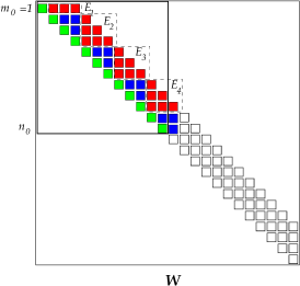
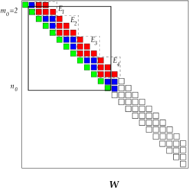
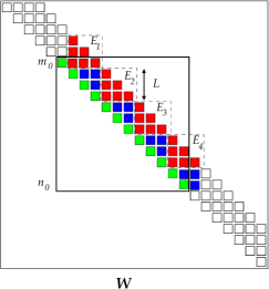
Figure 18: The small squares represent the nonzero entries in the upper triangular portion of the weight matrix $\mathbf{W}$ of $\mathcal{S}(N,L)$. The green entries on the diagonal are the self-loops. The edge-cutsets $E_{k}$ are shown in red for $m_{0}=1$ (left), $m_{0}=2$ (center), and for $m_{0}\geq L$ (right). The submatrix $\mathbf{W}(m_{0}:n_{0},m_{0}:n_{0})$ is also shown.

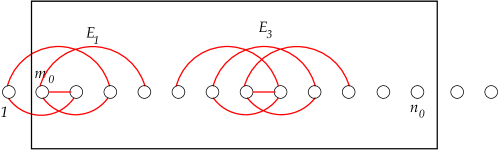
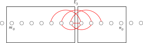
Figure 19: Top: edge-cutsets $E_{1}$ and $E_{3}$. Bottom: any path from $m_{0}$ to $n_{0}$ needs to use an edge of the edge-cutset $E_{3}$.

B.2 Proof of upper bound on the average commute time in the fast graph

Our approach relies on the relationship between electrical networks and random walks on graphs [16]. We begin by introducing the property of interest — the effective resistance — and its relationship to the commute time.

The electrical network perspective

For each pair of vertices $\mathbf{x}_{n}$ and $\mathbf{x}_{m}$ with a non zero weight $w_{n,m}$, we assign the resistance

$$r_{n,m}=\frac{1}{w_{n,m}}$$ (31)

to the edge $\{\mathbf{x}_{n},\mathbf{x}_{m}\}$. We note that if $w_{n,m}=0$, then there is no connection between $\mathbf{x}_{n}$ and $\mathbf{x}_{m}$, and no resistance to consider. Now, consider applying a potential difference, or voltage, across the vertices $\mathbf{x}_{m_{0}}$ and $\mathbf{x}_{n_{0}}$. As a result, some current flows across the resistors (edges) in the electrical network (graph). We may replace the set of resistors across which some current flows by an equivalent, effective resistance, $R_{m_{0},n_{0}}$ that is connected between $\mathbf{x}_{m_{0}}$ and $\mathbf{x}_{n_{0}}$. The effective resistance $R_{m_{0},n_{0}}$ is defined by the voltage necessary to maintain a one-unit current between $\mathbf{x}_{m_{0}}$ and $\mathbf{x}_{n_{0}}$. The main result in [10], is that the commute time between vertices $\mathbf{x}_{m_{0}}$ and $\mathbf{x}_{n_{0}}$ can be expressed as

$$\kappa(\mathbf{x}_{m_{0}},\mathbf{x}_{n_{0}})=VR_{m_{0},n_{0}}.$$ (32)

Taking expectations of both sides of Equation (32) with respect to the process of generating edges and choosing terminals in a fast graph, we obtain

$$\kappa_{\mathcal{F}}=\E(V)\,\E(R)+\operatorname{Cov}(V,R).$$ (33)

Notice that every edge in the fast graph has weight $w_{\mathcal{F}}$. Therefore, $V$ can be expressed as

$$V=\sum_{n=1}^{N}w_{nn}+2\sum_{1\leq m<l\leq N}w_{ml}=w_{\mathcal{F}}N+2w_{\mathcal{F}}\tilde{N},$$ (34)

where $\tilde{N}$ is a binomial random variable representing the number of edges connecting distinct vertices in the fast graph. We now rewrite (33), using (34) and the assumption that $\operatorname{Cov}(V,R)\leq 0$, to obtain

$$\kappa_{\mathcal{F}}\leq w_{\mathcal{F}}\left[N+2\E(\tilde{N})\right]\E(R).$$

Recall that $\tilde{N}$ is distributed as a binomial random variable with parameters $(N(N-1)/2,p)$. Also, the effective resistance between two nodes of a network is at most the geodesic distance between them, $\delta$, scaled by $1/w_{\mathcal{F}}$ [10]. It follows that

$$\kappa_{\mathcal{F}}\leq\left[N(N-1)p+N\right]\E(\delta).$$

The authors [20] give a closed form expression for $\E(\delta)$ on Erdös-Renyi graphs, which we can utilize since the fast graph’s self-connections do not change the geodesic distance. This yields

$$\kappa_{\mathcal{F}}\leq\left[N(N-1)p+N\right]\left[\frac{\log N-\gamma_{e}}{\log((N-1)p+1)}+\frac{1}{2}\right],$$

where $\gamma_{e}\approx 0.5772$ is Euler’s constant. Simplification using (16) gives the desired result.

Remark

Although $\operatorname{Cov}(V,R)\leq 0$ is an assumption, we conjecture that it is always satisfied due to the fact that increasing the number of resistors $M$ in an electrical network with a fixed number of nodes is effectively like adding resistors-in-parallel, and, according to Rayleigh’s Monotonicity Law, adding edges (increasing $M$) can only decrease the effective resistance [16].

Appendix C Generating a random trigonometric polynomial with a specified autocorrelation

Let $z(t)$ represent a random trigonometric polynomial on $[0,1)$ with an autocorrelation function given by

$$C(\tau)=2(\cos(\pi\tau))^{2\beta}-1\hskip 14.45377pt\text{ for }\tau\in\left[-\frac{1}{2},\frac{1}{2}\right),$$ (35)

for some nonnegative integer $\beta$. It follows that we can do a Fourier expansion of $C(\tau)$ to obtain

$$C(\tau)=\sum_{j\in\mathbb{Z}}\hat{C}_{j}e^{2\pi ijt},$$ (36)

where $i=\sqrt{-1}$ and

$$\hat{C}_{j} =\int_{0}^{1}C(\tau)e^{-2\pi ij\tau}d\tau$$

$$=\int_{0}^{1}\left(2^{(1-2\beta)}\left(\sum_{k=0}^{2\beta}\begin{pmatrix}2\beta\\ k\end{pmatrix}e^{2\pi i(\beta-k)\tau}\right)-1\right)e^{-2\pi ij\tau}d\tau$$

$$=2^{(1-2\beta)}\sum_{k=0}^{2\beta}\begin{pmatrix}2\beta\\ k\end{pmatrix}\int_{0}^{1}e^{2\pi i(\beta-k-j)\tau}\,d\tau-\int_{0}^{1}e^{-2\pi ij\tau}\,d\tau$$

$$=\left\{\begin{array}[]{ll}2^{(1-2\beta)}\begin{pmatrix}2\beta\\ \beta\end{pmatrix}-1&\text{if }j=0,\vspace{.05in}\\ 2^{(1-2\beta)}\begin{pmatrix}2\beta\\ \beta-j\end{pmatrix}&\text{if }|j|\leq\beta,\\ 0&\text{if }j>\beta,\end{array}\right.$$

where the second equality follows after expressing cosine with complex exponentials, and applying the binomial theorem.

It is clear that $2\beta$ is the frequency of the fastest sinusoid making up the random signal $z(t)$, and that most of the energy is on average at frequency $\beta$. Let $A_{j}$ and $B_{j}$ be independent and identically distributed Normal random variables with zero mean and unit variance. Define

$$\hat{z}_{j}=\sqrt{\frac{\hat{C}_{j}}{2}}\left(A_{j}+iB_{j}\right).$$

Finally, the signal $z(t)$ is defined as

$$z(t)=\sum_{j\in\mathbb{Z}}\hat{z}_{j}e^{2\pi ijt}.$$

To check that the signal $z(t)$ defined above has the correct autocorrelation, observe that linearity of the expectation, independence and zero mean of the random variables, and the fact that $\hat{C}_{j}=\hat{C}_{-j}$ together imply that

$$\E(z(t) \overline{z(t+\tau)})=\sum_{|j|\leq 2\beta}\sum_{|k|\leq 2\beta}\E\left(\hat{z}_{j}\overline{\hat{z}_{k}}\right)e^{-2\pi ik\tau}e^{2\pi i(j-k)t}$$

$$=\sum_{|j|\leq 2\beta}\sum_{|k|\leq 2\beta}\frac{\sqrt{\hat{C}_{j}\hat{C}_{k}}}{2}\left[\E(A_{j}A_{k})-i\E(A_{j}B_{k})+i\E(A_{k}B_{j})+\E(B_{j}B_{k})\right]e^{-2\pi ik\tau}e^{2\pi i(j-k)t}$$

$$=\sum_{|j|\leq 2\beta}\frac{\hat{C}_{j}}{2}\left[\E(A_{j}^{2})+\E(B_{j})^{2}\right]e^{-2\pi ij\tau}=\sum_{|j|\leq 2\beta}\hat{C}_{j}e^{2\pi ij\tau}.$$

Therefore, referencing (36), it follows that $\E(z(t)\overline{z(t+\tau)})=C(\tau)$.

References

- [1] P. Abry and F. Sellan, The wavelet-based synthesis for fractional Brownian motion proposed by F. Sellan and Y. Meyer, Appl. Comput. Harmon. A., 3 (1996), pp. 377–383.
- [2] M. Belkin and P. Niyogi, Laplacian eigenmaps for dimensionality reduction and data representation, Neural Computations, 15 (2003), pp. 1373–1396.
- [3] O. Bénichou, C. Chevalier, J. Klafter, B. Meyer, and R. Voituriez, Geometry-controlled kinetics, Nature chemistry, 2 (2010), pp. 472–477.
- [4] E.P. Borges, D.O. Cajueiro, and F.S. Andrade, Mapping dynamical systems onto complex networks, The European Physical Journal B - Condensed Matter and Complex Systems, 58 (2007), pp. 469–474.
- [5] S. Bougleux, A. Elmoataz, and M. Melkemi, Local and nonlocal discrete regularization on weighted graphs for image and mesh processing, Intern. J. Comput. Vis., 84 (2009), pp. 220–236.
- [6] P. Bremaud, Markov Chains, Springer Verlag, 1999.
- [7] A. Buades, B. Coll, and J.M. Morel, A review of image denoising algorithms, with a new one, Multiscale Modeling and Simulation, 4 (2005), pp. 490–530.
- [8] G. Carlsson, T. Ishkhanov, V. De Silva, and A. Zomorodian, On the local behavior of spaces of natural images, Intern. J. Comput. Vis., 76 (2008), pp. 1–12.
- [9] F. Cazals, F. Chazal, and J. Giesen, Spectral techniques to explore point clouds in euclidean space, in Nonlinear Computational Geometry, Springer, 2010, pp. 1–34.
- [10] A.K. Chandra, P. Raghavan, W.L. Ruzzo, and R. Smolensky, The electrical resistance of a graph captures its commute and cover times, in Proc. 21st ACM Symposium on Theory of Computing, ACM, 1989, pp. 574–586.
- [11] F. Chung, Spectral Graph Theory, American Mathematical Society, 1997.
- [12] F. Chung, L. Lu Linyuan, and V. Vu, Spectra of random graphs with given expected degrees, P. Natl. Acad. Sci. USA, 100 (2003), pp. 6313–6318.
- [13] A. Cohen and J.P. D’Ales, Nonlinear approximation of random functions, SIAM J. Appl. Math., 57 (1997), pp. 518–540.
- [14] R.R. Coifman and S. Lafon, Diffusion maps, Applied and Computational Harmonic Analysis, 21 (2006), pp. 5–30.
- [15] S. Condamin, O. Bénichou, V. Tejedor, R. Voituriez, and J. Klafter, First-passage times in complex scale-invariant media, Nature, 450 (2007), pp. 77–80.
- [16] P.G. Doyle and J.L. Snell, Random Walks and Electric Networks, ArXiv Mathematics e-prints, (2000). Available from arxiv.org/abs/math/0001057.
- [17] R. Durrett, Random Graph Dynamics, Cambridge, 2007.
- [18] M. Elad, Sparse and Redundant Representations: From Theory to Applications in Signal and Image Processing, Springer Verlag, 2010.
- [19] P. Erdos and A. Renyi, On the evolution of random graphs, Publ. Math. Inst. Hung. Acad. Sci, 5 (1960), pp. 17–61.
- [20] A. Fronczak, P. Fronczak, and J.A. Hołyst, Average path length in random networks, Phys. Rev. E, 70 (2004).
- [21] A. Ghosh, S. Boyd, and A. Saberi, Minimizing effective resistance of a graph, SIAM Rev., 50 (2008), pp. 37–66.
- [22] G. Gilboa and S. Osher, Nonlocal operators with applications to image processing, Multiscale Model. Simul., 7(3) (2008), pp. 1005–1028.
- [23] P.W. Jones, M. Maggioni, and R. Schul, Manifold parametrizations by eigenfunctions of the Laplacian and heat kernels, P. Natl. Acad. Sci. USA, 105 (2008), pp. 1803–1808.
- [24] V. Katkovnik, A. Foi, K. Egiazarian, and J. Astola, From local kernel to nonlocal multiple-model image denoising, Intern. J. Comput. Vis., 86 (2010), pp. 1–32.
- [25] L. Lacasa, B. Luque, F. Ballesteros, J. Luque, and J. Nu no, From time series to complex networks: The visibility graph, P. Natl. Acad. Sci. USA, 105 (2008), pp. 4972–4975.
- [26] A.B. Lee, K.S. Pedersen, and D. Mumford, The nonlinear statistics of high-contrast patches in natural images, Intern. J. Comput. Vis., 54 (2003), pp. 83–103.
- [27] L. Lovász, Random walks on graphs: A survey, in Combinatorics: Paul Erdös is eighty, vol. 2, János Bolyai Math. Soc, 1993, pp. 1–46.
- [28] J. Lu, J. Dorsey, and H. Rushmeier, Dominant texture and diffusion distance manifolds, Computer Graphics Forum, 28 (2009), pp. 667–676.
- [29] R. Lyons and Y. Peres, Probability on trees and networks. In preparation. Available at http://mypage.iu.edu/rdlyons.
- [30] L.Z. Manor and P. Perona, Self-tuning spectral clustering, in Proceedings of the 18th Annual Conference on Neural Information Processing Systems (NIPS’04), 2004.
- [31] H. Mobahi, S. Rao, and Y. Ma, Data-driven image completion by image patch subspaces, in Proc. 27th Conf. on Picture Coding Symposium, IEEE Press, 2009, pp. 241–244.
- [32] P.Bérard, G. Besson, and S. Gallot, Embeddings Riemannian manifolds by their heat kernel, Geometric and Functional Analysis, 4(4) (1994), pp. 373–398.
- [33] G. Peyré, Image processing with non-local spectral bases, Multiscale Model. Simul., 7 (2008), pp. 703–730.
- [34] M. Protter, M. Elad, H. Takeda, and P. Milanfar, Generalizing the nonlocal-means to super-resolution reconstruction, Image Processing, IEEE Transactions on, 18 (2009), pp. 36 –51.
- [35] T. Sauer, J.A. Yorke, and M. Casdagli, Embedology, Journal of Statistical Physics, 65 (1991), pp. 579–616. 10.1007/BF01053745.
- [36] X. Shen and F.G. Meyer, Low-dimensional embedding of fMRI datasets, NeuroImage, 41 (2008), pp. 886 – 902.
- [37] A. Singer, Y. Shkolnisky, and B. Nadler, Diffusion Interpretation of Nonlocal Neighborhood Filters for Signal Denoising, SIAM Journal of Imaging Sciences, 2 (2009), pp. 118–139.
- [38] A. Szlam, M. Maggioni, and R.R. Coifman, Regularization on graphs with function-adapted diffusion processes, Journal of Machine Learning Research, 9 (2008), pp. 1711–1739.
- [39] F. Takens, Detecting strange attractors in turbulence, in Dynamical systems and turbulence, Warwick 1980 (Coventry, 1979/1980), Lecture Notes in Math., 898, Springer, 1981, pp. 366–381.
- [40] K.M. Taylor, The geometry of signal and image patch-sets, PhD thesis, University of Colorado, Boulder, Dept. of Applied Mathematics, June 2011. (available from ecee.www.colorado.edu/fmeyer).
- [41] K.M. Taylor, M.J. Procopio, C.J. Young, and F.G. Meyer, Estimation of arrival times from seismic waves: a manifold-based approach, Geophys. J. Intern., 185 (2011), pp. 435–452.
- [42] S. Vempala, Geometric random walks: A survey, MSRI volume on Combinatorial and Computational Geometry, (2005).
- [43] J. Zhang and M. Small, Complex network from pseudoperiodic time series: Topology versus dynamics, Phys. Rev. Lett., 96 (2006), p. 238701.
- [44] M. Zhou, H. Chen, J. Paisley, L. Ren, G. Sapiro, and L. Carin, Non-parametric Bayesian dictionary learning for sparse image representations, in Advances in Neural Information Processing Systems 22, Y. Bengio, D. Schuurmans, J. Lafferty, C. K. I. Williams, and A. Culotta, eds., 2009, pp. 2295–2303.