Shear and Bulk Viscosities of a Gluon Plasma in Perturbative QCD: Comparison of Different Treatments for the $gg\leftrightarrow ggg$ Process

Abstract

The leading order contribution to the shear and bulk viscosities, $\eta$ and $\zeta$, of a gluon plasma in perturbative QCD includes the $gg\leftrightarrow gg$ (22) process, $gg\leftrightarrow ggg$ (23) process and multiple scattering processes known as the Landau-Pomeranchuk-Migdal (LPM) effect. Complete leading order computations for $\eta$ and $\zeta$ were obtained by Arnold, Moore and Yaffe (AMY) and Arnold, Dogan and Moore (ADM), respectively, with the inelastic processes computed by an effective $g\leftrightarrow gg$ gluon splitting. We study how complementary calculations with 22 and 23 processes and a simple treatment to model the LPM effect compare with the results of AMY and ADM. We find that our results agree with theirs within errors. By studying the contribution of the 23 process to $\eta$, we find that the minimum angle $\theta$ among the final state gluons in the fluid local rest frame has a distribution that is peaked at $\theta\sim\sqrt{\alpha_{s}}$, analogous to the near collinear splitting asserted by AMY and ADM. However, the average of $\theta$ is much bigger than its peak value, as its distribution is skewed with a long tail. The same $\theta$ behavior is also seen if the 23 matrix element is taken to the soft gluon bremsstrahlung limit in the center-of-mass (CM) frame. This suggests that the soft gluon bremsstrahlung in the CM frame still has some near collinear behavior in the fluid local rest frame. We also generalize our result to a general $SU(N_{c})$ pure gauge theory and summarize the current viscosity computations in QCD.

I Introduction

Shear and bulk viscosities, $\eta$ and $\zeta$, are transport coefficients characterizing how fast a system goes back to equilibrium under a shear mode perturbation and a uniform expansion, respectively. In a weakly interacting hot gluon plasma, $\eta$ is inversely proportional to the scattering rate, $\eta\propto 1/\Gamma\propto 1/\alpha_{s}^{2}\ln\alpha_{s}^{-1}$ Arnold:2000dr , where $\alpha_{s}$ is the strong coupling constant. $\zeta$ is suppressed by an additional factor of $\left(T_{\mu}^{\mu}\right)^{2}$, arising from the response of the trace of the energy momentum tensor $\left(T_{\mu}^{\mu}\right)$ to a uniform expansion. Thus, $\zeta$ vanishes when the system is “conformal” or scale invariant. For a gluon plasma, the running of the coupling constant breaks the scale invariance. Thus, $T_{\mu}^{\mu}\propto\beta\left(\alpha_{s}\right)\propto\alpha_{s}^{2}$, $\zeta\propto\alpha_{s}^{2}/\ln\alpha_{s}^{-1}$ Arnold:2006fz . In the perturbative region, $\zeta/\eta\propto\alpha_{s}^{4}\ll 1$.

In the strong coupling region, smaller $\eta$ is expected. The so-called “perfect fluid” is a fluid with the smallest shear viscosity per entropy density ($s$) ratio, $\eta/s$. It is conjectured that $\eta/s$ has a minimum bound $1/(4\pi)$ Kovtun:2004de . This is motivated by the uncertainty principle of quantum mechanics because $\eta/s$ is related to $\Delta E\Delta t$, the mean energy and life time of quasiparticles. While the number $1/(4\pi)$ arises from the universal value $\eta/s=1/(4\pi)$ obtained for a big class of strongly interacting conformal field theories (CFT’s) in the large $N$, $N$ being the size of the gauge group, and large t’Hooft coupling limits Kovtun:2004de ; Buchel:2003tz ; Buchel:2004qq . This class of strongly interacting CFT’s are dual to another class of weakly interacting gravitational theories in anti-de-Sitter space backgrounds. This anti-de-Sitter space/conformal field theory correspondence (AdS/CFT) Maldacena:1997re ; Gubser:1998bc ; Witten:1998qj allows that $\eta/s$ in strongly interacting CFT’s can be computed in weakly interacting gravitational theories.

The smallest $\eta/s$ known so far is realized in the hot and dense matter (thought to be a quark gluon plasma of QCD) just above the phase transition temperature ($T_{c}$) produced at RHIC Arsene:2004fa ; Back:2004je ; Adcox:2004mh with $\eta/s=0.1\pm 0.1(\mathrm{theory})\pm 0.08(\mathrm{experiment})$ Luzum:2008cw . A robust upper limit $\eta/s<5\times 1/(4\pi)$ was extracted by another group Song:2008hj and a lattice computation of gluon plasma yields $\eta/s=0.102(56)$ (at temperature $T=1.24T_{c}$) Meyer:2007ic . Away from $T_{c}$, $\eta/s$ of QCD becomes larger due to small couplings at high $T$ or small derivative Goldstone boson couplings at low $T$. We will summarize the current status of QCD $\eta/s$ vs. $T$ in Fig. 7.

As for the bulk viscosity $\zeta$, it is small in the perturbative region. However, near $T_{c}$, the rapid change of degrees of freedom gives a rapid change of $T_{\mu}^{\mu}$ which could give very large $\zeta/s$ Kharzeev:2007wb ; Karsch:2007jc .

The best perturbative QCD calculation of $\zeta$ was carried out by Arnold, Dogan and Moore (ADM) Arnold:2006fz using the same approach as the $\eta$ computed by Arnold, Moore and Yaffe (AMY) in Refs. Arnold:2000dr ; Arnold:2003zc . In both $\eta$ and $\zeta$, the leading order (LO) contribution involves the elastic process $gg\leftrightarrow gg$ (22), inelastic number changing process $gg\leftrightarrow ggg$ (23) and multiple scattering processes known as the Landau-Pomeranchuk-Migdal (LPM) effect. In the complete leading order computations for $\eta$ and $\zeta$ obtained by AMY and ADM, respectively, the inelastic processes were computed using an effective $g\leftrightarrow gg$ gluon splitting obtained after solving sophisticated integral equations.

In this paper, we study how complementary calculations with the 22 and 23 processes and a simple treatment to model the LPM effect compare with the results of AMY and ADM. This approach is similar to the one used by Xu and Greiner (XG) Xu:2007ns ; Wesp:2011yy who claimed that the dominant contribution to $\eta$ is 23 instead of 22, in sharp contradiction to the result of AMY. While our approach is not model independent due to our simplified treatment of the LPM effect, it can be used to double check XG’s result since the two approaches are very similar. We find that we cannot reproduce XG’s result unless the 23 collision rate is at least multiplied by a factor 6 (part of this result was asserted in Ref. Chen:2010xk ). In the mean time, our $\eta$ agrees with AMY’s within errors, while our $\zeta$ also agrees with ADM’s within errors.

Although our result does not provide a model independent check to AMY and ADM’s results, we can still study the angular correlation between final state gluons using our approach. Because the 23 matrix element that we use is exact in vacuum, we can check, modulo some model dependent medium effect, whether the correlation is dominated by the near collinear splitting as asserted by AMY and ADM.

We study the distribution of the minimum angle $\theta$ among the final state gluons. If the near collinear splittings dominate, then most probable configurations would be that two gluons’ directions are strongly correlated and their relative angle tends to be the smallest among the three relative angles in the final state. This can be seen most easily in the center-of-mass (CM) frame of the 23 collision with two gluons going along about the same direction while the third one is moving in the opposite direction. We expect it is also the case in the fluid local rest frame.

We find that the distribution of $\theta$ is peaked at $\theta\sim\sqrt{\alpha_{s}}$, analogous to the near collinear splitting asserted by AMY and ADM. However, the average of $\theta$, $\left\langle\theta\right\rangle$, is much bigger than its peak value, as its distribution is skewed with a long tail.

The same $\theta$ behavior is also seen if the 23 matrix element is taken to the soft gluon bremsstrahlung limit in the CM frame. This suggests that the soft gluon bremsstrahlung in the CM frame still has some near collinear behavior in the fluid local rest frame.

We also generalize our result to a general $SU(N_{c})$ pure gauge theory and summarize the current viscosity computations in QCD.

II Kinetic theory with the 22 and 23 processes

In this section, we will focus on the $\zeta$ computation. We refer the formulation for calculating $\eta$ to Ref. Chen:2010xk .

Using the Kubo formula, $\zeta$ can be calculated through the linearized response function of a thermal equilibrium state $\left|\Omega\right\rangle$

$$\zeta=\lim_{\omega\rightarrow 0}\frac{1}{9\omega}\int_{0}^{\infty}dt\int d^{3}x\,e^{i\omega t}\,\langle\Omega\left|[T_{\mu}^{\mu}(x),T_{\nu}^{\nu}(0)]\right|\Omega\rangle\,.$$ (1)

In the LO expansion of the coupling constant, the computation involves an infinite number of diagrams Jeon:1994if ; Jeon:1995zm . However, it is proven that the summation of the LO diagrams in a weakly coupled $\phi^{4}$ theory Jeon:1994if ; Jeon:1995zm ; Carrington:1999bw ; Wang:1999gv ; Hidaka:2010gh or in hot QED Gagnon:2007qt is equivalent to solving the linearized Boltzmann equation with temperature-dependent particle masses and scattering amplitudes. This conclusion is expected to hold in perturbative QCD as well.

The Boltzmann equation of a hot gluon plasma describes the evolution of the color and spin averaged gluon distribution function $f_{p}(x)$ which is a function of space-time $x=(t,\mathbf{x})$ and momentum $p=(E_{p},\mathbf{p})$.

The Boltzmann equation for the gluon plasma Heinz:1984yq ; Elze:1986qd ; Biro:1993qt ; Blaizot:1999xk ; Baier:2000sb ; Wang:2001dm reads

$$\frac{p^{\mu}}{E_{p}}\partial_{\mu}f_{p} = \frac{1}{N_{g}}\sum_{(n,l)}\frac{1}{N(n,l)}\int_{1\cdots\left(n-1\right)}d\Gamma_{1\cdots l\rightarrow(l+1)\cdots(n-1)p}$$ (2)

$$\times\left[(1+f_{p})\prod_{r=1}^{l}f_{r}\prod_{s=l+1}^{n-1}(1+f_{s})-f_{p}\prod_{r=1}^{l}(1+f_{r})\prod_{s=l+1}^{n-1}f_{s}\right].$$

The collision kernel

$$d\Gamma_{1\cdots l\rightarrow(l+1)\cdots(n-1)p}\equiv\prod_{j=1}^{n-1}\frac{d^{3}\mathbf{p}_{j}}{(2\pi)^{3}2E_{j}}\frac{1}{2E_{p}}|M_{1\cdots l\rightarrow(l+1)\cdots(n-1)p}|^{2}(2\pi)^{4}\delta^{4}(\sum_{r=1}^{l}p_{r}-\sum_{s=l+1}^{n-1}p_{s}-p)$$ (3)

has summed over all colors and helicities of the initial and final states in the matrix element squared. $N_{g}=2(N_{c}^{2}-1)=16$ is the color ($N_{c}=3$) and helicity degeneracy of a gluon. The $i$-th gluon is labeled as $i$ while the $n$-th gluon is labeled as $p$. For a process with $l$ initial and $(n-l)$ final gluons, the symmetry factor $N(n,l)=l!(n-l-1)!$. For example, processes $12\rightarrow 3p$, $12\rightarrow 34p$, $123\rightarrow 4p$ yield $(n,l)=(4,2),(5,2),(5,3)$ and $N(n,l)=2,4,6$, respectively. $|M_{1\cdots l\rightarrow(l+1)\cdots(n-1)p}|^{2}$ is the matrix element squared for the process $1\cdots l\rightarrow(l+1)\cdots(n-1)p$ without average over the degrees of freedom for incident gluons, i.e. it includes a factor $N_{g}^{2}$.

In vacuum, the matrix element squared for the 22 process is

$$|M_{12\rightarrow 34}|^{2}=8N_{g}(4\pi\alpha_{s}N_{c})^{2}\left(3-\frac{tu}{s^{2}}-\frac{su}{t^{2}}-\frac{st}{u^{2}}\right),$$ (4)

where $\alpha_{s}=g^{2}/(4\pi)$ is the strong coupling constant, and $(s,t,u)$ are the Mandelstam variables $s=(p_{1}+p_{2})^{2}$, $t=(p_{1}-p_{3})^{2}$ and $u=(p_{1}-p_{4})^{2}$.

For the 23 process Berends:1981rb ; Ellis:1985er ; Gottschalk:1979wq , under the convention $\sum_{i=1}^{5}p_{i}=0$, we have

$$\left|M_{12345\rightarrow 0}\right|^{2} = \left|M_{0\rightarrow 12345}\right|^{2}$$ (5)

$$= \frac{1}{10}N_{g}(4\pi\alpha_{s}N_{c})^{3}\left[\left(12\right)^{4}+\left(13\right)^{4}+\left(14\right)^{4}+\left(15\right)^{4}+\left(23\right)^{4}\right.$$

$$\left.+\left(24\right)^{4}+\left(25\right)^{4}+\left(34\right)^{4}+\left(35\right)^{4}+\left(45\right)^{4}\right]$$

$$\times\sum\limits_{\mathrm{perm}\left\{1,2,3,4,5\right\}}\frac{1}{\left(12\right)\left(23\right)\left(34\right)\left(45\right)\left(51\right)},$$

where $(ij)\equiv p_{i}\cdot p_{j}$ and the sum is over all permutations of $\{1,2,3,4,5\}$. To convert to the convention $p_{1}+p_{2}=p_{3}+p_{4}+p_{5}$, we just perform the replacement:

$$\left|M_{12\rightarrow 345}\right|^{2} = \left.\left|M_{0\rightarrow 12345}\right|^{2}\right|_{p_{1}\rightarrow-p_{1},p_{2}\rightarrow-p_{2}},$$

$$\left|M_{345\rightarrow 12}\right|^{2} = \left.\left|M_{12345\rightarrow 0}\right|^{2}\right|_{p_{1}\rightarrow-p_{1},p_{2}\rightarrow-p_{2}}.$$ (6)

In the medium, the gluon thermal mass serves as the infrared (IR) cut-off to regularize IR sensitive observables. The most singular part of Eq.(4) comes from the collinear region (i.e. either $t\approx 0$ or $u\approx 0$) which can be regularized by the HTL corrections to the gluon propagators Weldon:1982aq ; Pisarski:1988vd and yields Heiselberg:1996xg ,

$$|M_{12\rightarrow 34}|^{2}\approx 4(4\pi\alpha_{s}N_{c})^{2}N_{g}(4E_{1}E_{2})^{2}\left|\frac{1}{\mathbf{q}^{2}+\Pi_{L}}-\frac{(1-\overline{x}^{2})\cos\phi}{\mathbf{q}^{2}(1-\overline{x}^{2})+\Pi_{T}}\right|^{2},$$ (7)

where $q=p_{2}-p_{4}=(q_{0},\mathbf{q}),$ $\overline{x}=q_{0}/|\mathbf{q}|$ and $\phi$ is the angle between $\hat{\mathbf{p}}_{1}\times\hat{\mathbf{q}}$ and $\hat{\mathbf{p}}_{2}\times\hat{\mathbf{q}}$. The HTL self-energies $\Pi_{L}$ (longitudinal) and $\Pi_{T}$ (transverse) are given by

$$\Pi_{L} = m_{D}^{2}\left[1-\frac{\overline{x}}{2}\ln\frac{1+\overline{x}}{1-\overline{x}}+i\frac{\pi}{2}\overline{x}\right],$$

$$\Pi_{T} = m_{D}^{2}\left[\frac{\overline{x}^{2}}{2}+\frac{\overline{x}}{4}(1-\overline{x}^{2})\ln\frac{1+\overline{x}}{1-\overline{x}}-i\frac{\pi}{4}\overline{x}(1-\overline{x}^{2})\right].$$ (8)

The external gluon mass $m_{\infty}$ (i.e. the asymptotic mass) is the mass for an on-shell transverse gluon. In both the HTL approximation and the full one-loop result, $m_{\infty}^{2}=\Pi_{T}\left(\left|\overline{x}\right|=1\right)=m_{D}^{2}/2$, where $m_{D}=(4\pi\alpha_{s}N_{c}/3)^{1/2}T$ is the Debye mass.

Previous perturbative analyses showed that the most important plasma effects are the thermal masses $\sim gT$ acquired by the hard thermal particles Blaizot:2000fc ; Andersen:2002ey ; CaronHuot:2007gq . So a simpler (though less accurate) treatment for the regulator is to insert $m_{D}$ to the gluon propagator such that

$$|M_{12\rightarrow 34}|^{2}\approx 8N_{g}(4\pi\alpha_{s}N_{c}s)^{2}\left[\frac{1}{(t-m_{D}^{2})^{2}}+\frac{1}{(u-m_{D}^{2})^{2}}\right].$$ (9)

It can be shown easily that Eqs. (7) and (9) coincide in the center-of-mass (CM) frame in vacuum. This treatment was used in Refs. Xu:2007ns ; Biro:1993qt ; Chen:2009sm .

Eq. (9) is often expressed in $\mathbf{q}_{T}$, the transverse component of $\mathbf{q}$ with respect to $\mathbf{p}_{1}$, in the CM frame. If we just include the final state phase space of the $t$-channel, near forward angle scatterings ($\mathbf{q}^{2}\approx\mathbf{q}_{T}^{2}\approx 0$), then the backward angle contribution from the $u$-channel can be included by multiplying the prefactor by a factor 2

$$|M_{12\rightarrow 34}|_{CM}^{2}\underset{\mathbf{q}^{2}\approx\mathbf{q}_{T}^{2}\approx 0}{\approx}16N_{g}(4\pi\alpha_{s}N_{c})^{2}\frac{s^{2}}{(\mathbf{q}_{T}^{2}+m_{D}^{2})^{2}}.$$ (10)

But if one includes the whole phase space in the calculation, then the factor 2 is not needed:

$$|M_{12\rightarrow 34}|_{CM}^{2}\underset{\mathbf{q}_{T}^{2}\approx 0}{\approx}8N_{g}(4\pi\alpha_{s}N_{c})^{2}\frac{s^{2}}{(\mathbf{q}_{T}^{2}+m_{D}^{2})^{2}}.$$ (11)

Note that the constraint $\mathbf{q}^{2}\approx 0$ is removed because both the near forward and backward scatterings have small $\mathbf{q}_{T}^{2}$ but only the near forward scatterings have small $\mathbf{q}^{2}$.

For the 23 process, because the matrix element is already quite complicated, we will just take $m_{D}$ as the internal gluon mass as was done in the $\eta$ computation in Ref. Chen:2010xk and then estimate the errors. In the $\sum_{i=1}^{5}p_{i}=0$ convention, one can easily show that an internal gluon will have a momentum of $\pm(p_{i}+p_{j})$ rather than $\pm(p_{i}-p_{j})$. Therefore, the gluon propagator factors $(ij)$ in the denominator of Eq. (5), is replaced by

$$(ij) = \frac{1}{2}[(p_{i}+p_{j})^{2}-m_{D}^{2}]$$ (12)

$$= p_{i}\cdot p_{j}\ +\frac{2m_{\infty}^{2}-m_{D}^{2}}{2}$$

$$= p_{i}\cdot p_{j}\ .$$

Accidentally, $(ij)=p_{i}\cdot p_{j}$ is still correct after we have used the asymptotic mass for the external gluon mass. Then one applies Eq. (6) for the Boltzmann equation. In the numerator, the $(ij)^{4}$ combination is set by $T$ and is $\mathcal{O}(T^{8})$. So we can still apply the substitution of Eq.(12), even if the $(ij)$ factors might not have the inverse propagator form. The error is $\sim m_{D}^{2}(ij)^{3}=\mathcal{O}(\alpha_{s}T^{8})$, which is higher order in $\alpha_{s}$.

It is instructive to show that Eqs. (5,6) and (12) give the correct soft bremsstrahlung limit. Using the light-cone variable

$$p = \left(p^{+},p^{-},\mathbf{p}_{T}\right)$$ (13)

$$\equiv \left(p_{0}+p_{3},p_{0}-p_{3},p_{1},p_{2}\right),$$

we can rewrite one momentum configuration in the CM frame in terms of $p,p^{\prime},q$ and $k$: $p_{1}=p$, $p_{2}=p^{\prime}$, $p_{3}=p+q-k$, $p_{4}=p^{\prime}-q$ and $p_{5}=k$, with

$$p = \left(\sqrt{s},m_{\infty}^{2}/\sqrt{s},0,0\right),$$

$$p^{\prime} = \left(m_{\infty}^{2}/\sqrt{s},\sqrt{s},0,0\right),$$

$$k = \left(y\sqrt{s},\left(k_{T}^{2}+m_{\infty}^{2}\right)/y\sqrt{s},k_{T},0\right),$$

$$q = \left(q^{+},q^{-},\mathbf{q}_{T}\right).$$ (14)

The on-shell condition $p_{3}^{2}=p_{4}^{2}=m_{\infty}^{2}$ yields

$$q^{+} \simeq -q_{T}^{2}/\sqrt{s},$$

$$q^{-} \simeq \frac{k_{T}^{2}+yq_{T}^{2}-2y\mathbf{k}_{T}\cdot\mathbf{q}_{T}+(1-y+y^{2})m_{\infty}^{2}}{y\left(1-y\right)\sqrt{s}}.$$ (15)

Here $y=k^{+}/p^{+}=k_{T}e^{z}/\sqrt{s}$ is the light-cone momentum fraction of the bremsstrahlung gluon and $z$ is its rapidity. In the central rapidity for the bremsstrahlung gluon, i.e. $z\sim 0$, $y$ is toward zero. In this case $p_{5}=k$ is very small compared to $p_{1}$ and $p_{2}$.

Now, in the limit $s\rightarrow\infty$, $y\rightarrow 0$, while keeping $y\sqrt{s}$ fixed, we have

$$p = \left(\sqrt{s},0,0,0\right),$$

$$p^{\prime} = \left(0,\sqrt{s},0,0\right),$$

$$k = \left(y\sqrt{s},\left(k_{T}^{2}+m_{\infty}^{2}\right)/y\sqrt{s},k_{T},0\right),$$

$$q = \left(0,\left(k_{T}^{2}+m_{\infty}^{2}\right)/y\sqrt{s},\mathbf{q}_{T}\right).$$ (16)

In this limit, $p_{1-4}$ are hard (their three momenta are $O\left(\sqrt{s}\right)$) while $q(=p_{2}-p_{4}=-p_{1}+p_{3}+p_{5})$ and $p_{5}=k$ are soft (their three momenta are much smaller than $\sqrt{s}$). In this particular limit of the phase space, the matrix element becomes

$$\left|M_{12\rightarrow 345}\right|_{CM}^{2}\approx 32(4\pi\alpha_{s}N_{c})^{3}N_{g}\frac{s^{2}}{\left(k_{T}^{2}+m_{\infty}^{2}\right)\left(q_{T}^{2}+m_{D}^{2}\right)\left[\left(\mathbf{k}_{T}-\mathbf{q}_{T}\right)^{2}+m_{D}^{2}\right]}.$$ (17)

where the prefactor is equivalent to $3456\pi^{3}\alpha_{s}^{3}N_{g}^{2}$ when $N_{c}=3$. Note that there are 6 different permutations of $(p_{3},p_{4},p_{5})$ which give the same expression as Eq. (17) due to the permutation symmetry of Eq. (5). Those permutations are corresponding to different symmetric diagrams, just as the two permutations of $(p_{3},p_{4})$ in Eq. (9) give the $t$- and $u$-channel diagrams by the crossing symmetry. Analogous to Eqs. (10) and (11), if we only include the constraint phase space of $(p_{3},p_{4},p_{5})$, then we need to multiple Eq. (17) by a factor $6$ to take into account the permutations of $(p_{3},p_{4},p_{5})$. But if we include all the phase space in the calculation, then Eqs. (5) and (6) have to be used. Any additional symmetry factor will result in multiple counting.

The ratio of Eq. (17) to Eq. (11) reproduces the Gunion-Bertsch (GB) formula Gunion:1981qs after taking $m_{D},m_{\infty}\rightarrow 0$. One can find the derivation of the GB formula from Eq. (5) in Appendix A. One can also expand the “exact” matrix element in Eqs. (5,6) in terms of $t/s$ to extend the GB formula Das:2010hs ; Das:2010yi ; Abir:2010kc ; Bhattacharyya:2011vy .

An intuitive explanation of the LPM effect was given in Ref. Gyulassy:1991xb : for the soft bremsstrahlung gluon with transverse momentum $k_{T}$, the mother gluon has a transverse momentum uncertainty $\sim k_{T}$ and a size uncertainty $\sim 1/k_{T}$. It takes the bremsstrahlung gluon the formation time $t\sim 1/\left(k_{T}v_{T}\right)\sim E_{k}/k_{T}{}^{2}$ to fly far enough from the mother gluon to be resolved as a radiation. But if the formation time is longer than the mean free path $l_{mfp}\approx O(\alpha_{s}^{-1})$, then the radiation is incomplete and it would be resolved as $gg\rightarrow gg$ instead of $gg\rightarrow ggg$. Thus, the resolution scale is set by $t\leq l_{mfp}$. This yields an IR cut-off $k_{T}^{2}\geq E_{k}/l_{mfp}\approx O(\alpha_{s})$ on the phase space Wang:1994fx . Thus, the LPM effect reduces the 23 collision rate and will increase $\eta$ and $\zeta$. Our previous calculation on $\eta$ using the Gunion-Bertsch formula shows that implementing the $m_{D}$ regulator gives a very close result to the LPM effect Chen:2009sm . Thus, we will estimate the size of the LPM effect by increasing the external gluon mass $m_{g}$ from $m_{\infty}$ to $m_{D}$.

III An algorithm beyond variation to solve for $\zeta$

Following the derivation of Ref. Jeon:1995zm , the energy momentum tensor of the weakly interacting gluon plasma in kinetic theory can be modified as

$$T_{\mu\nu}(x)=N_{g}\int\frac{\mathrm{d}^{3}\mathbf{p}}{(2\pi)^{3}E_{p}}f_{p}(x)\left(p_{\mu}p_{\nu}-\Sigma(x)g_{\mu\nu}\right)\ ,$$ (18)

where $\Sigma(x)$ is an effective mass squared from the self-energy which encodes medium effects and $E_{p}=\sqrt{\mathbf{p}^{2}+m_{\infty}^{2}}$. When the system deviates from thermal equilibrium infinitesimally, $f_{p}(x)$ deviates from its equilibrium value $f_{p}^{eq}=(e^{v\cdot p/T}-1)^{-1}$

$$f_{p}=f_{p}^{eq}+\delta f_{p}.$$ (19)

And so does $T_{\mu\nu}$:

$$\delta T_{\mu\nu}=N_{g}\int\frac{\mathrm{d}^{3}\mathbf{p}}{(2\pi)^{3}E_{p}}\delta f_{p}\left(p_{\mu}p_{\nu}-v_{\mu}v_{\nu}T^{2}\frac{\partial m_{\infty}^{2}}{\partial T^{2}}\right)\ ,$$ (20)

where the energy momentum conservation $\partial^{\mu}T_{\mu\nu}=0$ has been imposed.

In hydrodynamics, small deviations from thermal equilibrium can be systematically described by derivative expansions of hydrodynamical variables with respect to spacetime. We will be working at the $\mathbf{v}(x)=0$ frame for a specific spacetime point $x$ (i.e. the local fluid rest frame). This implies $\partial_{\nu}v^{0}=0$ after taking a derivative on $v_{\mu}(x)v^{\mu}(x)=1$. Then energy momentum conservation and thermal dynamic relations (we have used the property that there is no conserved charge in the system) in equilibrium allow us to express the time derivatives $\partial_{t}T$ and $\partial_{t}\mathbf{v}$ in terms of the spacial derivatives $\mathbf{\nabla}\cdot\mathbf{v}$ and $\mathbf{\nabla}T$. Thus, to the first derivative expansion of the hydrodynamical variables $\mathbf{v}$ and $T$, the bulk and shear viscosities are defined by the small deviation of $T_{\mu\nu}$ away from equilibrium:

$$\delta T_{ij}=-\zeta\delta_{ij}\mathbf{\nabla}\cdot\mathbf{v}-\eta\left(\frac{\partial v^{i}}{\partial x^{j}}+\frac{\partial v^{j}}{\partial x^{i}}-\frac{2}{3}\delta_{ij}\mathbf{\nabla}\cdot\mathbf{v}\right)\ ,$$ (21)

where $i$ and $j$ are spacial indexes. Also, $\delta T_{0i}(x)=0$, since the momentum density at point $x$ is zero in the local fluid rest frame, and one defines $T_{00}$ to be the energy density in this frame. Therefore,

$$\delta T_{00}=0\ =N_{g}\int\frac{\mathrm{d}^{3}\mathbf{p}}{(2\pi)^{3}E_{p}}\delta f_{p}\left(\mathbf{p}^{2}+\widetilde{m}^{2}\right),$$ (22)

where

$$\widetilde{m}^{2}\equiv m_{\infty}^{2}-T^{2}\frac{\partial m_{\infty}^{2}}{\partial T^{2}}=-\frac{1}{6}N_{c}\beta(g^{2})T^{2}=\frac{11}{18}N_{c}^{2}\alpha_{s}^{2}T^{2}.$$ (23)

Matching kinetic theory (Eq.(20)) to hydrodynamics (Eq.(21)) to the first derivative order, $\delta f_{p}$ can be parameterized as

$$\delta f_{p}=-\chi_{p}f_{p}^{eq}(1+f_{p}^{eq}),$$ (24)

where

$$\chi_{p}=\frac{A(p)}{T}\mathbf{\nabla}\cdot\mathbf{v}+\frac{B_{ij}(p)}{T}\frac{1}{2}\left(\frac{\partial v^{i}}{\partial x^{j}}+\frac{\partial v^{j}}{\partial x^{i}}-\frac{2}{3}\delta_{ij}\mathbf{\nabla}\cdot\mathbf{v}\right).$$ (25)

We can further write $B_{ij}(p)=B(p)(\mathbf{\hat{p}}_{i}\mathbf{\hat{p}}_{j}-\frac{1}{3}\delta_{ij})$ with $\mathbf{\hat{p}}$ the unit vector in the $\mathbf{p}$ direction. $A(p)$ and $B(p)$ are functions of $\mathbf{p}$. They can be determined by the Boltzmann equation to give the solution of the bulk and shear viscosities, respectively. In this work, we will focus on solving the bulk viscosity.

Working to the first derivative order, the Boltzmann equation becomes a linear equation in $\delta f_{p}$ which yields

$$\frac{\mathbf{p}^{2}}{3}-c_{s}^{2}(\mathbf{p}^{2}+\widetilde{m}^{2}) = \frac{E_{p}}{2N_{g}}\int_{123}d\Gamma_{12\rightarrow 3p}f_{1}^{eq}f_{2}^{eq}(1+f_{3}^{eq})(f_{p}^{eq})^{-1}[A_{3}+A_{p}-A_{1}-A_{2}]$$ (26)

$$+\frac{E_{p}}{4N_{g}}\int_{1234}d\Gamma_{12\rightarrow 34p}f_{1}^{eq}f_{2}^{eq}(1+f_{3}^{eq})(1+f_{4}^{eq})(f_{p}^{eq})^{-1}[A_{3}+A_{4}+A_{p}-A_{1}-A_{2}]$$

$$+\frac{E_{p}}{6N_{g}}\int_{1234}d\Gamma_{123\rightarrow 4p}f_{1}^{eq}f_{2}^{eq}f_{3}^{eq}(1+f_{4}^{eq})(f_{p}^{eq})^{-1}[A_{4}+A_{p}-A_{1}-A_{2}-A_{3}].$$

Here we have used the notation $A_{p}\equiv A(p)$ and $A_{i}\equiv A(p_{i})$ with $i=1,2,3,4$. The speed of sound squared $c_{s}^{2}$ is defined as Jeon:1995zm ; Arnold:2006fz ,

$$c_{s}^{2}\equiv\frac{\partial P}{\partial\epsilon}=\frac{\int d^{3}pf_{p}^{eq}(1+f_{p}^{eq})\mathbf{p}^{2}}{3\int d^{3}pf_{p}^{eq}(1+f_{p}^{eq})(\mathbf{p}^{2}+\widetilde{m}^{2})}.$$ (27)

Then Eqs. (20,21,25) yield

$$\zeta=\frac{N_{g}}{T}\int\frac{d^{3}p}{(2\pi)^{3}E_{p}}f_{p}^{eq}(1+f_{p}^{eq})\left[\frac{1}{3}\mathbf{p}^{2}-c_{s}^{2}(\mathbf{p}^{2}+\widetilde{m}^{2})\right]A(p),$$ (28)

where we have added the $c_{s}^{2}$ term which is proportional to $\delta T_{00}=0$ for convenience. By substituting Eq. (26) into Eq. (28), we obtain

$$\zeta = \frac{1}{8T}\int\prod_{i=1}^{4}\frac{d^{3}k_{i}}{(2\pi)^{3}2E_{i}}|M_{12\rightarrow 34}|^{2}(2\pi)^{4}\delta^{4}(E_{1}+E_{2}-E_{3}-E_{4})$$ (29)

$$\times(1+f_{1}^{eq})(1+f_{2}^{eq})f_{3}^{eq}f_{4}^{eq}[A_{3}+A_{4}-A_{1}-A_{2}]^{2}$$

$$+\frac{1}{12T}\int\prod_{i=1}^{5}\frac{d^{3}k_{i}}{(2\pi)^{3}2E_{i}}|M_{12\rightarrow 345}|^{2}(2\pi)^{4}\delta^{4}(E_{1}+E_{2}-E_{3}-E_{4}-E_{5})$$

$$\times(1+f_{1}^{eq})(1+f_{2}^{eq})f_{3}^{eq}f_{4}^{eq}f_{5}^{eq}[A_{3}+A_{4}+A_{5}-A_{1}-A_{2}]^{2}.$$

By the definition of $c_{s}$, the following integral vanishes:

$$\int\frac{d^{3}p}{(2\pi)^{3}E_{p}}f_{p}^{eq}(1+f_{p}^{eq})\left[\frac{\mathbf{p}^{2}}{3}-c_{s}^{2}(\mathbf{p}^{2}+\widetilde{m}^{2})\right]E_{p}=0.$$ (30)

We will use this property later.

Now we first review the arguments that cast the computation of $\zeta$ as a variational problem Resibois ; Arnold:2003zc . Then we show how one can go beyond variation to find the answer systematically. Let us rewrite Eq.(26) schematically as

$$\left|S\right\rangle=C\left|A\right\rangle,$$ (31)

and Eqs. (28,29) as

$$\zeta=\left\langle A|S\right\rangle=\left\langle A\left|C\right|A\right\rangle.$$ (32)

Note that Eq. (32) is just a projection of Eq. (31). Using $\left|A\right\rangle=C^{-1}\left|S\right\rangle$ from Eq. (31),

$$\zeta=\left\langle S\left|C^{-1}\right|S\right\rangle.$$ (33)

Technically, finding an ansatz $A_{anz}$ that satisfies the projected equation $\left\langle S|A_{anz}\right\rangle=\left\langle A_{anz}\left|C\right|A_{anz}\right\rangle$ of (32) is easier than solving the original integral equation (31). But this will not give the correct viscosity if $C\left|A_{anz}\right\rangle\neq\left|S\right\rangle$. However, the resulting bulk viscosity is always less than the real one,

$$\zeta_{anz} = -\left\langle A_{anz}\left|C\right|A_{anz}\right\rangle+2\left\langle A_{anz}|S\right\rangle$$ (34)

$$= -\left\langle A_{anz}^{\prime}\left|C\right|A_{anz}^{\prime}\right\rangle+\left\langle S\left|C^{-1}\right|S\right\rangle$$

$$\leq \left\langle S\left|C^{-1}\right|S\right\rangle=\zeta,$$

where $\left|A_{anz}^{\prime}\right\rangle\equiv\left|A_{anz}\right\rangle-C^{-1}\left|S\right\rangle$ and $\left\langle A_{anz}^{\prime}\left|C\right|A_{anz}^{\prime}\right\rangle$ is real and non-negative. Thus, a variational calculation of $\zeta$ is possible: one just demands $\left\langle S|A_{anz}\right\rangle=\left\langle A_{anz}\left|C\right|A_{anz}\right\rangle$ and try to find the maximum $\zeta_{anz}$. In what follows, we show an algorithm (see Eqs.(35)-(42)) that will approach the maximum $\zeta_{anz}$ systematically.

We will choose a basis $\left\{\tilde{A}_{i}|i=1,2,\ldots,n\right\}$ with $n$ orthonormal functions satisfying

$$\left\langle\tilde{A}_{i}\left|C\right|\tilde{A}_{j}\right\rangle=\delta_{ij}\ .$$ (35)

We impose the following condition for $\tilde{A}_{i}$

$$\int\frac{d^{3}p}{(2\pi)^{3}E_{p}}f_{p}^{eq}(1+f_{p}^{eq})(\mathbf{p}^{2}+\widetilde{m}^{2})\tilde{A}_{i}(p)=0,$$ (36)

and we take the ansatz for $A$

$$A_{anz}^{(n)}\equiv\sum_{i=1}^{n}d_{i}\tilde{A}_{i},$$ (37)

so that the constraint $\delta T_{00}=0$ is automatically satisfied. Then Eq. (32) yields

$$\zeta_{anz}^{(n)}=\sum_{i=1}^{n}d_{i}\left\langle\tilde{A}_{i}|S\right\rangle=\sum_{ij=1}^{n}d_{i}d_{j}\left\langle\tilde{A}_{i}\left|C\right|\tilde{A}_{j}\right\rangle=\sum_{i=1}^{n}d_{i}^{2}.$$ (38)

This equation does not determine $d_{i}$ uniquely. However, what we want is the solution that maximizes $\zeta_{anz}^{(n)}$, which is unique. It can be computed by rewriting Eq.(38) as

$$\zeta_{anz}^{(n)} = \sum_{i=1}^{n}\left(2d_{i}\left\langle\tilde{A}_{i}|S\right\rangle-d_{i}^{2}\right)$$ (39)

$$= \sum_{i=1}^{n}\left\langle\tilde{A}_{i}|S\right\rangle^{2}-\sum_{i=1}^{n}\left(d_{i}-\left\langle\tilde{A}_{i}|S\right\rangle\right)^{2}.$$

Then the solution

$$d_{i}=\left\langle\tilde{A}_{i}|S\right\rangle$$ (40)

satisfies the projected equation (38). It is also the solution we are looking for which maximizes $\zeta_{anz}^{(n)}$. This solution yields

$$\zeta_{anz}^{(n)}=\sum_{i=1}^{n}\left\langle\tilde{A}_{i}|S\right\rangle^{2}.$$ (41)

Since $\left\langle\tilde{A}_{i}|S\right\rangle$ is real, $\zeta_{anz}^{(n)}$ is monotonically increasing with respect to $n$. Also, we have $\zeta\geq\zeta_{anz}$ from Eq. (34). This yields

$$\zeta_{anz}^{(n)}\leq\zeta_{anz}^{(n+1)}\leq\zeta_{anz}^{(n\rightarrow\infty)}=\zeta,$$ (42)

which means we can systematically approaches $\zeta$ from below by increasing $n$, then we will see $\zeta_{anz}^{(n)}$ becomes larger and larger. We stop at a finite $n$ when a good convergence of the series $\zeta_{anz}^{(n)}$ is observed. So this algorithm systematically approaches $\zeta$ from below.

We will use the following basis

$$\tilde{A}_{i}=\sum_{j=0}^{i}c_{j}(E_{p}/T)^{j},$$ (43)

where $A_{anz}^{(n)}$ is given by

$$A_{anz}^{(n)}=\sum_{i=1}^{n}d_{i}\tilde{A}_{i}=\sum_{i=0}^{n}\tilde{c}_{i}(E_{p}/T)^{i}.$$ (44)

The orthonormal condition in Eq. (35) determines $c_{j}$ and Eq.(40) determines $d_{i}$. Equivalently, one can also solve for $\tilde{c}_{i}$ directly by demanding $\left\langle S|A_{anz}^{(n)}\right\rangle=\left\langle A_{anz}^{(n)}\left|C\right|A_{anz}^{(n)}\right\rangle$ is satisfied and the $\tilde{c}_{i}$ solution gives the maximum $\zeta_{anz}^{(n)}$. Note that although the $E_{p}$ term does not contribute to $\left\langle A_{anz}^{(n)}\left|C\right|A_{anz}^{(n)}\right\rangle$ or $\left\langle S|A_{anz}^{(n)}\right\rangle$, it does not mean the $c_{1}$ coefficient is not fixed in this procedure. $c_{1}$ is fixed by the constraint $\delta T_{00}=0$.

An alternative basis is used in Ref. Arnold:2006fz :

$$A_{anz}^{\prime(n)}=\sum_{i=1}^{n}c_{i}^{\prime}\frac{(p/T)^{i}}{(p/T+1)^{n-2}}+d^{\prime}E_{p}.$$ (45)

The two bases give give consistent $\zeta$. For example, at $\alpha_{s}=0.1$, the agreement is better than $1\%$ when we work up to $n=6$.

IV N_c Scaling and Numerical results

IV.1 $N_{c}$ Scaling

Viscosities of a general $SU(N_{c})$ pure gauge theory can be obtained by simply rescaling the $SU(3)$ result. Using the above formulas, it is easy to show that

$$\zeta=N_{g}g_{1}\left(\alpha_{s}N_{c}\right)T^{3},\ \eta=N_{g}g_{2}\left(\alpha_{s}N_{c}\right)T^{3},$$ (46)

where $g_{1}$ and $g_{2}$ are dimensionless functions of $\alpha_{s}N_{c}$ only. This, together with $s\propto N_{g}$, yields

$$\frac{\zeta}{s}=h_{1}\left(\alpha_{s}N_{c}\right),\ \frac{\eta}{s}=h_{2}\left(\alpha_{s}N_{c}\right),$$ (47)

where $h_{1}$ and $h_{2}$ are also dimensionless functions of $\alpha_{s}N_{c}$ only. Thus, our $\zeta/s$, $\eta/s$ and $\zeta/\eta$ vs. $\alpha_{s}N_{c}$ curves in Fig. 6 are universal and suitable for a general $SU(N_{c})$ pure gauge theory. From now on, $N_{c}=3$ unless otherwise specified. One can always rescale the results to an arbitrary $N_{c}$.

IV.2 Leading-Log result

As discussed above, in the leading-log approximation, one just needs to focus on the small $q_{T}$ contribution from the 22 process while setting $c_{0}=0$. Furthermore, it was shown in Baym:1990uj ; Heiselberg:1994vy that using the HTL regulator (7) gives the same LL shear viscosity to that using the $m_{D}$ regulator (9). For the bulk viscosity, this is also true. We obtained the same LL result as Arnold:2006fz ,

$$\zeta_{LL}\simeq 0.44\frac{T^{3}\alpha_{s}^{2}}{\ln(1/g)}.$$ (48)

This can be compared with Arnold:2000dr ; Chen:2010xk

$$\eta_{LL}\simeq 0.17\frac{T^{3}}{\alpha_{s}^{2}\ln(1/g)}.$$ (49)

For a gluon plasma, we have

$$\frac{\zeta_{LL}}{\eta_{LL}}\simeq 2.6\alpha_{s}^{4}=48\left(1/3-c_{s}^{2}\right)^{2}.$$ (50)

This is parametrically the same as $\zeta/\eta=15\left(1/3-c_{s}^{2}\right)^{2}$ for the absorption and emission of light quanta (e.g. photons, gravitons or neutrinos) by the medium Weinberg:1971mx . In the $\alpha_{s}\ll 1$ region where QCD is perturbative, $\zeta\ll\eta$. Using the entropy density for non-interacting gluons, $s=N_{g}\frac{2\pi^{2}}{45}T^{3}$, we have

$$\frac{\zeta_{LL}}{s}\simeq 0.063\frac{\alpha_{s}^{2}}{\ln(1/g)},\ \ \frac{\eta_{LL}}{s}\simeq\frac{0.025}{\alpha_{s}^{2}\ln(1/g)}.$$ (51)

IV.3 Numerical results of $\eta$ and $\zeta$

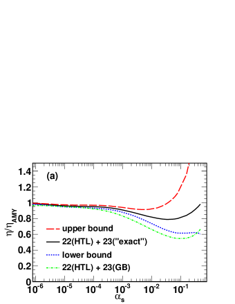
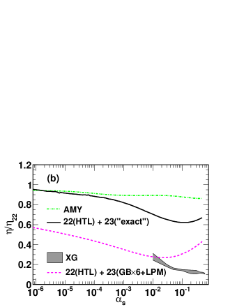
Figure 1: (Color online) (a) The ratio of our numerical result (denoted as “exact”) for the shear viscosity $\eta$ to AMY’s. The error is bounded by the upper and lower bound. The result using the GB matrix element [Eq. (17)] is also shown. (b) Comparison of our result of $\eta/\eta_{22}$ with those of AMY, XG and “GB$\times 6$”(see the text). For our result the HTL gluon propagator is used for the 22 process, the “exact” matrix element Eqs. (5,6,12) are used for the 23 process, and the external gluon mass is set to $m_{\infty}$. In the left panel, the error bands are shown. AMY’s result is taken from Ref. Arnold:2000dr ; Arnold:2003zc and XG’s is from Ref. Wesp:2011yy .

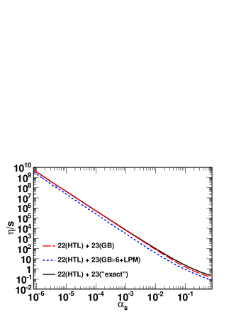
Figure 2: (Color online) $\eta/s$ with various inputs.

In our calculation, we use the HTL propagator for the 22 process. For the 23 process, for technical reasons, we use the internal gluon mass $m_{D}$ instead of the HTL propagator in Eqs. (5-7,12), $E_{p}=\sqrt{\mathbf{p}^{2}+m_{\infty}^{2}}$ in kinematics and $f_{p}^{eq}$ for the external gluon distribution. The errors from not implementing HTL propagator in the 23 process and the modeling of the Landau-Pomeranchuk-Migdal (LPM) effect, and from the uncalculated $O(\sqrt{\alpha_{s}})$ higher order corrections are estimated in Appendix B.

In Fig. 1, we show our main result for the shear viscosity $\eta$ in our previous paper Chen:2009sm , together with the theoretical error band bounded by “upper bound” and “lower bound” curves. Note that previously we estimated the higher order effect to be $O(\alpha_{s})$ suppressed. But since the expansion parameter in finite temperature field theory is $g$ instead of $g^{2}$, we enlarge the error of the higher order effect to $O(\sqrt{\alpha_{s}})$ here. The result agrees with AMY’s result within errors in the left panel although our central value is lower at larger $\alpha_{s}$. If we replace the “exact” matrix element of Eqs. (5-7,12) by the GB matrix element of Eq. (17), then $\eta$ is reduced but still close to the estimated lower bound. This means the 23 collision rate in GB is bigger than that in “exact.”

The effect of the 23 process can be seen more clearly in the ratio $\eta/\eta_{22}$ ($\eta_{22}$ means the shear viscosity with the 22 process included only) shown in the right panel, where we also show AMY’s and XG’s results for comparison. In AMY’s result Arnold:2000dr ; Arnold:2003zc , the near collinear $1\leftrightarrow 2$ process gives $\eta/\eta_{22}$ close to unity. This implies their 12 collision is just a small perturbation to the 22 rate. However, XG employ the soft gluon bremsstrahlung approximation in the matrix element for the 23 process, gives $\eta/\eta_{22}\simeq 0.11\sim 0.16$ around 1/8 in Ref. Xu:2007ns , indicating that their 23 collision rate is about 7 times the 22 one. In their improved treatment using the Kubo relation Wesp:2011yy , they give $\eta/\eta_{22}\simeq 0.1\sim 0.3$, indicating that the 23 collision rate is about 2$\sim$9 times the 22 rate.

Our central result lies between AMY’s and XG’s results. However, even consider the lower bound, our 23 rate does not get bigger than the 22 rate. Thus, it is qualitatively consistent with AMY’s result but inconsistent with XG’s result. When compared with AMY’s result, in addition to the error band shown in the left panel, there is still $\sim 10\%$ difference at $\alpha_{s}=0.01$. This is consistent with the $\sim m_{g}^{2}/T^{2}$ effect from using different inputs for external gluon mass— we use $m_{g}$ while AMY use zero.

We find that we cannot reproduce XG’s result unless we use a 23 matrix element squared at least 6 times larger. To compare with XG’s calculation, we use the same $m_{\infty}=0$ and LPM effect as XG, and

$$\left|M_{12\rightarrow 345}\right|_{CM}^{2}\rightarrow 6\times 54g^{6}N_{g}^{2}\frac{q_{T}^{2}s^{2}}{k_{T}^{2}\left(q_{T}^{2}+m_{D}^{2}\right)^{2}\left[\left(\mathbf{k}_{T}-\mathbf{q}_{T}\right)^{2}+m_{D}^{2}\right]},$$ (52)

which is a slightly different variation of the GB matrix element squared of Eq. (17) multiplied by a factor 6 (denoted as “GB$\times 6$”). This reproduces XG’s result at $\alpha_{s}=0.01$. The origin of this discrepancy is yet to be resolved.

In Fig. 2, $\eta/s$ with various inputs are shown. At $\alpha_{s}=0.3$ and 0.6, the GB$\times 6$ curve yields $\eta/s=0.19$ and 0.09, respectively, while XG has 0.13 and 0.08. The central value of the “exact” result is about two times lager.

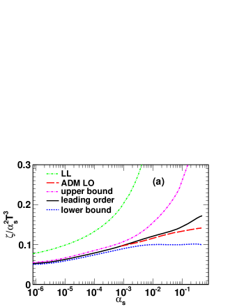
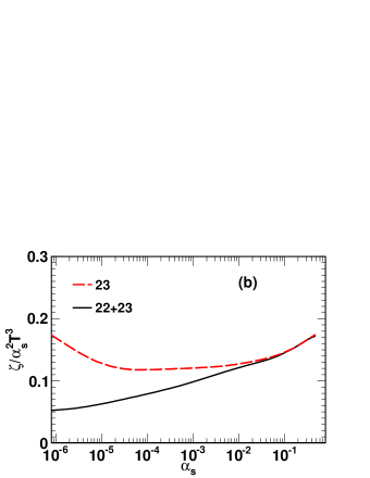
Figure 3: (Color online) (a) Comparison of our result for the bulk viscosity $\zeta$ and its error band (see the appendix) with ADM’s result. ‘LL’ denotes the leading-log result of Eq.(48). ‘ADM LO’ denotes ADM’s leading order result read off from Ref. Arnold:2006fz (only available for $\alpha_{s}\gtrsim 8\times 10^{-4}$). (b) Our full result for $\zeta$ (denoted as 22+23) and $\zeta$ with the 23 process only (denoted as 23).

Our result for the bulk viscosity $\zeta$ using the “exact” matrix element for the 23 process is shown in Fig. 3. We have worked up to $n=6$ and seen good convergence. For example, we obtain $\zeta_{anz}^{(n)}\sim$ 95%, 98%, 99.5% of $\zeta_{anz}^{(6)}$ at $\alpha_{s}=10^{-4}$ for $n=3,4,5$ respectively. The convergence for larger $\alpha_{s}$ is even better. When $\alpha_{s}\lesssim 10^{-8}$, our result approaches the LL one. At larger $\alpha_{s}$, the 23 process becomes more important such that when $\alpha_{s}\gtrsim 0.1$, $\zeta$ is saturated by the 23 contribution (see the right panel of Fig. 3). Our result agrees with that of ADM Arnold:2006fz in the full range of $\alpha_{s}$ within the error band explained in the Appendix B.

IV.4 Angular Correlation in 23 Process

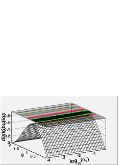
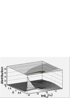
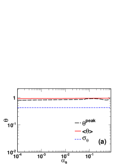
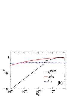
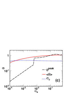
Figure 4: (Color online) The distribution of $\theta$ in the fluid local rest frame. (a) Weighted by the phase space and the Bose-Einstein distribution functions only. (b) Weighted by the contribution to $\eta_{23}$ with the “exact” matrix element. (c) Weighted by the contribution to $\eta_{23}$ with the GB matrix element. The upper panel is normalized to unity for each coupling constant. The lower panel shows the location of the peak $\theta^{peak}$, the average value $<\theta>$ and the variation $\sigma_{\theta}$ of the angle. The angle is in the unit of radian.

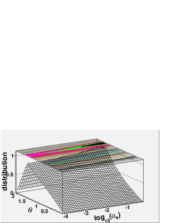
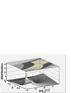
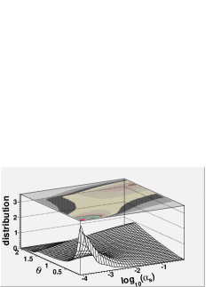
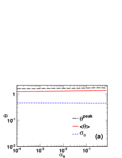
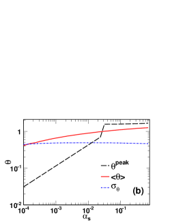
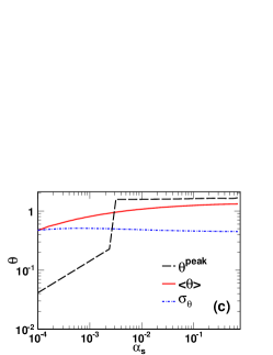
Figure 5: (Color online) Same as Fig. 4 but with $\theta$ in the CM frame.

As mentioned in the introduction, although our result does not provide a model independent check to AMY and ADM’s results, we can still study the angular correlation between final state gluons using our approach. Because the 23 matrix element that we use is exact in vacuum, we can check, modulo some model dependent medium effect, whether the correlation is dominated by the near collinear splittings as asserted by AMY and ADM.

We study the distribution of the minimum angle $\theta$ among the final state gluons. If the near collinear splittings dominate, then the most probable configuration would be that two gluons whose angles are strongly correlated and their relative angle tends to be the smallest among the three relative angles in the final state. This can be seen most easily in the center-of-mass (CM) frame of the 23 collision with two gluons going along about the same direction while the third one is moving in the opposite direction. We expect it is also the case in the fluid local rest frame.

We find that the distribution of $\theta$ is peaked at $\theta^{peak}\sim\sqrt{\alpha_{s}}$, analogous to the near collinear splitting asserted by AMY and ADM. However, the average of $\theta$, $\langle\theta\rangle$, is much bigger than its peak value, as its distribution is skewed with a long tail. Below are more detailed descriptions of our results.

We show the distribution of $\theta$ in the fluid local rest frame in Fig. 4, and show the distribution in the CM frame of the 23 collision in Fig. 5. In both figures, the left panel is the distribution weighted by the phase space and the Bose-Einstein distribution functions, the middle panel is weighted by the 23 contribution to $\eta$ (denoted as $\eta_{23}$, which is the $\eta$ analogy of the second term in Eq. (29)) with the “exact” matrix element, and the right panel is similar to the middle one with the GB matrix element.

We first look at the distribution in the fluid local rest frame in Fig. 4. The left panel plots do not depend on the interaction and hence is $\alpha_{s}$ independent. The distribution has $\theta^{peak}\simeq\left\langle\theta\right\rangle$ and the variation $\sigma_{\theta}$ is about the same size. In the middle panel, the $\eta_{23}$ weighted distribution with the “exact” matrix element, on the other hand, has $\theta^{peak}\sim\sqrt{\alpha_{s}}$ at small $\alpha_{s}$, while $\left\langle\theta\right\rangle$ is significantly bigger and $\sigma_{\theta}$ is close to its value in the left panel. In the right panel, where the GB matrix element is used, $\theta^{peak}$ is still close to be proportional to$\sqrt{\alpha_{s}}$ at small $\alpha_{s}$, but the angle is about twice as big as the “exact” case.

The distribution in the 23 collision CM frame shown in Fig. 5 has a similar behavior as that in the fluid local rest frame but the angles are in general much larger.

The above analysis suggests that the GB formula, which takes the soft gluon bremsstrahlung limit in the CM frame, still has some near collinear splitting behavior in the fluid local rest frame. It is curious what the nature of the long tail is. We will leave it for future investigation.

IV.5 More aspects

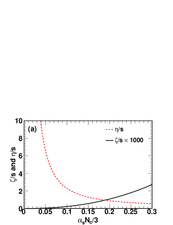
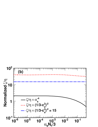
Figure 6: (Color online) Universal curves for $\zeta/s$ (this work), $\eta/s$ Chen:2010xk and their ratio. These curves are universal and suitable for a general $SU(N_{c})$ pure gauge theory.

In Fig. 6, our results for $\zeta/s$ and $\eta/s$ ($\eta/s$ is computed in Ref. Chen:2010xk ) using the “exact” matrix element for the 23 process are shown in the left panel and their ratio $\zeta/\eta$ in units of $\alpha_{s}^{4}$ and $\left(1/3-c_{s}^{2}\right)^{2}$ in the right panel. As we emphasize in Sec. IV.1, these are universal curves suitable for a general $SU(N_{c})$ pure gauge theory.

The external gluon mass $m_{\infty}$ is included in the entropy density $s$ here, but it is a higher order effect and numerically very small at small $\alpha_{s}$. In the range where perturbation theory is reliable ($\alpha_{s}\lesssim 0.1$), $\zeta$ is always smaller than $\eta$ by at least three orders of magnitude. One can see that our result of $\zeta/\eta$ agrees with $15\left(1/3-c_{s}^{2}\right)^{2}$ of Weinberg parametrically Weinberg:1971mx , and it is rather close to the LL one in Eq. (50).

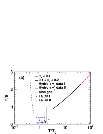
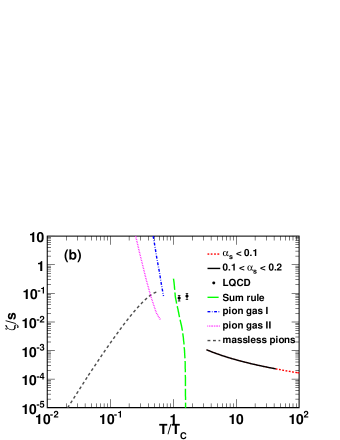
Figure 7: (Color online) (a) $\eta/s$ for a pion gas Chen:2006iga and a gluon plasma with LQCD Meyer:2007ic ; Meyer:2009jp ; Nakamura:2004sy and perturbative QCD Chen:2010xk , together with $\eta/s$ extracted from RHIC elliptical flow ($v_{2}$): I Luzum:2008cw and II Song:2008hj . The arrow below the line of "Hydro+$v_{2}$ data II" indicates that it is an upper bound. (b) $\zeta/s$ for a massive Lu:2011df ; FernandezFraile:2008vu and massless Chen:2006iga pion gas and a gluon plasma with LQCD Meyer:2010ii and perturbative QCD (this work). The sum rule result Karsch:2007jc is for $N_{f}=3$. The massive pion curves are denoted as "pion gas I" (inelastic process Lu:2011df ) and "pion gas II" (elastic process FernandezFraile:2008vu ).

In Fig. 7, we have plotted $\eta/s$ vs. $T/T_{c}$ and $\zeta/s$ vs. $T/T_{c}$ for QCD with various number of light quark flavors $N_{f}$ (and different $T_{c}$’s are used in different systems) at zero baryon chemical potential. In $\eta/s$, $T/T_{c}\ll 1$, the QCD result is calculated by the pion gas system using the Boltzmann equation Chen:2006iga (the kaon mass is more than two time bigger than $T_{c}$ —too heavy to be important for $T/T_{c}\ll 1$; for other calculations in hadronic gases, see Prakash:1993bt ; Dobado:2003wr ; Dobado:2001jf ; Chen:2007xe ; Itakura:2007mx ). The $T/T_{c}\gtrsim 1$ result is for gluon plasma using lattice QCD (LQCD) Meyer:2007ic ; Meyer:2009jp ; Nakamura:2004sy (see Meyer:2011gj for a recent review; for a lattice inspired model around $T_{c}$, see e.g. Ref. Hidaka:2009ma ). This result has assumed a certain functional form for the spectral function and hence has some model dependence. Note that in this temperature region, there might be anomalous shear viscosity arising from coherent color fields in the early stage of the QGP Asakawa:2006tc . We have also shown the value of $\eta/s$ extracted from the elliptic flow ($v_{2}$) data of RHIC using hydrodynamics: $\eta/s=0.1\pm 0.1(\mathrm{theory})\pm 0.08(\mathrm{experiment})$ Luzum:2008cw (denoted as “Hydro$+v_{2}$ data I”) and $\eta/s<5\times 1/(4\pi)$ Song:2008hj (denoted as “Hydro$+v_{2}$ data II”). And we have assigned a conservative temperature range $T=0.24\pm 0.10$ GeV that covers the initial and final temperatures in the hydrodynamic evolution ($T_{f}=0.14$ GeV, $T_{i}\lesssim 0.34$ GeV).

For $T/T_{c}\gg 1$, we use the perturbative result of the gluon plasma with the 22 and 23 processes in the Boltzmann equation Chen:2010xk and the standard two-loop renormalization (the scheme dependence is of higher order) for the SU(3) pure gauge theory

$$\frac{1}{4\pi\alpha_{s}\left(T\right)}=2\beta_{0}\ln\left(\frac{\mu T}{\Lambda_{\overline{MS}}}\right)+\frac{\beta_{1}}{\beta_{0}}\ln\left(2\ln\left(\frac{\mu T}{\Lambda_{\overline{MS}}}\right)\right),$$ (53)

where $\beta_{0}=11/(16\pi^{2})$ and $\beta_{1}=102/(16\pi^{2})^{2}$. Fitting to lattice data at $1.2\lesssim T/T_{c}\lesssim 2$ yields $\mu\simeq 1.14\pi$, $\Lambda_{\overline{MS}}\simeq 261$ MeV and $T_{c}\simeq 202$ MeV Kaczmarek:2005ui . When $T/T_{c}\simeq 3.3$ and $42$, $\alpha_{s}=0.2$ and $0.1$, respectively. If $\eta/s$ above $T_{c}$ is dominated by the gluon contribution so the gluon plasma result ($N_{f}=0$) is close to that of $N_{f}=3$ QCD , then Fig. 7 shows that $\eta/s$ might have a local minimum at $T_{c}$ Csernai:2006zz ; Chen:2006iga ; Bluhm:2010qf .

For $\zeta/s$ with $T/T_{c}\ll 1$, the QCD result is calculated by the Boltzmann equation for massless Chen:2007kx  and massive Lu:2011df ; FernandezFraile:2008vu (also in Ref. Dobado:2011qu ; Chakraborty:2010fr ) pions. For massless pions, $\zeta/s$ is increasing in $T$ since it is expected when the pion self-coupling vanishes (or equivalently the pion decay constant $f_{\pi}\rightarrow\infty$), $\zeta$ also vanishes. Thus, the dimensionless combination $\zeta/s\propto\left(T/f_{\pi}\right)^{z}$, where $z$ is some positive number. For massive pions, the expected non-relativistic limit for the bulk viscosity reads FernandezFraile:2008vu $\zeta\sim f^{4}_{\pi}\sqrt{T}/m_{\pi}^{3/2}$, where $m_{\pi}=$138 MeV is the physical pion mass and one uses Weinberg’s low-energy result for the pion-pion cross section at low energy (low temperature) [72]. This suggests the (non-relativistic) conformal symmetry is recovered at zero $T$ when particle number conservation is imposed. In the relativistic case, Ref. Lu:2011df argues that the number changing process (the 24 process, 23 not allowed by parity conservation) is slower than 22, so it controls the time scale for the system to go back to thermal equilibrium. At low enough $T$, this time scale is very long since there are not many pions energetic enough to collide and produce four pions. However, if the time scale is longer than that of the fire ball expansion at RHIC, the elastic scattering FernandezFraile:2008vu ; Prakash:1993bt ; Davesne:1995ms (see also NoronhaHostler:2008ju ; Paech:2006st ) is more relevant phenomenologically. For $T/T_{c}\gtrsim 1$, lattice QCD calculation of a gluon plasma is shown Meyer:2010ii together with the sum rule result with $N_{f}=3$ Kharzeev:2007wb ; Karsch:2007jc . Both of them have some model dependence on the shape of the spectral function used. This issue was discussed extensively in Refs. Teaney:2006nc ; Moore:2008ws ; Romatschke:2009ng which inspired Ref. Meyer:2010ii to include a delta function contribution to the spectral function which was missed in the earlier result of Ref. Meyer:2007dy . The same delta function will modify the sum rule result Kharzeev:2007wb ; Karsch:2007jc as well. This is yet to be worked out.

For $T/T_{c}\gg 1$, the perturbative result of the gluon plasma calculated in this work is shown. We see that although $\zeta/s$ for the massive pion case is decreasing in $T$ for small $T$. It should merge to the massless pion result when the pion thermal energy $\sim 3T$ is bigger than $m_{\pi}$. Thus, it is still possible that $\zeta/s$ has a local maximum at $T_{c}$ as in some model calculations Gubser:2008yx ; Li:2009by ; Bluhm:2010qf provided there is no much difference between the $N_{f}=0$ and $N_{f}=3$ results above $T_{c}$.

It is very interesting that $\zeta>\eta$ for the gluon plasma just above $T_{c}$. This suggests a fluid could still be perfect without being conformal, like the AdS/CFT model of Ref. Gubser:2008yx . Finally, it is intriguing that $\eta/s$ might have a local minimum at $T_{c}$ and $\zeta/s$ might have a local maximum at $T_{c}$. However, despite there are many other systems exhibiting this behavior for $\eta/s$ Csernai:2006zz ; Lacey:2006bc ; Chen:2007xe ; Chen:2007jq , there are counterexamples showing that it is not universal Chen:2010vf ; Chen:2010vg ; Dobado:2009ek ; FernandezFraile:2010gu .

V Conclusions

We have calculated the shear and bulk viscosity of a weakly interacting gluon plasma with 22 and 23 collisional processes and a simple treatment to model the LPM effect. Our results agree with the results of AMY and ADM within errors. By studying the 23 contribution to $\eta$, we find that the minimum angle $\theta$ among the final state gluons has a distribution that is peaked at $\theta\sim\sqrt{\alpha_{s}}$, analogous to the near collinear splitting asserted by AMY and ADM. However, the average of $\theta$ is much bigger than its peak value, as its distribution is skewed with a long tail which is worth further exploration. The same $\theta$ behavior is also seen if the 23 matrix element is taken to the soft gluon bremsstrahlung limit in the CM frame. This suggests that the soft gluon bremsstrahlung in the CM frame still has some near collinear behavior in the fluid local rest frame. We also generalize our result to a general $SU(N_{c})$ pure gauge theory and summarize the current theoretical results for viscosities in QCD.

Acknowledgement: QW thanks C. Greiner for bringing our attention to their latest results about the shear viscosity for the 23 process. We thank G. Moore for useful communications related to his work. JWC thanks INT, Seattle, for hospitality. JWC is supported by the NSC, NCTS, and CASTS of ROC. QW is supported in part by the National Natural Science Foundation of China (NSFC) under grant 10735040 and 11125524. HD is supported in part by the NSFC under grant 11105084 and the Natural Science Foundation of the Shandong province under grant ZR2010AQ008. JD is supported in part by the NSFC under grant 11105082 and the Innovation Foundation of Shandong University under grant 2010GN031.

Appendix A Soft gluon bremsstrahlung

In this appendix, we give the details of the derivation of the GB formula or the matrix element for the soft gluon bremsstrahlung. We work in the CM frame of the initial or final state where the longitudinal direction is defined as that of $\mathbf{p}_{1}$ or $\mathbf{p}_{2}$. The conditions for the soft gluon bremsstrahlung are: $s\gg p_{iT}$ and $k_{T}\gg yq_{T}$ (or $s\rightarrow\infty$ and $y\rightarrow 0$). This means the energy of the bremsstrahlung gluon, say $E_{5}$, is much smaller than other two gluons, $E_{5}\ll E_{3},E_{4}$.

It is convenient to use the Mandelstam-like variables defined as

$$s=(p_{1}+p_{2})^{2},\;t=(p_{1}-p_{3})^{2},\;u=(p_{1}-p_{4})^{2},$$

$$s^{\prime}=(p_{3}+p_{4})^{2},\;t^{\prime}=(p_{2}-p_{4})^{2},\;u^{\prime}=(p_{2}-p_{3})^{2},$$

$$T_{i5}=(k_{i}+k_{5})^{2},\;\;(i=1,2,3,4).$$ (54)

Here we assume all gluons are massless, so we obtain

$$(12)=\frac{s}{2},\;(13)=-\frac{t}{2},\;(14)=-\frac{u}{2},$$

$$(23)=-\frac{u^{\prime}}{2},\;(24)=-\frac{t^{\prime}}{2},\;(34)=\frac{s^{\prime}}{2},$$

$$(15)=\frac{T_{15}}{2},\;(25)=\frac{T_{25}}{2},\;(35)=\frac{T_{35}}{2},\;(45)=\frac{T_{45}}{2}.$$ (55)

Using light-cone variables in Eq. (13) and taking the limit $s\rightarrow\infty$ or $s\gg p_{iT}^{2}$, we have

$$t = -\frac{1}{1-y}(\mathbf{q}_{T}-\mathbf{k}_{T})^{2},$$

$$u \approx -s,$$

$$s^{\prime} \approx (1-y)s,$$

$$t^{\prime} = -q_{T}^{2},$$

$$u^{\prime} = -(1-y)s,$$

$$T_{15} \approx k_{T}^{2}/y,$$

$$T_{25} \approx ys,$$

$$T_{35} \approx \frac{(\mathbf{k}_{T}-y\mathbf{q}_{T})^{2}}{(1-y)y},$$

$$T_{45} \approx ys.$$ (56)

We see that $t,t^{\prime},T_{i5}(i=1,2,3,4)$ are small. In evaluating $\left|M_{12\rightarrow 345}\right|^{2}$, we denote $(12345)\equiv 1/[\left(12\right)\left(23\right)\left(34\right)\left(45\right)\left(51\right)]$, and we can evaluate all quantities in the denominator of Eq. (5),

$$(12345) = -\frac{1}{su^{\prime}s^{\prime}T_{15}T_{45}},$$

$$(12354) = \frac{1}{su^{\prime}uT_{35}T_{45}},$$

$$(12435) = -\frac{2^{5}}{ss^{\prime}t^{\prime}T_{15}T_{35}},$$

$$(12453) = \frac{1}{stt^{\prime}T_{35}T_{45}},$$

$$(12534) = -\frac{1}{ss^{\prime}uT_{25}T_{35}},$$

$$(12543) = -\frac{1}{ss^{\prime}tT_{25}T_{45}},$$

$$(13245) = -\frac{1}{u^{\prime}tt^{\prime}T_{15}T_{45}},$$

$$(13254) = -\frac{1}{uu^{\prime}tT_{25}T_{45}},$$

$$(13425) = \frac{1}{s^{\prime}tt^{\prime}T_{15}T_{25}},$$

$$(13524) = -\frac{1}{utt^{\prime}T_{25}T_{35}},$$

$$(14235) = -\frac{1}{uu^{\prime}t^{\prime}T_{15}T_{35}},$$

$$(14325) = \frac{1}{uu^{\prime}s^{\prime}T_{15}T_{25}},$$ (57)

where we have factored out $2^{5}$. Note that other permutations which do not appear are given by the identity $(12345)=(15432)$. Then we can collect the most singular parts involving $t,t^{\prime},T_{i5}(i=1,2,3,4)$ in the denominator and obtain

$$\left|M_{12\rightarrow 345}\right|^{2} \sim \frac{1}{stt^{\prime}T_{35}T_{45}}-\frac{1}{u^{\prime}tt^{\prime}T_{15}T_{45}}+\frac{1}{s^{\prime}tt^{\prime}T_{15}T_{25}}-\frac{1}{utt^{\prime}T_{25}T_{35}},$$ (58)

$$-\frac{1}{ss^{\prime}t^{\prime}T_{15}T_{35}}-\frac{1}{ss^{\prime}tT_{25}T_{45}}-\frac{1}{uu^{\prime}tT_{25}T_{45}}-\frac{1}{uu^{\prime}t^{\prime}T_{15}T_{35}},$$

$$\sim \frac{2}{s^{2}q_{T}^{2}}\left[\frac{1}{(\mathbf{q}_{T}-\mathbf{k}_{T})^{2}}\frac{(1-y)^{2}}{(\mathbf{k}_{T}-y\mathbf{q}_{T})^{2}}+\frac{1}{(\mathbf{q}_{T}-\mathbf{k}_{T})^{2}}\frac{1}{k_{T}^{2}}+\frac{y^{2}}{(\mathbf{k}_{T}-y\mathbf{q}_{T})^{2}k_{T}^{2}}\right].$$

One can see that the matrix element squared has singularities from three poles at $k_{T}^{2}=0$, $(\mathbf{q}_{T}-\mathbf{k}_{T})^{2}=0$. For the soft limit, $k_{T}\gg yq_{T}$, this can be realized by setting $y\rightarrow 0$, we obtain

$$\left|M_{12\rightarrow 345}\right|_{soft}^{2}\sim\frac{4}{s^{2}q_{T}^{2}}\frac{1}{(\mathbf{q}_{T}-\mathbf{k}_{T})^{2}k_{T}^{2}},$$ (59)

which reproduces the GB formula.

Appendix B Error Estimation

The error bands of $\eta$ and $\zeta$ shown in Figs. 1 and 3 are based on the estimation of the following errors:

(a) HTL corrections for the 23 process: In the 22 process, if we replace the HTL scattering amplitude of Eq. (7) by that of Eq. (9) with $m_{D}$ as the regulator, then the 22 collision rate is reduced by $\sim 30\%$ for $\alpha_{s}\simeq 0.005$-$0.1$. At smaller $\alpha_{s}$, the effect becomes smaller and eventually becomes negligible at $\alpha_{s}=10^{-8}$. The reduction arises because the HTL magnetic screening effect gives a smaller IR cut-off than $m_{D}$. Analogously, using $m_{D}$ as the regulator in the 23 process tends to under-estimate the 23 collision rate and gives a larger $\eta$ and $\zeta$.

(b) LPM effect: Our previous calculation on $\eta$ using the Gunion-Bertsch formula shows that implementing the $m_{D}$ regulator gives a very close result to the LPM effect Chen:2009sm . Thus, we will estimate the size of the LPM effect by increasing the external gluon mass $m_{g}$ from $m_{\infty}$ to $m_{D}$.

(c) Higher order effect: The higher order effect is parametrically suppressed by $O(\sqrt{\alpha_{s}})$, but the size is unknown. Computing this effect requires a treatment beyond the Boltzmann equation Hidaka:2010gh and the inclusion of the 33 and 24 processes. We just estimate the effect to be $\sqrt{\alpha_{s}}$ times the leading order which is $\sim 10\%$ at $\alpha_{s}=0.01$. (Note that we estimated the higher order effect to be $O(\alpha_{s})$ suppressed in Ref. Chen:2009sm . But since the expansion parameter in finite temperature field theory is $g$ instead of $g^{2}$, we enlarge the error here.)

Combining the above analyses, we consider errors from (a) to (c). To compute a recommended range of $\zeta$ (the range of $\eta$ is computed analogously), we will work with the $R_{22}$ and $R_{23}$ collision rates defined as

$$R_{23}^{-1} \equiv \zeta_{23},$$

$$\left(R_{22}+R_{23}\right)^{-1} \equiv \zeta_{22+23},$$ (60)

where $\zeta_{23}$ is the bulk viscosity for a collision with the 23 process only. Using HTL instead of $m_{D}$ for the gluon propagator enhances the 22 rate by a factor of

$$\delta\equiv\frac{R_{22(HTL)}}{R_{22(MD)}}.$$ (61)

We will assume that the same enhancement factor appears in 23 rate as well, such that

$$\frac{R_{23(HTL)}}{R_{23(MD)}}\simeq\delta.$$ (62)

On the other hand, the LPM effect is estimated to suppress the 23 rate by a factor of

$$\gamma=\frac{R_{23(LPM)}}{R_{23(MD)}}.$$ (63)

Combining the estimated HTL and LPM corrections to the 23 rate, the 22+23 rate is likely to be in the range $[R_{22}+R_{23},R_{22}+\gamma\delta R_{23}]$, while the higher order effect gives $\pm\sqrt{\alpha_{s}}\left(R_{22}+R_{23}\right)$ corrections to the rate. Without further information, the errors are assumed to be Gaussian and uncorrelated, the total rate is

$$\left(R_{22}+\frac{\gamma\delta+1}{2}R_{23}\right)\pm\left(\frac{\gamma\delta-1}{2}R_{23}\right)\pm\sqrt{\alpha_{s}}\left(R_{22}+R_{23}\right),$$ (64)

and the recommended upper ($\zeta_{+}$) and lower ($\zeta_{-}$) range for $\zeta$ are

$$\zeta_{\pm}=\frac{1}{\left(R_{22}+\frac{\gamma\delta+1}{2}R_{23}\right)\mp\sqrt{\left(\frac{\gamma\delta-1}{2}R_{23}\right)^{2}+\alpha_{s}\left(R_{22}+R_{23}\right)^{2}}}.$$ (65)

The $\zeta_{\pm}$ values are shown in the left panel of Fig. 3.

References

- (1) P. Arnold, G. D. Moore and L. G. Yaffe, JHEP 0011, 001 (2000).
- (2) P. B. Arnold, C. Dogan and G. D. Moore, Phys. Rev. D 74, 085021 (2006).
- (3) P. Kovtun, D. T. Son and A. O. Starinets, Phys. Rev. Lett. 94, 111601 (2005).
- (4) A. Buchel, J.T. Liu, Phys. Rev. Lett. 93, 090602 (2004).
- (5) A. Buchel, Phys. Lett. B, 609:392 (2005).
- (6) J. M. Maldacena, Adv. Theor. Math. Phys. 2, 231 (1998) [Int. J. Theor. Phys. 38, 1113 (1999)].
- (7) S. S. Gubser, I. R. Klebanov and A. M. Polyakov, Phys. Lett. B 428, 105 (1998)
- (8) E. Witten, Adv. Theor. Math. Phys. 2, 253 (1998)
- (9) I. Arsene et al. [BRAHMS Collaboration], Nucl. Phys. A 757, 1 (2005).
- (10) B. B. Back et al., Nucl. Phys. A 757, 28 (2005).
- (11) K. Adcox et al. [PHENIX Collaboration], Nucl. Phys. A 757, 184 (2005).
- (12) M. Luzum and P. Romatschke, Phys. Rev. C 78, 034915 (2008).
- (13) H. Song and U. W. Heinz, J. Phys. G 36, 064033 (2009).
- (14) H. B. Meyer, Phys. Rev. D 76, 101701 (2007).
- (15) D. Kharzeev, K. Tuchin, JHEP 0809, 093 (2008).
- (16) F. Karsch, D. Kharzeev, K. Tuchin, Phys. Lett. B663, 217-221 (2008).
- (17) P. Arnold, G. D. Moore and L. G. Yaffe, JHEP 0305, 051 (2003).
- (18) Z. Xu and C. Greiner, Phys. Rev. Lett. 100, 172301 (2008).
- (19) C. Wesp, A. El, F. Reining, Z. Xu, I. Bouras and C. Greiner, Phys. Rev. C 84, 054911 (2011).
- (20) J. W. Chen, J. Deng, H. Dong and Q. Wang, Phys. Rev. D 83, 034031 (2011).
- (21) S. Jeon, Phys. Rev. D 52, 3591 (1995).
- (22) S. Jeon and L. G. Yaffe, Phys. Rev. D 53, 5799 (1996).
- (23) M. E. Carrington, D. f. Hou and R. Kobes, Phys. Rev. D 62, 025010 (2000).
- (24) E. Wang and U. W. Heinz, Phys. Lett. B 471, 208 (1999).
- (25) Y. Hidaka and T. Kunihiro, Phys. Rev. D 83, 076004 (2011).
- (26) J. S. Gagnon and S. Jeon, Phys. Rev. D 76, 105019 (2007).
- (27) U. W. Heinz, Annals Phys. 161, 48 (1985).
- (28) H. T. Elze, M. Gyulassy and D. Vasak, Nucl. Phys. B 276, 706 (1986).
- (29) T. S. Biro, E. van Doorn, B. Muller, M. H. Thoma and X. N. Wang, Phys. Rev. C 48, 1275 (1993).
- (30) J. P. Blaizot and E. Iancu, Nucl. Phys. B 557, 183 (1999).
- (31) R. Baier, A. H. Mueller, D. Schiff and D. T. Son, Phys. Lett. B 502, 51 (2001).
- (32) Q. Wang, K. Redlich, H. Stoecker and W. Greiner, Phys. Rev. Lett. 88, 132303 (2002).
- (33) F. A. Berends, R. Kleiss, P. De Causmaecker, R. Gastmans and T. T. Wu, Phys. Lett. B 103, 124 (1981).
- (34) R. K. Ellis and J. C. Sexton, Nucl. Phys. B 269, 445 (1986).
- (35) T. Gottschalk and D. W. Sivers, Phys. Rev. D 21, 102 (1980).
- (36) H. A. Weldon, Phys. Rev. D 26, 1394 (1982).
- (37) R. D. Pisarski, Phys. Rev. Lett. 63, 1129 (1989).
- (38) H. Heiselberg and X. N. Wang, Nucl. Phys. B 462, 389 (1996).
- (39) J. P. Blaizot, E. Iancu and A. Rebhan, Phys. Rev. D 63, 065003 (2001).
- (40) J. O. Andersen, E. Braaten, E. Petitgirard and M. Strickland, Phys. Rev. D 66, 085016 (2002).
- (41) S. Caron-Huot and G. D. Moore, Phys. Rev. Lett. 100, 052301 (2008).
- (42) J. W. Chen, H. Dong, K. Ohnishi and Q. Wang, Phys. Lett. B 685, 277 (2010).
- (43) J. F. Gunion and G. Bertsch, Phys. Rev. D 25, 746 (1982).
- (44) S. K. Das and J. e. Alam, Phys. Rev. D 82, 051502 (2010).
- (45) S. KDas and J. -eAlam, Phys. Rev. D 83, 114011 (2011).
- (46) R. Abir, C. Greiner, M. Martinez and M. G. Mustafa, Phys. Rev. D 83, 011501 (2011).
- (47) T. Bhattacharyya, S. Mazumder, S. K. Das and J. e. Alam, Phys. Rev. D 85, 034033 (2012).
- (48) M. Gyulassy, M. Plumer, M. Thoma and X. N. Wang, Nucl. Phys. A 538, 37C (1992).
- (49) X. -N. Wang, M. Gyulassy and M. Plumer, Phys. Rev. D 51, 3436 (1995).
- (50) P. Résibois and M. d. Leener, Classical Kinetic Theory of Fluids (John Wiley Sons, 1977).
- (51) G. Baym, H. Monien, C. J. Pethick and D. G. Ravenhall, Phys. Rev. Lett. 64, 1867 (1990).
- (52) H. Heiselberg, Phys. Rev. D 49, 4739 (1994).
- (53) S. Weinberg, Astrophys. J. 168, 175 (1971).
- (54) J. W. Chen and E. Nakano, Phys. Lett. B 647, 371 (2007).
- (55) M. Prakash, M. Prakash, R. Venugopalan and G. Welke, Phys. Rept. 227, 321 (1993).
- (56) A. Dobado and F. J. Llanes-Estrada, Phys. Rev. D 69, 116004 (2004).
- (57) A. Dobado and S. N. Santalla, Phys. Rev. D 65, 096011 (2002).
- (58) J. W. Chen, Y. H. Li, Y. F. Liu and E. Nakano, Phys. Rev. D 76, 114011 (2007).
- (59) K. Itakura, O. Morimatsu and H. Otomo, Phys. Rev. D 77, 014014 (2008).
- (60) H. B. Meyer, Nucl. Phys. A 830, 641C (2009).
- (61) A. Nakamura and S. Sakai, Phys. Rev. Lett. 94, 072305 (2005).
- (62) H. B. Meyer, Eur. Phys. J. A 47, 86 (2011).
- (63) Y. Hidaka and R. D. Pisarski, Phys. Rev. D 81, 076002 (2010).
- (64) M. Asakawa, S. A. Bass and B. Muller, Phys. Rev. Lett. 96, 252301 (2006).
- (65) O. Kaczmarek and F. Zantow, Phys. Rev. D 71, 114510 (2005).
- (66) L. P. Csernai, J. I. Kapusta and L. D. McLerran, Phys. Rev. Lett. 97, 152303 (2006).
- (67) M. Bluhm, B. Kampfer and K. Redlich, Phys. Rev. C 84, 025201 (2011).
- (68) J. -W. Chen, J. Wang, Phys. Rev. C79, 044913 (2009).
- (69) E. Lu, G. D. Moore, Phys. Rev. C83, 044901 (2011).
- (70) D. Fernandez-Fraile and A. Gomez Nicola, Phys. Rev. Lett. 102, 121601 (2009).
- (71) A. Dobado, F. J. Llanes-Estrada and J. M. Torres-Rincon, Phys. Lett. B 702, 43 (2011).
- (72) P. Chakraborty and J. I. Kapusta, Phys. Rev. C 83, 014906 (2011).
- (73) D. Davesne, Phys. Rev. C 53, 3069 (1996).
- (74) J. Noronha-Hostler, J. Noronha and C. Greiner, Phys. Rev. Lett. 103, 172302 (2009).
- (75) K. Paech and S. Pratt, Phys. Rev. C 74, 014901 (2006).
- (76) H. B. Meyer, JHEP 1004, 099 (2010).
- (77) D. Teaney, Phys. Rev. D74, 045025 (2006).
- (78) G. D. Moore, O. Saremi, JHEP 0809, 015 (2008).
- (79) P. Romatschke, D. T. Son, Phys. Rev. D80, 065021 (2009).
- (80) H. B. Meyer, Phys. Rev. Lett. 100, 162001 (2008).
- (81) S. S. Gubser, A. Nellore, S. S. Pufu and F. D. Rocha, Phys. Rev. Lett. 101, 131601 (2008).
- (82) B. C. Li and M. Huang, Phys. Rev. D 80, 034023 (2009).
- (83) R. A. Lacey et al., Phys. Rev. Lett. 98, 092301 (2007).
- (84) J. -W. Chen, M. Huang, Y. -H. Li, E. Nakano and D. -L. Yang, Phys. Lett. B 670, 18 (2008).
- (85) J. -W. Chen, C. -T. Hsieh and H. -H. Lin, Phys. Lett. B 701, 327 (2011).
- (86) J. -W. Chen, M. Huang, C. -T. Hsieh and H. -H. Lin, Phys. Rev. D 83, 115006 (2011).
- (87) A. Dobado, F. J. Llanes-Estrada and J. M. Torres-Rincon, Phys. Rev. D 80, 114015 (2009).
- (88) D. Fernandez-Fraile, Phys. Rev. D 83, 065001 (2011).