Resonances for “large” ergodic systems in one dimension: a review

Abstract.

The present note reviews recent results on resonances for one-dimensional quantum ergodic systems constrained to a large box. We restrict ourselves to one dimensional models in the discrete case. We consider two type of ergodic potentials on the half-axis, periodic potentials and random potentials. For both models, we describe the behavior of the resonances near the real axis for a large typical sample of the potential. In both cases, the linear density of their real parts is given by the density of states of the full ergodic system. While in the periodic case, the resonances distribute on a nice analytic curve (once their imaginary parts are suitably renormalized), in the random case, the resonances (again after suitable renormalization of both the real and imaginary parts) form a two dimensional Poisson cloud.

0. Introduction

On $\ell^{2}(\mathbb{N})$, consider $V$ a bounded potential and the operator $H=-\Delta+V$ satisfying the Dirichlet boundary condition at $0$.
The potentials $V$ we will consider with are of two types:

• $V$ periodic;

• $V=V_{\omega}$ random e.g. a collection of i.i.d. random variables.

The spectral theory of such models has been studied extensively (see e.g. [10]) and it is well known that, when considered on $\ell^{2}(\mathbb{Z})$, the spectrum of $H$ is purely absolutely continuous when $V$ is periodic ([24]) while it is pure point when $V=V_{\omega}$ is the Anderson potential ([2, 20]). On $\ell^{2}(\mathbb{N})$, the picture is the same except for possible discrete eigenvalues outside the essential spectrum which coincides and is of the same nature as the essential spectrum of the operator on $\ell^{2}(\mathbb{Z})$.
Let $L>0$. The object of our study is the following operator on $\ell^{2}(\mathbb{N})$

(0.1) $$H_{L}=-\Delta+V\mathbf{1}_{\llbracket 0,L\rrbracket}$$

when $L$ becomes large; here $-\Delta$ is the free Lapalce operator defined by $-(\Delta u)(n)=u(n+1)+u(n-1)$ for $n\geq 0$ where $u=(u(n))_{n\geq 0}\in\ell^{2}(\mathbb{N})$ and $u(-1)=0$ (Dirichlet boundary condition at $0$).
Clearly, the essential spectrum of $H_{L}$ is that of the discrete Laplace operator, that is, $[-2,2]$, and it is absolutely continuous. Moreover, outside this absolutely continuous spectrum, $H_{L}$ has only discrete eigenvalues associated to exponentially decaying eigenfunctions.
We are interested in the resonances of the operator $H_{L}$. These can be defined as the poles of the meromorphic continuation of the resolvent of $H_{L}$ through the continuous spectrum of $H_{L}$ (see e.g. [25]). One proves that

Theorem 1.

The operator valued holomorphic function $z\in\mathbb{C}^{+}\mapsto(z-H_{L})^{-1}$ admits a meromorphic continuation from $\mathbb{C}^{+}$ to $\displaystyle\mathbb{C}\setminus\left((-\infty,2]\cup[2,+\infty)\right)$ (see Fig. 1) with values in the operators from $\ell^{2}_{\text{comp}}(\mathbb{N})$ to $\ell^{2}_{\text{loc}}(\mathbb{N})$.
Moreover, the number of poles of this meromorphic continuation in the lower half-plane is equal to $L+1$.

As said, we define the resonances as the poles of this meromorphic continuation. The resonance widths, the imaginary part of the resonances, play an important role in the large time behavior of $\displaystyle e^{-itH_{L}}$, especially the smallest width that gives the leading order contribution (see [25, 26, 17]).

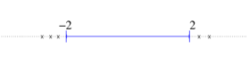
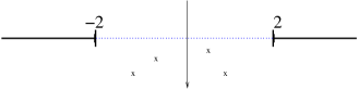
Figure 1. The spectrum of $H_{L}$ and the analytic continuation of $(z-H_{L})^{-1}$

As $L\to+\infty$, $H_{L}$ converges to $H$ in the strong resolvent sense. Thus, it is natural to expect that the differences in the spectral nature between the cases $V$ periodic and $V$ random should reflect into differences in the behavior of the resonances. As we shall see, this is the case.
Our goal is to describe the resonances or, rather, their statistical properties and relate them (the distribution of the resonances, the distribution of the widths) to the spectral characteristics of $H=-\Delta+V$. In the periodic case, we expect that the Bloch-Floquet data for the operator $-\Delta+V$ on $\ell(\mathbb{Z})$ will be of importance; in the random case, this role should be taken over by the distribution of the eigenvalues of $-\Delta+V_{\omega}$.The scattering theory or the closely related study of resonances for the operator (0.1) or for similar one-dimensional models has already been discussed in various works both in the mathematical and physical literature [6, 5, 14, 22, 3, 15, 1, 13, 23, 16]. The proofs of the result we present below will be released elsewhere ([12]). Though we will restrict ourselves to the discrete model, the continuous model can be dealt with in a very similar way.Let us now describe our results. We start with the periodic case and turn to the random case in the next section.

1. The periodic case

We assume that, for some $p>0$, one has

(1.1) $$V_{n+p}=V_{n}\quad\text{for all}\quad n\geq 0.$$

Let $\Sigma^{\prime}$ be the spectrum of $H$ acting on $\ell^{2}(\mathbb{N})$ and $\Sigma_{0}$ be the spectrum of $-\Delta+V$ acting on $\ell^{2}(\mathbb{Z})$. One then has the following description for the spectra:

• $\displaystyle\Sigma^{\prime}=\Sigma_{0}=\bigcup_{j=1}^{p}[a_{j}^{-},a_{j}^{+}]$ for some $a_{j}^{-}<a_{j}^{+}$ ($p\geq 1$) and the spectrum is purely absolutely continuous (see e.g. [24]); the spectral resolution can be obtained via a Bloch-Floquet decomposition;

• on $\ell^{2}(\mathbb{N})$, one has (see e.g. [21])

  • $\Sigma^{\prime}=\Sigma_{0}\cup\{v_{j};1\leq j\leq n\}$ and $\Sigma_{0}$ is the a.c. spectrum of $H$;

  • the $(v_{j})_{0\leq j\leq n}$ are isolated simple eigenvalues associated to exponentially decaying eigenfunctions.

When $L$ get large, it is natural to expect that the interesting phenomena are going to happen near energies in $\Sigma^{\prime}$. In $\Sigma^{\prime}\cap[(-\infty,-2)\cup(2,+\infty)$, one can check that $H_{L}$ has only discrete eigenvalues. We will now describe what happens for the resonances near $[-2,2]$.

1.1. The integrated density of states

It is well known (see e.g. [20]) that one may define the density of states of $H$, say $N(E)$, as the following limit

(1.2) $$N(E)=\lim_{L\to+\infty}\frac{\#\{\text{eigenvalues of }H_{\llbracket 0,L\rrbracket}\text{ in }(-\infty,E]\}}{L+1}.$$

The restriction $H_{\llbracket 0,L\rrbracket}$ may be considered with any boundary condition at $L$. The limit $N(E)$ defines a non decreasing continuous function satisfying

• $N$ is real analytic and strictly increasing on $\overset{\circ}{\Sigma}_{0}$,

• $N$ is constant outside $\Sigma_{0}$,

• one has $N(-\infty)=0$ and $N(+\infty)=1$.

Thus, $dN$ defines a probability measure supported on $\Sigma_{0}$.

1.2. Resonance free regions

We start with a description of the resonance free region.

Theorem 2.

Let $I$ be a compact interval in $(-2,2)$. Then,

• if $I\subset\mathbb{R}\setminus\Sigma^{\prime}$, then, there exists $C>0$ such that, for $L$ sufficiently large, there are no resonances in $\{\text{Re}\,z\in I,\ \text{Im}\,z\geq-1/C\}$;

• if $I\subset\Sigma_{0}$, then, there exists $C>0$ such that, for $L$ sufficiently large, there are no resonances in $\{\text{Re}\,z\in I,\ \text{Im}\,z\geq-1/(CL)\}$;

• if $\{v_{j}\}=\overset{\circ}{I}\cap\Sigma^{\prime}=I\cap\Sigma^{\prime}$ and $I\cap\Sigma_{0}=\emptyset$, then, for $L$ sufficiently large, there exists a unique resonance in $\{\text{Re}\,z\in I,\ \text{Im}\,z\geq-1/C\}$; moreover, this resonance, say $z_{j}$, satisfies, for some $\rho_{j}$ independent of $L$,

  (1.3) $$\text{Im}\,z_{j}\asymp-e^{-\rho_{j}L}\quad\text{ and }\quad|z_{j}-v_{j}|\asymp e^{-\rho_{j}L}.$$

So, below the spectral interval $(-2,2)$, except at the discrete spectrum of $H$, there exists a resonance free region of width at least of order $L^{-1}$. Each discrete eigenvalue of $H$ generates a resonance that is exponentially close to the real axis.

1.3. Description of the resonances closest to $\Sigma_{0}$

Let $I$ be a compact interval in $(-2,2)\cap\overset{\circ}{\Sigma}_{0}$.
For $E\in\overset{\circ}{\Sigma}_{0}$, define

$$S(E)=\text{p.v.}\left(\int_{\mathbb{R}}\frac{1}{\lambda-E}dN(\lambda)\right):=\lim_{\varepsilon\downarrow 0}\int_{(-\infty,E_{0}-\varepsilon]\cup[E_{0}+\varepsilon,+\infty)}\frac{1}{\lambda-E}dN(\lambda).$$

The existence and regularity of the Cauchy principal value $S$ is guaranteed by the regularity of $dN$ in $\overset{\circ}{\Sigma}_{0}$ (see e.g. [9]).
Let $(\lambda_{j})_{j}=(\lambda_{j}^{L})_{j}$ be the Dirichlet eigenvalues of $(-\Delta+V)_{|\llbracket 0,L\rrbracket}$ in increasing order (see [24]). We then prove the

Theorem 3.

There exists $C_{0}>0$ such that, for $C>C_{0}$, there exists $L_{0}>0$ such that for $L>L_{0}$, for $\lambda_{j}\in I$ such that $\lambda_{j+1}\in I$, there exists a unique resonance in $[\lambda_{j},\lambda_{j+1}]+i[-CL^{-1},0]$, say $z_{j}$. It satisfies

$$z_{j}=\lambda_{j}+\frac{f(\lambda_{j})}{L}\cot^{-1}\left(\left[e^{-i\arccos(\lambda_{j}/2)}+S(\lambda_{j})\right]g(\lambda_{j})\right)+o\left(\frac{1}{L}\right)$$

where $f$ and $g$ are real analytic functions defined by the Floquet theory of $H$ on $\mathbb{Z}$.

The functions $f$ and $g$ can be computed explicitly in terms of the Floquet reduction (see [12]). Moreover, from this quite explicit description of the resonances, one shows that, in $I+i[-C/L,0]$, for $L$ sufficiently large,

• the resonances when rescaled to have imaginary parts of order $1$ accumulate on a real analytic curve;

• the local (linear) density of resonances is given by the density of states of $H$.

More precisely, one proves

Corollary 1.

Fix $I$ as above. Then, there exists $C_{0}>0$, $V\supset I$ a neighborhood of $I$ and $h$ real analytic on $V$ such that, for $C>C_{0}$, there exists $L_{0}>0$ such that for $L>L_{0}$,

• if $z\in I+i[-CL^{-1},0]$ is a resonance of $H_{L}$, then

  (1.4) $$L\cdot\text{Im}\,z=h(\text{Re}\,z)+o(1);$$

• for $J\subset I$, any interval one has

  (1.5) $$\frac{\#\{z\in J+i[-CL^{-1},0],z\text{ resonance of }H_{L}\}}{L+1}=\int_{J}dN(E)+o(1).$$

Fig. 2 pictures the resonances after rescaling their width by $L$: these are nicely spaced points interpolating a smooth curve.

1.4. Description of the low lying resonances

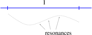
Figure 2. The rescaled resonances for a periodic potential

One can also study what happens below the lines Im$z=-C/L$. Therefore, one considers the function

(1.6) $$\hskip-142.26378pt\Xi(z):=\int_{\mathbb{R}}\frac{dN(\lambda)}{\lambda-z}+e^{-i\arccos(z/2)}$$

defined in the lower half-plane where, the function $z\mapsto\arccos z$ is the analytic continuation to the lower half-plane of the determination taking values in $[-\pi,0]$ over the interval $[-1,1]$.
A study of the behavior of this function on the boundary $\partial\mathbb{C}^{-}$ shows that, on $\mathbb{C}^{-}$, $\Xi$ admits at most a finite number of zeros that are all simple. One proves

Theorem 4.

There exists $C_{0}>0$ and $L_{0}>0$ such that, for $L>L_{0}$,

• the number of resonances of $H_{L}$ in the half-plane $\mathbb{R}+i(-\infty,-C_{0}/L]$ is equal to the number of zeros of $\Xi$;

• to each zero of $\Xi$, say $\tilde{z}$, one can associate a unique resonance, say $z$, that satisfies $|z-\tilde{z}|\lesssim L^{-1}$.

So, by Theorem 3, except for a finite number of resonances that converge to the zeros of $\Xi$, all the resonances of $H_{L}$ converge to the spectrum of $H$.

2. The random case

Let now $V=V_{\omega}$ where $V_{\omega}(n)=\omega_{n}$ and $(\omega_{n})_{n\geq 0}$ are bounded independent and identically distributed random variables. Assume that the common law of the random variables admits a bounded density, say, $g$.
Set $H_{\omega}=-\Delta+V_{\omega}$ on $\ell^{2}(\mathbb{N})$. Let $\sigma(H_{\omega})$ be the spectrum of $H_{\omega}$ and $\Sigma$ be the almost sure spectrum of $-\Delta+V_{\omega}$ acting on $\ell^{2}(\mathbb{Z})$ (see [10]); one knows that

$$\Sigma=[-2d,2d]+\text{supp}\,g$$

One has the following description for the spectra:

• $\omega$-almost surely, $\sigma(H_{\omega})=\Sigma$; the spectrum is purely punctual; it consists of simple eigenvalues associated to exponentially decaying eigenfunctions (Anderson localization, see e.g. [20, 10]); one can prove that the whole spectrum is dynamically localized;

• on $\ell^{2}(\mathbb{N})$, one has (see e.g. [20, 2])

  • $\omega$-almost surely, $\sigma(H_{\omega})=\Sigma\cup K_{\omega}$;

  • $\Sigma$ is the essential spectrum of $H_{\omega}$; it consists of simple eigenvalues associated to exponentially decaying eigenfunctions;

  • the set $K_{\omega}$ is the discrete spectrum of $H_{\omega}$ which may be empty and depends on $\omega$.

2.1. The integrated density of states and the Lyapunov exponent

The integrated density of states is defined by (1.2). It is the distribution function of a probability measure supported on $\Sigma$. As the common law of the random variables $(\omega_{n})_{n\geq 0}$ admits a bounded density, the integrated density of states $N(E)$ is known to be Lipschitz continuous ([20, 10]). Let $\displaystyle n(E)=\frac{dN}{dE}(E)$ be its derivative; it exists for almost every $E$.
One also defines the Lyapunov exponent, say $\rho(E)$ as follows

(2.1) $$\rho(E)=\lim_{L\to+\infty}\frac{1}{L+1}\log\left\|\prod_{n=L}^{0}\begin{pmatrix}E-V_{\omega}(n)&-1\\ 1&0\end{pmatrix}\right\|.$$

For any $E$, $\omega$-almost surely, this limit is known to exist and to be independent of $\omega$ (see e.g. [20, 2]). Moreover, it is positive and continuous for all $E$ and the Thouless formula states that it is the harmonic conjugate of $n(E)$ (see e.g. [4]).

2.2. Resonance free regions

We again start with a description of the resonance free region near the spectrum of $-\Delta$. As in the periodic case, the size of this region will depend on whether an energy belongs to the essential spectrum of $H_{\omega}$ or not. We prove

Theorem 5.

Let $I$ be a compact interval in $(-2,2)$. Then, one has

• there exists $C>0$ such that, $\omega$-a.s., if $I\subset\mathbb{R}\setminus\sigma(H_{\omega})$, then, for $L$ sufficiently large, there are no resonances of $H_{\omega,L}$ in $\{\text{Re}\,z\in I,\ \text{Im}\,z\geq-1/C\}$;

• there exists $C>0$ such that, $\omega$-a.s., if $\{v_{j}\}=\{v_{j}(\omega)\}=\overset{\circ}{I}\cap K_{\omega}=I\cap K_{\omega}$ and $I\cap\Sigma=\emptyset$, then, for $L$ sufficiently large, there exists a unique resonance in $\{\text{Re}\,z\in I,\ \text{Im}\,z\geq-1/C\}$; moreover, this resonance, say $z_{j}$, satisfies (1.3) for some $\rho_{j}=\rho_{j}(\omega)$ independent of $L$.

• if $I\subset\overset{\circ}{\Sigma}$, then, there exists $C>0$ such that, $\omega$-a.s., for $L$ sufficiently large, there are no resonances of $H_{\omega,L}$ in $\{\text{Re}\,z\in I,\ \text{Im}\,z\geq-e^{-2\rho L(1+o(1))})\}$ where $\rho$ is the maximum of the Lyapunov exponent $\rho(E)$ on $I$.

When comparing this result with Theorem 2, it is striking that the width of the resonance free region below $\Sigma$ is much smaller in the random case than in the periodic case. This a consequence of the localized nature of the spectrum i.e. of the exponential decay of the eigenfunction.

2.3. Description of the resonances close to $\Sigma$

We will now see that below the resonance free strip exhibited in Theorem 5 one does find resonances, actually, many of them. We prove

Theorem 6.

Let $I$ be a compact interval in $(-2,2)\cap\overset{\circ}{\Sigma}$. Then, $\omega$-a.s.,

• for any $\kappa\in(0,1)$, one has

  $$\frac{1}{L}\#\left\{z\text{ resonance of }H_{\omega,L}\text{ s.t. Re}\,z\in I,\ \text{Im}\,z\geq-e^{-L^{\kappa}}\right\}\to\int_{I}dN(E);$$

• fix $E\in I$ such that $n(E)>0$; then, for $\delta>0$, there exits $\varepsilon>0$ such that

  $$\liminf_{L\to+\infty}\frac{1}{L}\#\left\{\text{resonances }z\text{ s.t. }\begin{split}\text{ Re}\,z\in[E-\varepsilon,E+\varepsilon],\\ \text{Im}\,z\geq-e^{-2(\rho(E)-\delta)L}\end{split}\right\}>0.$$

The first striking fact is that the resonances are much closer to the real axis than in the periodic case; the lifetime of these resonances is much larger. The resonant states are quite stable with lifetimes that are exponentially large in the width of the random perturbation.
The structure of the set of resonances is also very different from the one observed in the periodic case (see Fig. 2) as we will see now. Let $I$ be a compact interval in $(-2,2)\cap\overset{\circ}{\Sigma}$ and $\kappa\in(0,1)$. Fix $E_{0}\in I$ such that $n(E_{0})>0$.
Let $(z_{i}^{L}(\omega))_{i}$ be the resonances of $H_{\omega,L}$ in $\displaystyle K_{L}:=[E_{0}-\varepsilon,E_{0}+\varepsilon]+i\left[-e^{-L^{\kappa}},0\right]$. We first rescale the resonances: define

(2.2) $$x_{j} =x_{j}^{L}(\omega)=n(E_{0})\,L\,(\text{Re}\,z_{j}^{L}(\omega)-E_{0})$$

$$y_{j} =y_{j}^{L}(\omega)=-\frac{1}{2\rho(E_{0})\,L}\log|\text{Im}\,z_{j}^{L}(\omega)|.$$

Let us note that the scaling of the real and of the imaginary of the resonances are very different. According to the conclusions of Theorem 6, this scaling essentially sets the mean spacing between the real parts of the resonances to $1$ and the imaginary parts to be of order $1$.Consider now the two-dimensional point process $\xi_{L}(E_{0},\omega)$ defined

(2.3) $$\xi_{L}(E_{0},\omega)=\sum_{z_{j}^{L}\in K_{L}}\delta_{(x_{j},y_{j})}.$$

We prove

Theorem 7.

The point process $\xi_{L}$ converges weakly to a Poisson process in $\mathbb{R}\times[0,1]$ with intensity $1$. That is, for any $p\geq 0$, if $(I_{n})_{1\leq n\leq p}$ resp. $(C_{n})_{1\leq n\leq p}$, are disjoint intervals of the real line $\mathbb{R}$ resp. of $[0,1]$, then

$$\lim_{L\to+\infty}\mathbb{P}\left(\left\{\omega;\ \begin{aligned} &\#\left\{j;\begin{aligned} x_{j}(\omega,\Lambda)&\in I_{1}\\ y_{j}(\omega,\Lambda)&\in C_{1}\end{aligned}\right\}=k_{1}\\ &\hskip 28.45274pt\vdots\hskip 56.9055pt\vdots\\ &\#\left\{j;\begin{aligned} x_{j}(\omega,\Lambda)&\in I_{p}\\ y_{j}(\omega,\Lambda)&\in C_{p}\end{aligned}\right\}=k_{p}\end{aligned}\right\}\right)=\prod_{n=1}^{p}e^{-\mu_{n}}\frac{(\mu_{n})^{k_{n}}}{k_{n}!},$$

where $\mu_{n}:=|I_{n}||C_{n}|$ for $1\leq n\leq p$.

Hence, after rescaling the picture of the resonances (see Fig 3) is that of points chosen randomly independently of each other in $\mathbb{R}\times[0,1]$.

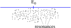
Figure 3. The rescaled resonances for a random potential

This is the analogue of the celebrated result on the Poisson structure of the eigenvalues for a random system (see e.g. [19, 18, 7]) In [11], we proved decorrelation estimates that can be used in the present setting to prove

Theorem 8.

Fix $E_{0}\not=E^{\prime}_{0}$ such that $n(E_{0})>0$ and $n(E^{\prime}_{0})>0$. Then, the limits of the processes $\xi_{L}(E_{0},\omega)$ and $\xi_{L}(E^{\prime}_{0},\omega)$ are stochastically independent.

Due to the rescaling, the above results give a picture of the resonances in a zone of the type

$$E_{0}+L^{-1}\left[-\varepsilon^{-1},\varepsilon^{-1}\right]-i\,\left[e^{-2(1-\varepsilon)\rho(E_{0})L},e^{-2\varepsilon\rho(E_{0})L}\right]$$

For $\varepsilon>0$ small fixed, when $L$ gets large, this rectangle is of a very small width and located very close to the real axis. One can actually bet a picture of the resonances near a line Im$z=e^{-2\rho(E_{0})L\delta}$ for $\delta\in[0,1]$. Though the resonances closest to the real axis play the most important role in scattering (see e.g. [25]), such a picture answers the natural question of what happens deeper in the lower half-plane.
Fix an increasing sequence of scales $\ell=(\ell_{L})_{L}$ such that

(2.4) $$\frac{\ell_{L}}{\log L}\operatornamewithlimits{\to}_{L\to+\infty}+\infty\quad\text{ and }\quad\frac{\ell_{L}}{L}\operatornamewithlimits{\to}_{L\to+\infty}0.$$

Fix $x_{0}\in[0,1]$ and $E_{0}\in I$ so that $\nu(E_{0})>0$. Let $(z_{i}^{L}(\omega))_{i}$ be the resonances of $H_{\omega,L}$ in $\displaystyle\tilde{K}_{L}:=E_{0}+\ell_{L}^{-1}\left[-\varepsilon^{-1},\varepsilon^{-1}\right]+i\left[-e^{-\ell_{L}},0\right]$. Note that $\tilde{K}_{L}$ is much larger than $K_{L}$. We first rescale the resonances using the sequence $(\ell_{L})_{L}$: define

(2.5) $$x_{j} =x_{j}^{\ell_{L}}(\omega)=n(E_{0})\,\ell_{L}\,(\text{Re}\,z_{j}^{L}(\omega)-E_{0}),$$

$$y_{j} =y_{j}^{\ell_{L}}(\omega)=-\frac{1}{2\,\rho(E_{0})\,\ell_{L}}\left[2\,\rho(E_{0})\,L\,x_{0}+\log|\text{Im}\,z_{j}^{L}(\omega)|\right].$$

Note that if $\ell_{L}=L$, we recover (2.2) up to a shift for the imaginary part. The scaling introduced in (2.5) is different from the one introduced in (2.2). Here, we look at a window of size $\ell^{-1}_{L}$ around $E_{0}$ is the real parts (it is thus much larger than the $L^{-1}$ window considered in (2.2)); but, in the imaginary part, on a logarithmic scale we look at a window of size $\ell_{L}$ around the point $-2\rho(E_{0})x_{0}L$ (this is much smaller than the window of size $L$ considered in (2.2)-(2.3)). This covariant scaling of the real and imaginary parts of the resonances is the correct analogue of the covariant scaling introduced in [7] for the eigenvalues and localization centers of a random operator in the localized phase. Consider now the two-dimensional point process $\xi_{L,\ell}(x_{0},E_{0},\omega)$ defined by

(2.6) $$\xi_{L,\ell}(x_{0},E_{0},\omega)=\sum_{z_{j}^{L}\in K_{L}}\delta_{(x_{j},y_{j})}.$$

We prove

Theorem 9.

For $x_{0}\in[0,1]$ and $E_{0}\in I$ so that $\nu(E_{0})>0$, the point process $\xi_{L}(x_{0},E_{0},\omega)$ converges weakly to a Poisson process in $\mathbb{R}\times\mathbb{R}$ with intensity $1$.

So we see that the local picture of the rescaled resonances around the point $E_{0}$ near the line Im$z=-ie^{-2\rho(E_{0})x_{0}L}$ is essentially independent of $E_{0}$ and $x_{0}$. A value of particular interest is $x_{0}=0$. In this case, we look at resonances lying at a distance of order $e^{-\ell_{L}}$ from the real axis (thus, much further away that the resonances considered in Theorem 7). By condition (2.4), we can get a precise description of the resonances lying almost at a polynomial distance to the real axis.For the processes $(\xi_{L}(x_{0},E_{0},\omega))_{x_{0},E_{0}}$, one gets an asymptotic independence result analogous to Theorem 8, namely,

Theorem 10.

Fix $E_{0}$ and $E^{\prime}_{0}$ such that $n(E_{0})>0$ and $n(E^{\prime}_{0})>0$ and $x_{0}$ and $x^{\prime}_{0}$ such that $(x_{0},E_{0})\not=(x^{\prime}_{0},E^{\prime}_{0})$.
Then, the limits of the processes $\xi_{L}(x_{0},E_{0},\omega)$ and $\xi_{L}(x^{\prime}_{0},E^{\prime}_{0},\omega)$ are stochastically independent.

One can get a number of other statistics using the techniques developed for the study of the spectral statistics of the eigenvalues of a random system in the localized phase (see [8, 7]).

2.4. The description of the low lying resonances

One can also study what happens below the lines Im$z=-e^{-\log^{\alpha}L}$ (for $\alpha>1$). As we will see the picture is quite different from that obtained for the periodic case (see section 1.4).
To state the result, it will be convenient to change the notation slightly and to write the operator $H_{\omega,L}$ as

(2.7) $$\tilde{H}_{\omega,L}=-\Delta+\tilde{V}_{\omega,L}\text{ where }V_{\omega,L}=\begin{cases}\omega_{L-n}&\text{ if }n\in\llbracket 0,L\rrbracket,\\ 0&\text{ if not}.\end{cases}$$

As the random variables $(\omega_{n})_{n\geq 0}$ are i.i.d, the families $(H_{\omega,L})_{\omega}$ and $(\tilde{H}_{\omega,L})_{\omega}$ have the same distribution.
On $\ell^{2}(\mathbb{Z})$, consider the following random operator

(2.8) $$\tilde{H}_{\omega}=-\Delta+\tilde{V}_{\omega}\text{ where }V_{\omega}=\begin{cases}\omega_{-n}&\text{ if }n\leq 0,\\ 0&\text{ if }n>0.\end{cases}$$

The resonances (in the sense of Theorem 1) of this operator were studied in [15, 14]. It was in particular shown that, below any line Im$\,z=-1/C$, $\tilde{H}_{\omega}$ has at most finitely many resonances.
We show

Theorem 11.

Fix $\alpha>1$. Then, $\omega$-almost surely, there exists $L_{0}>0$ and $C_{0}>0$ such that, for $L>L_{0}$,

• the number of resonances of $\tilde{H}_{\omega,L}$ in the half-plane $\displaystyle\mathbb{R}+i\left(-\infty,-e^{-\log^{\alpha}L}\right]$ is equal to the number of resonances of $\tilde{H}_{\omega}$ in the same half-plane;

• to each resonance of $\tilde{H}_{\omega}$ in this half-plane, say $\tilde{z}$, one can associate a unique resonance of $\tilde{H}_{\omega,L}$, say $z$, that satisfies $|z-\tilde{z}|\leq e^{-L/C_{0}}$.

Hence, we see that, in opposition to the periodic case, not all resonances except finitely many of them converge to the spectrum $H_{\omega}$.
It is interesting to note that the result of Theorem 11 stays true on the (larger) half-plane $\displaystyle\mathbb{R}+i\left(-\infty,-e^{-L^{\beta}}\right]$ (for $\beta\in(0,1)$).
Finally, let us say that one can combine Theorem 9 and 11 to recover the results of [15, 14] on behavior of the average density of resonances of $\tilde{H}_{\omega}$ at a distance $y$ from the real axis in the limit $y\to 0$.

References

- [1] F. Barra and P. Gaspard. Scattering in periodic systems: from resonances to band structure. J. Phys. A, 32(18):3357–3375, 1999.
- [2] R. Carmona and J. Lacroix. Spectral theory of random Schrödinger operators. Probability and its Applications. Birkhäuser Boston Inc., Boston, MA, 1990.
- [3] A. Comtet and C. Texier. On the distribution of the Wigner time delay in one-dimensional disordered systems. J. Phys. A, 30(23):8017–8025, 1997.
- [4] H. L. Cycon, R. G. Froese, W. Kirsch, and B. Simon. Schrödinger operators with application to quantum mechanics and global geometry. Texts and Monographs in Physics. Springer-Verlag, Berlin, study edition, 1987.
- [5] W. G. Faris and W. J. Tsay. Scattering of a wave packet by an interval of random medium. J. Math. Phys., 30(12):2900–2903, 1989.
- [6] W. G. Faris and W. J. Tsay. Time delay in random scattering. SIAM J. Appl. Math., 54(2):443–455, 1994.
- [7] F. Germinet and F. Klopp. Spectral statistics for random Schrödinger operators in the localized regime. ArXiv http://arxiv.org/abs/1011.1832, 2010.
- [8] F. Germinet and F. Klopp. Spectral statistics for the discrete Anderson model in the localized regime. In N. Minami, editor, Spectra of random operators and related topics, 2011. To appear. ArXiv http://arxiv.org/abs/1004.1261.
- [9] F. W. King. Hilbert transforms. Vol. 1, volume 124 of Encyclopedia of Mathematics and its Applications. Cambridge University Press, Cambridge, 2009.
- [10] W. Kirsch. An invitation to random Schrödinger operators. In Random Schrödinger operators, volume 25 of Panor. Synthèses, pages 1–119. Soc. Math. France, Paris, 2008. With an appendix by Frédéric Klopp.
- [11] F. Klopp. Decorrelation estimates for the discrete Anderson model. Comm. Math. Phys., 303(1):233–260, 2011.
- [12] F. Klopp. Resonances for “large” ergodic systems i: one-dimensional systems. In preparation, 2011.
- [13] T. Kottos. Statistics of resonances and delay times in random media: beyond random matrix theory. J. Phys. A, 38(49):10761–10786, 2005.
- [14] H. Kunz and B. Shapiro. Resonances in a one-dimensional disordered chain. J. Phys. A, 39(32):10155–10160, 2006.
- [15] H. Kunz and B. Shapiro. Statistics of resonances in a semi-infinite disordered chain. Phys. Rev. B, 77(5):054203, Feb 2008.
- [16] I. M. Lifshits, S. A. Gredeskul, and L. A. Pastur. Introduction to the theory of disordered systems. A Wiley-Interscience Publication. John Wiley & Sons Inc., New York, 1988. Translated from the Russian by Eugene Yankovsky [E. M. Yankovskiĭ].
- [17] M. Merkli and I. M. Sigal. A time-dependent theory of quantum resonances. Comm. Math. Phys., 201(3):549–576, 1999.
- [18] N. Minami. Local fluctuation of the spectrum of a multidimensional Anderson tight binding model. Comm. Math. Phys., 177(3):709–725, 1996.
- [19] S. A. Molchanov. The local structure of the spectrum of a random one-dimensional Schrödinger operator. Trudy Sem. Petrovsk., (8):195–210, 1982.
- [20] L. A. Pastur and A. Figotin. Spectra of random and almost-periodic operators, volume 297 of Grundlehren der Mathematischen Wissenschaften [Fundamental Principles of Mathematical Sciences]. Springer-Verlag, Berlin, 1992.
- [21] B. Pavlov. Nonphysical sheet for perturbed Jacobian matrices. Algebra i Analiz, 6(3):185–199, 1994.
- [22] C. Texier and A. Comtet. Universality of the Wigner Time Delay Distribution for One-Dimensional Random Potentials. Physical Review Letters, 82:4220–4223, May 1999.
- [23] M. Titov and Y. V. Fyodorov. Time-delay correlations and resonances in one-dimensional disordered systems. Phys. Rev. B, 61(4):R2444–R2447, Jan 2000.
- [24] P. van Moerbeke. The spectrum of Jacobi matrices. Invent. Math., 37(1):45–81, 1976.
- [25] M. Zworski. Quantum resonances and partial differential equations. In Proceedings of the International Congress of Mathematicians, Vol. III (Beijing, 2002), pages 243–252, Beijing, 2002. Higher Ed. Press.
- [26] M. Zworski. Resonances in physics and geometry. Notices Amer. Math. Soc., 46(3):319–328, 1999.