Criticality in conserved dynamical systems: Experimental observation vs. exact properties

Abstract

Conserved dynamical systems are generally considered to be critical. We study a class of critical routing models, equivalent to random maps, which can be solved rigorously in the thermodynamic limit. The information flow is conserved for these routing models and governed by cyclic attractors. We consider two classes of information flow, Markovian routing without memory and vertex routing involving a one-step routing memory. Investigating the respective cycle length distributions for complete graphs we find log corrections to power-law scaling for the mean cycle length, as a function of the number of vertices, and a sub-polynomial growth for the overall number of cycles.

When observing experimentally a real-world dynamical system one normally samples stochastically its phase space. The number and the length of the attractors are then weighted by the size of their respective basins of attraction. This situation is equivalent to ‘on the fly’ generation of routing tables for which we find power law scaling for the weighted average length of attractors, for both conserved routing models. These results show that critical dynamical systems are generically not scale-invariant, but may show power-law scaling when sampled stochastically. It is hence important to distinguish between intrinsic properties of a critical dynamical system and its behavior that one would observe when randomly probing its phase space.

Power law scaling is observed in many real-world systems, like the distribution of neural avalanches in the brain. In statistical physics all critical systems, at the point of a second-order phase transition, show power law scaling. Power law scaling is hence commonly attributed to criticality, but it is an open question to which extend this relation is satisfied for complex dynamical systems. There is, in addition, a difference between the distribution an observer may be able to sample and the exact properties of the underlying dynamical system. An observer will sample in general the number and the size of attractors as weighted by size of their respective basins of attraction. Here we investigate critical models for information routing and show that the number and the length of attractors does not obey power law scaling, while, on the other hand, an external observer, sampling the weighted distribution, would find power law scaling. We hence conclude that drawing conclusions from experimentally observed power law scaling needs to take into account the implicitly employed sampling procedures.

 

I Introduction

The propagation of perturbations is a central notion in dynamical system theory. One speaks of a frozen state when a perturbation tends to die out, on the average, during the course of time evolution and of a chaotic state when perturbations tend to spread out derrida86 ; gros08 . A given class of dynamical systems may change from frozen to chaotic behavior as a function of parameters, being critical right at the transition point.

At criticality, information is on the average conserved tsuchiya00 , as one can regard a perturbation of a state as the information about the persistence of small differences. A well studied example of a critical dynamical system is the Kauffman net with connectivity $K=2$, an example of a random Boolean network kauffman69 ; aldana03 ; drossel08 . In statistical mechanics critical systems are generically scale invariant reichl09 , and it has been widely assumed that this statement would also hold for critical dynamical systems. Indeed numerical simulations seemed to support scaling in critical Boolean networks, notably a $\sqrt{N}$ scaling for the number of attractors as a function of the number of vertices $N$ had been proposed kauffman69 ; aldana03 .

An important clarification then came with the exact proof that the number of attractors actually grows faster than any power of $N$, and that the results of the numerical simulations suffered from systematic undersampling of phase space samuelsson03 . It could be shown, on the other side, that the number of frozen and the number of relevant nodes in a large class of critical Boolean networks obey power law scaling mihaljev06 . The situation is then that certain properties of critical dynamical systems, at least for the case of random Boolean networks, obey power law scaling while others do not. It is hence important to investigate the possible occurrence of scaling in different classes of dynamical systems.

We study a class of dynamical systems describing the transport of conserved quantities on network structures, that is quantities which cannot be multiplied or separated into smaller parts during the transport between network nodes. We denote such a process a routing process, since only one node is active at each time step, the one containing the transmitted quantity. A routing process can be seen alternatively as the transport of perturbations between network elements and as such represents a critical process because the perturbation neither spreads out through the entire network nor does it die out. A routing process initiated from a given network node will eventually follow a limiting cycle, thus the total number of nodes affected by the perturbation will be a finite fraction of the whole network. Hence, a routing process satisfies the conditions needed for it to be considered as a critical dynamical process luque2000 .

Transport on networks, like the spreading of rumors Moreno04 and diseases klovdahl85 in social networks or the flow of capital in financial networks fronczak11 has been studied intensively, indeed transport constitutes a basic process in biology quite in general anderson95 , as well as in sociology and technical applications. In many cases the quantity transported is not conserved, e.g. when considering the spreading of rumors in social networks. Routing processes, investigated here, model the transport of a conserved quantity, like conserved information packages. Information packages are sent from node to node and are routed at every vertex, as illustrated in Fig. 1. A routing process eventually ends up in one of the cyclic attractors, the members of the attractors benefiting hence from a continuous flow of information arriving from the respective basins of attraction. We have shown previously that the geometric arrangement of the attractors on the network gives rise in the thermodynamic limit to a non-trivial distribution for the information centrality, which measures the number of attractors intersecting at a given vertex markovic09 .

We present here the solution for two types of routing models, Markovian routing in the absence of a routing memory and vertex routing in the presence of an one-step memory. The solutions are asymptotically exact in the thermodynamic limit $N\to\infty$, they can be evaluated for large networks containing thousands to millions of sites. We present results for the scaling behavior of the overall number of attractors and for the mean of the cycle length distribution. We find, that the number of cycles increases as $\log(N)$ and that the mean cycle length scales like $\sqrt{N}/\log(N)$ and $N/\log(N)$ respectively for the model without and with routing memory.

We also derive rigorous results for the case of stochastic sampling of phase space, which yields a cycle length distribution weighted by the size of the respective basins of attraction. This kind of ‘on the fly’ sampling is generically equivalent to an experimental observation of a real-world dynamical system. We find power law scaling for on-the-fly sampling, logarithmic corrections are absent. We conclude that real-world investigations of scaling in complex dynamical systems, like the brain, need to be interpreted carefully.

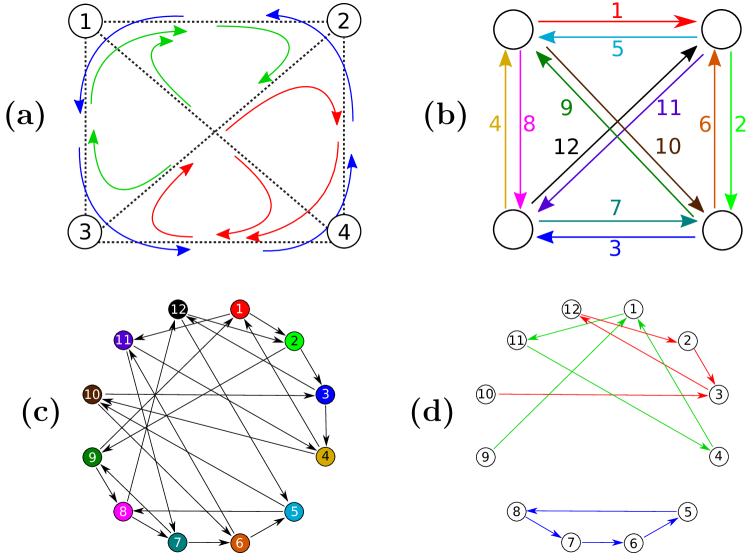
Figure 1: Vertex routing dynamics for a $N=4$ complete graph (a) A realization of the routing tables. Routing through the first vertex follows $T_{312}=T_{213}=T_{214}=1$, with all other $T_{i1j}$ vanishing. There are three cyclic attractors, namely $(123)$, $(243)$ and $(1342)$. (b) Enumeration of all $N(N-1)=12$ directed edges, the phase-space elements. (c) The corresponding phase-space graph. (d) The same realization of the routing table as in (a), now in terms of the phase-space graph.

II Models

The two classes of models we consider differ with respect to the absence/presence of a routing memory. The phase space volume $\Omega$ is respectively linear and quadratic in the number of vertices $N$.

• For the Markovian model the selection of the next active vertex is independent of the previous state meyn93 . At every point in time only one vertex is active, the vertex with the information package. The phase space is hence identical with the collection of vertices; $\Omega=N$;

• For the vertex routing model the phase space is given by the collection of directed links; $\Omega=N(N-1)$. At every point in time one directed link is active, the link currently transporting the information package, compare Fig. 1.

In both setups the routing of information packages is realized through static routing tables. For every incoming edge the routing table specifies an allowed outgoing edge. A vertex $k$ will transmit an information package, which was received from a vertex $j$, to a specific neighboring vertex $i$. The vertex routing table $\hat{T}$ corresponds to a tensor of binary elements $T_{ikj}=(\hat{T})_{ikj}\in\{0,1\}$,

$$T_{ikj}\ =\ \left\{\begin{array}[]{rll}0&\quad\hbox{no\ routing\ allowed}&\\ 1&\quad\hbox{routing\ from}&\vec{e}_{jk}\hbox{\ to\ }\vec{e}_{ki}\end{array}\right.~{},$$ (1)

where $\vec{e}_{jk}$ denotes a directed edge from vertex $j$ to vertex $k$. An example of a routing table for a four-site network is presented in Fig. 1. In Fig. 1 (a) allowed routing paths are color coded and mapped to a four-site network. The complete phase space of this network is obtained by representing each edge (Fig. 1 (b)) as a node in an iterated graph which is shown in Fig. 1 (c). Here each node corresponds to a same colored and numbered edge shown in Fig. 1 (b). In Fig. 1 (d) we show again a single realization of routing tables, but now in the iterated phase space graph. The edges of the phase space graph shown correspond to allowed routing directions, that is, to non-zero entries of the routing table $\hat{T}$.

We consider here critical models, viz. models where the number of information packages is conserved. When the information is received along edge $\vec{e}_{jk}$, it can hence be transmitted along only one outgoing edge $\vec{e}_{ki}$,

$$\sum_{i}T_{ikj}=1,\qquad\sum_{ij}T_{ikj}=z_{k}~{},$$ (2)

the non-zero entries of the routing table are drawn randomly. Here $z_{k}$ is the degree of vertex $k$, which is $N-1$ for fully connected networks considered here. For the Markovian model the routing table $T_{ikj}$ is independent of $j$, that is, routing depends only on the node which received the information package and not on the direction along the information was received.

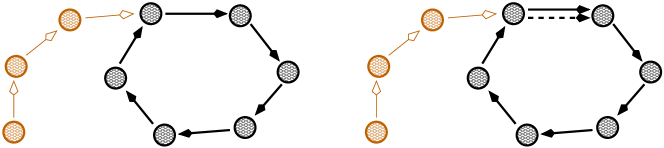
Figure 2: Random walks through configuration space for the Markovian model (left) and for the vertex routing model (right). In order to find an attractor independent of the size of their basins of attraction (light color) one needs to close the path at the respective starting points. The probability to find a given attractor is, on the other side, proportional to the size of its basin of attraction for stochastic ‘on the fly’ sampling of phase space.

III Cycle length distribution

The dynamics consists of random walks through configuration space, as illustrated in Fig. 2. One can hence adapt the considerations gros08 , used for solving the Kauffman network for large connectivity $K\to\infty$, in order to solve the vertex routing model analytically. In addition to the previously derived expression for cycle length distribution in the case of the Markovian model markovic09 , we present here the solution of the vertex routing model.

The general expression for the average number of cycles $\langle C_{L}\rangle$ of length $L$ is given by

$$\langle C_{L}\rangle_{N}(r)=\frac{N(N-1)^{r}}{L(N-1)^{r+1}}~{}q_{r}(t=L-1),$$ (3)

where $r=0$ for the Markovian model and $r=1$ for the vertex routing model. Here the factor $1/L$ cancels overcounting of a cycle of length $L$, while the factor $N(N-1)^{r}$ is the number of phase space elements, that is the number of possible starting elements. The factor $1/(N-1)^{r+1}$ gives the probability to close the cycle exactly at the starting phase space element. For the Markovian model the probability to close the cycle at the starting node is inversely proportional to the number of neighbors, whereas in the vertex routing model this probability is inversely proportional to the squared number of neighbors as the initial edge has to be matched for closing the path (see Fig. 2). The $q_{r}(t=L-1)$ is the probability that a path containing $L$ nodes is still open. At a time step $t=0,1,\ldots$, we have already visited $t$ nodes. Thus, a probability that the next node in the sequence was already visited is $t/(N-1)$. For the trajectory to enter a cycle, the routing has to retrace the existing path. The probability for this to happen is $1/(N-1)^{r}$. The relative probability of closing the path at next time step is then $\rho_{r}(t)=t/(N-1)^{r+1}$. This relation constitutes an approximation, for finite $N<\infty$, in the case of the vertex routing model, as self-intersecting paths are neglected.

The probability of still having an open path after $t+1$ steps is

$$q_{r}(t+1)=q_{r}(t)(1-\rho_{r}(t)).$$ (4)

Expanding the equation till the term $q_{r}(1)=1$ and substituting the expression for relative probability one obtains

$$q_{r}(t)=\frac{((N-1)^{r+1}-1)!}{(N-1)^{(r+1)(t-1)}((N-1)^{r+1}-t)!}~{}.$$ (5)

Substituting (5) in (3) for the Markovian model, given by $r=0$, one finds

$$\langle C_{L}\rangle_{m}(N)=\frac{N!}{L(N-1)^{L}(N-L)!}$$ (6)

for the average number of cycles of length $L$. For the vertex routing model, given by $r=1$, the average number of cycles is

$$\langle C_{L}\rangle_{v}(N)=\frac{N((N-1)^{2})!}{L(N-1)^{2L-1}((N-1)^{2}+1-L)!}~{},$$ (7)

Note that for the Markovian model the cycle length $L$ falls within a range $\{2,N\}$, while $L\in\{2,(N-1)^{2}+1\}$ for the vertex routing model.

Relation (7) is an approximation to the average number of cycles as it doesn’t take into account corrections for self intersecting paths. These corrections drop however as ${1}/{N}$ and can be neglected in the thermodynamic limit. Furthermore, the graph of the phase space elements (see Fig. 1 (c)) is not fully connected and thus not Hamiltonian for arbitrary network size $N$, which means that cycle visiting every element of the phase space do in general not exist. Formulas (6) and (7) are based on a mapping to random maps and can be generalized to the case of routing on $NK$ networks.

The probability of observing a cycle of length $L$ is obtained by dividing the average number of cycles of length $L$ from (6) and (7) by the total number of cycles in a single realization of the routing table which is given as

$$\langle n\rangle_{v,m}=\sum_{L}\,\langle C_{L}\rangle_{v,m}~{}.$$

We denote with

$$\rho_{m,v}(L,N),\qquad\quad\sum_{L}\rho_{m,v}(L,N)=1$$

the normalized cycle length distributions for the Markovian (m) and for the vertex routing model (v), Note that substituting $N$ by $(N-1)^{2}+1$ in (6) one obtains for large N the approximate scaling relation

$$\langle C_{L}\rangle_{v}(N)\ \sim\ \langle C_{L}\rangle_{m}((N-1)^{2}+1)$$ (8)

between the number of cycles of the vertex routing and the Markovian model, $\langle C_{L}\rangle_{v}$ and $\langle C_{L}\rangle_{m}$.

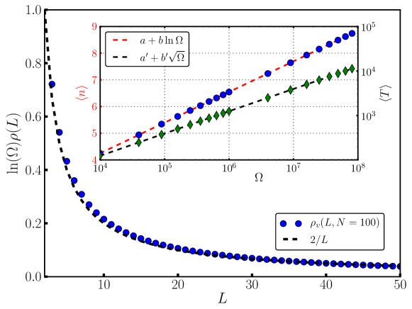
Figure 3: The cycle length distributions $\rho_{v}(L)$, rescaled by $\log(\Omega)$, for the vertex routing model. The dashed line, $2/L$, represents the large-$N$ and small-$L$ limiting behavior. In the inset two quantities are plotted as a function of the phase space volume $\Omega$. The average number of cycles $\langle n\rangle$ (see Eq. (9), filled blue circles, log-linear plot) and the expected total cycle length $\langle T\rangle$ (see Eq. (10), green filled diamonds, log-log plot). Also included are fits using $a+b\ln\Omega$ (red dashed line), with $a=-0.345(3)$ and $b=0.4988(2)$, and using $a^{\prime}+b^{\prime}\sqrt{\Omega}$ (black dashed line) with $a^{\prime}=-0.3311(5)$ and $b^{\prime}=1.25331\pm 2\cdot 10^{-7}$. The coefficient of determination is $R^{2}=1.0$ in both cases, within the numerical precision.

Table 1: Scaling relations, as a function of the number of vertices $N$, for the number of cycles and for the mean of the cycle length distribution, respectively for vertex routing (v) and the Markovian (m) model. The routing table distribution is either quenched (exact result) or generated on the fly, as it corresponds to a stochastic sampling of phase space. Only relative quantities can be evaluated for on the fly dynamics.

		quenched	on the fly
(v)	number of cycles	$\log(N)$	–
	mean cycle length	$N/\log(N)$	$N$
(m)	number of cycles	$\log(N)$	–
	mean cycle length	$\sqrt{N}/\log(N)$	$\sqrt{N}$

IV Results

The analytic expressions (6) and (7) for the number of attractors are valid for quenched dynamics gros08 , viz for fixed routing tables. One can, in addition, evaluate the number of cycles obtained when randomly sampling phase space, which corresponds to generating the routing tables on the fly. The corresponding results will be discussed in Sect. IV.2.

IV.1 Quenched dynamics

Evaluating numerically the number of cycles (6) and (7) we find, see inset of Fig. 3, that the total number of attractors

$$\langle n\rangle_{v,m}=\sum_{L}\,\langle C_{L}\rangle_{v,m}$$ (9)

growth logarithmically, as a function of phase space volume $\Omega$. This result is consistent with a direct evaluation of the number of attractors for random maps kruskal54 . The total number of cycles hence grows slower than any polynomial of the number of vertices $N$, in contrast to critical Kauffman models, where it grows faster than any power of $N$ samuelsson03 .

The normalized cycle length distributions $\rho_{v,m}(L)=\langle C_{L}\rangle_{v,m}/\langle n\rangle_{v,m}$ thus scale as $1/\log(\Omega)$, due to the divisor $\langle n\rangle_{v,m}$. The rescaled distributions $\log(\Omega)\rho_{v,m}(L)$ approach the thermodynamic limit rapidly, compare Fig. 3. For small cycle lengths $L$ the limiting functional form of the rescaled distributions is $2/L$, while for large $L\rightarrow L_{max}$ it falls off as $(1-L/L_{max})^{(L-L_{max}-1/2)}{\rm e}^{-L}$. The limiting behavior of $\log(\Omega)\rho_{v,m}(L)$ is identical for both models, due to the intermodel scaling relation (8).

The total cycle length, viz. the combined length of all cyclic attractors present for a given system size $N$, is on the average

$$\langle T\rangle_{v,m}=\sum_{L}L\langle C_{L}\rangle_{v,m}~{}.$$ (10)

The total cycle length follows a polynomial growth as the function of phase space volume $\Omega$ (see the inset of Fig. 3). This algebraic dependence of the total cycle length can be obtained analytically by generalizing the analysis kruskal54 for the $N\to\infty$ limiting behavior of the mean cycle length (9) to $\langle T\rangle_{v,m}$.

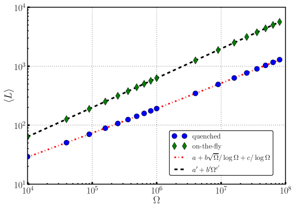
Figure 4: Log-log plot, as a function of the phase space volume $\Omega$, of the mean cycle lengths $\langle L\rangle_{v,\tilde{v}}$, see Eq. (11), for the vertex routing with quenched dynamics ($\langle L\rangle_{v}$, blue circles) and the vertex routing with on the fly dynamics ($\langle L\rangle_{\tilde{v}}$, green diamonds). The dashed lines are fits using $a+b\sqrt{\Omega}/\log(\Omega)+c/\log(\Omega)$ and $a^{\prime}+b^{\prime}\Omega^{c^{\prime}}$ respectively, with $a=8.1(8)$, $b=2.6035(9)$, $c=-69(9)$, and $a^{\prime}=1.3319(3)$, $b^{\prime}=0.406(5)$, $c^{\prime}=0.5\pm 9\cdot 10^{-8}$. The coefficient of determination is $R^{2}=1.0$ in both cases, within the numerical precision.

The determination of the scaling behavior is somewhat more subtle for the mean cycle length (see Fig. 4).

$$\langle L\rangle_{v,m}=\frac{\langle T\rangle_{v,m}}{\langle n\rangle_{v,m}}=\sum_{L}L\rho_{v,m}(L)$$ (11)

We find that the functional dependence on the phase space volume is best reproduced by $a+b\sqrt{\Omega}/\log(\Omega)+c/\log(\Omega)$, where $a,\,b,\,c$ are free parameters, which fits the data by about one order of magnitude better than a pure power law Ansatz $a^{\prime}+b^{\prime}\,\Omega^{c^{\prime}}$. This dependence is obtained by keeping the fastest growing terms of mean cycle length as $\Omega\rightarrow\infty$. Note that $a$, and respectively $a^{\prime}$, are finite size corrections not obtainable when evaluating analytically the scaling of (9) and (10) separately. Interestingly, log-corrections to power law scaling have been studied also in sandpile models at the upper critical dimension lubeck98 and in epidemic percolation janssen03 . An overview of the obtained scaling relations is given in Table 1, where ‘quenched dynamics’ denotes the results for quenched distributions of routing tables (exact result). Note that in Figs. 3 and 4 we present only the data for the vertex routing model as it completely overlaps for large phase spaces $\Omega$, due to the scaling (8), with the results for the Markovian model.

IV.2 Stochastic sampling of phase space

In addition to working with predetermined (quenched) vertex routing tables one can generate dynamics ‘on the fly’ without explicitly creating initially routing tables for all vertices of the network. For this kind of dynamics, which correspond to a stochastic sampling of phase space, a routing for a given vertex is selected only when the trajectory visits this vertex. A cyclic attractor is then found when one state of the phase space (edge or node) is visited more then once. The probability to find a cycle is hence weighted by the size of its basin of attraction.

The probability of observing a closed cycle of length $L$ in a randomly generated path of length $t$ after a total number of $t$ routing steps is

$$p(L|~{}t)=\frac{\Theta(t-L)\Theta(L-2)}{t-1}~{},$$ (12)

where $\Theta(x)$ is the Heaviside step function with $\Theta(0)=1$. The joint probability distribution $P(L,t)$ is given as $P(L,t)=p(L|~{}t)p_{t}$, where $p_{t}=q_{t}\rho_{t}$ is the probability of closing a cycle at the next time step $t+1$. Then, the probability of generating a cycle of length $L$ becomes simply the sum over all possible path lengths, with the maximum path length $t_{\mathrm{max}}=N$ for the Markovian routing and $(N-1)^{2}+1$ for routing with memory. Thus, the probability to find an L-cycle is

$$\tilde{\rho}_{v}(L,N)=\sum_{t=L}^{L_{max}}\frac{((N-1)^{2})!}{(N-1)^{2t}((N-1)^{2}+1-t)!}~{},$$

where we denoted with $\tilde{\rho}_{v}(L,N)$ the weighted cycle length distribution for the vertex routing model, viz the cycle length distribution for on-the-fly dynamics. An analogous relation holds for the Markovian model. By generalizing the scaling relation (8) one finds $\tilde{\rho}_{v}(L,N)=\tilde{\rho}_{m}(L,(N-1)^{2}+1)$ and consequently $\langle L\rangle_{\tilde{v}}(N)=\langle L\rangle_{\tilde{m}}((N-1)^{2}+1)$, where $\tilde{\rho}_{m}$ denotes the weighted cycle length distributions for the Markovian model.

Fitting the data, as shown in Fig. 4 for the vertex routing model, with and without log-corrections, we find evidence for a scaling $\sim{N}$ and $\sim\sqrt{N}$ for the mean cycle lengths of the vertex routing and the Markovian model respectively with on-the-fly dynamics. Note that the overall number of cycles cannot be obtained when routing on the fly, only relative quantities can be evaluated.

V Discussion

For Boolean networks the phase space volume $\Omega$ is $2^{N}$ and hence grows exponentially with the number of vertices $N$. The fact samuelsson03 , that the number of attractors grows faster than any power of $N$ could in principle be related to the exponential growth of the phase space volume. Our results however show, that the critical properties of the Kauffman networks for connectivity $Z=2$, and of the vertex routing models considered here are not related. The scaling $\sim\log(\Omega)$ valid for vertex routing models would imply a polynomial scaling with the system size

$$\log(\Omega)\ \sim\ N,\qquad\quad\Omega=2^{N}$$

for critical Kauffman nets, which is however not observed samuelsson03 . Our results hence indicate that scaling in critical dynamical systems may generically be non-universal, depending on the details of the microscopic dynamics.

We also note that other properties of critical dynamical systems, like the scaling of the number of frozen or relevant nodes for critical Boolean networks mihaljev06 , may show highly non-trivial behavior. For the case of vertex routing models one may define a measure of centrality, information centrality, determined by the number of attractors intersecting a given vertex, which scales to a non-trivial limiting distribution in the thermodynamic limit markovic09 .

Our results may also be seen in the context of the surge in interests in modelling gros09 ; markovic10 and in experimentally investigating ringach09 ; petermann09 the spontaneous neural dynamics of the brain. The observation of power law scaling relations eguiluz05 has been interpreted as evidence of a critical self-organized neural state chialvo10 . The power law scaling in neural activity was observed in spite of strong sub-sampling of neural avalanches resulting from small number of electrodes relative to total number of neurons within the cortex. Priesemann and colleges priesemann2009 have recently demonstrated that sub-sampling of critical avalanches results in the loss of power law scaling, thus suggesting different causes of the power law scaling of neural avalanches observed in various experiments in spite of low number of electrodes, used to record neural activity, compared to a total number of neurons.

Our results suggest, to some extent, that there is no universal relation in dynamical systems theory between criticality and power law scaling and that scaling is generically dependent on the observation modus. The unbiased statistics of a certain property, like the number of attractors or avalanches, may differ from a statistics obtained via stochastic sampling ($\rho_{v,m}(L)$ and $\tilde{\rho}_{v,m}(L)$ in our case). The later will in general be dependent on the size of the respective basins of attraction of the dynamical process considered, viz of a cycle or an avalanche. For the case of the vertex routing models studied here we found logarithmic corrections to power law scaling for the unbiased, quenched statistics and pure power law scaling for stochastic on the fly sampling. We conclude that experimental observations of real-world systems, when investigating scaling, need to be interpreted carefully.

References

- (1) B. Derrida and Y. Pomeau, Random networks of automata: a simple annealed approximation, EPL 1, 45 (1986).
- (2) C. Gros, Complex and Adaptive Dynamical Systems, A Primer, Springer (2008, second edition 2010).
- (3) T. Tsuchiya and M. Katori, Proof of breaking of self-organized criticality in a nonconservative Abelian sandpile model, Phys. Rev. E, 61, 2 (2000).
- (4) S.A. Kauffman, J. Theor. Biol. 22, 437 (1969).
- (5) M. Aldana, S. Coppersmith and L.P. Kadanoff, Boolean dynamics with random couplings, Perspectives and Problems in Nonlinear Science 93, 23 (2003).
- (6) B. Drossel, Random boolean networks, Reviews of nonlinear dynamics and complexity 1 69, (2008).
- (7) L.E. Reichl, A modern course in statistical physics, Vch Pub (2009).
- (8) B. Samuelsson and C. Troein, Superpolynomial growth in the number of attractors in Kauffman networks, PRL 90, 98701 (2003).
- (9) T. Mihaljev and B. Drossel, Scaling in a general class of critical random Boolean networks, Phys. Rev. E 74, 046101 (2006).
- (10) B. Luque and R.V. Solé, Lyapunov exponents in random Boolean networks, Physica A: Statistical Mechanics and its Applications, 284, 33 (2000)
- (11) Y. Moreno, M. Nekovee and A.F. Pacheco, Dynamics of rumor spreading in complex networks, Phys. Rev. E 69, 6 (2004)
- (12) A.S. Klovdahl, Social networks and the spread of infectious diseases: The AIDS example, Social Science & Medicine 21, 11 (1985)
- (13) A. Fronczak and P. Fronczak, Statistical mechanics of the international trade network, arXiv:1104.2606v1, (2011)
- (14) J.A. Anderson, An Introduction to Neural Networks Cambridge, Mass., MIT Press (1995)
- (15) D. Marković and C. Gros, Vertex routing models, New Journal of Physics 11, 7 (2009)
- (16) S.P. Meyn and R.L. Tweedie, Markov Chains and Stochastic Stability Springer (1993)
- (17) M.D. Kruskal, The expected number of components under a random mapping function, The American Mathematical Monthly 61, 392 (1954).
- (18) C. Gros, Cognitive computation with autonomously active neural networks: An emerging field, Cognitive Computation 1, 77 (2009).
- (19) D. Marković and C. Gros, Self-organized chaos through polyhomeostatic optimization, Phys. Rev. Lett. 105, 068702 (2010).
- (20) S. Lübeck, Logarithmic corrections of the avalanche distributions of sandpile models at the upper critical dimension, Physical Review E 58, 2957 (1998).
- (21) H.K. Janssen, and O. Stenull, Logarithmic corrections in dynamic isotropic percolation, Physical Review E 68, 036131 (2003).
- (22) D.L. Ringach, Spontaneous and driven cortical activity: implications for computation, Current opinion in neurobiology 19, 439 (2009).
- (23) T. Petermann et al., Spontaneous cortical activity in awake monkeys composed of neuronal avalanches, PNAS 106 15921 (2009).
- (24) V.M. Eguiluz, D.R. Chialvo, G.A. Cecchi, M. Baliki, and A.V. Apkarian, Scale-free brain functional networks, Phys. Rev. Lett. 94, 18102 (2005).
- (25) D.R. Chialvo, Emergent complex neural dynamics, Nature Physics 6, 744 (2010).
- (26) Priesemann, V. and Munk, M.H.J. and Wibral, M., Subsampling effects in neuronal avalanche distributions recorded in vivo, BMC neuroscience 10, 40, (2009).