Two-nucleon electromagnetic current in chiral effective field theory:
one-pion exchange and short-range contributions

Abstract

We derive the leading one-loop contribution to the one-pion exchange and short-range two-nucleon electromagnetic current operator in the framework of chiral effective field theory. The derivation is carried out using the method of unitary transformation. Explicit results for the current and charge densities are given in momentum and coordinate space.

I Introduction

There have been several recent studies on the nuclear exchange electromagnetic currents within the framework of chiral effective field theory Pastore:2008ui ; Pastore:2009is ; Kolling:2009iq ; Pastore:2011ip , see also Park:1995pn for an older calculations which, however, is limited to the near-threshold kinematics. These studies constitute a natural extension to photon-induced reactions of the theoretical framework formulated by Weinberg two decades ago Weinberg:1991um , see Epelbaum:2008ga for a recent review article. To derive the exchange currents from the most general effective chiral Lagrangian the authors of Refs. Pastore:2008ui ; Pastore:2009is ; Pastore:2011ip used the framework of “old-fashioned” time-ordered perturbation theory along the lines of Weinberg:1991um . This approach leads, in general, to explicitly energy-dependent potentials and currents. Such energy dependence might cause difficulties in few-body applications. To obtain energy-independent nuclear potentials we employed in Refs. Epelbaum:1998ka ; Epelbaum:1999dj the method of unitary transformation. In Ref. Kolling:2009iq , we applied this approach to the long-range parts of the leading two-pion exchange contributions to the current and charge densities. In this manuscript, we derive all remaining contributions to the two-nucleon current and charge densities at the leading loop order (i.e. of order $eQ$ with $Q\sim M_{\pi}$ referring to low external momenta).

It is important to emphasize conceptual differences between our work and the one by Pastore et al. Pastore:2008ui ; Pastore:2009is ; Pastore:2011ip . These authors limit themselves to deriving the momentum dependence of the one-pion exchange current and charge operators at the leading loop level in chiral effective field theory without considering renormalization. Consequently, the values of the various low-energy constants (LECs) entering their expressions cannot be taken from other sources such as e.g. pion-nucleon scattering. One, therefore, looses one of the greatest strengths of the effective field theory approach, namely the ability to relate different processes. The calculation presented in our work is more ambitious aiming at the derivation of renormalized expressions for the exchange current and charge operators. This is a highly nontrivial task for the one-pion exchange contributions. Contrary to the calculations in the Goldstone boson and single-nucleon sectors, one is dealing here only with an irreducible part of the amplitude (giving rise to nuclear forces and currents) which itself is not an observable quantity and is affected by unitary transformations. On the other hand, there is no freedom in absorbing the divergences generated by the loop corrections to the one-pion exchange operators since all $\beta$-functions of the corresponding LECs are fixed and well known. As we will demonstrate in this work, it is indeed possible to exploit the above mentioned unitary ambiguity in such a way that all divergences emerging from pion loops are indeed absorbed by redefinition of the LECs leading to the finite result for the current and charge operators, where the values of renormalized LECs can be taken from other sources.

Our manuscript is organized as follows. In section II we provide a short summary of the method of unitary transformation (UT) and explain very briefly the adopted power counting scheme. The effective Lagrangian employed in our calculation is specified in section III. The results for various contributions to the one-pion exchange current and charge densities are discussed in detail in section IV. Section V deals with the derivation of the short-range contributions. A comparison between our work and the calculations by Pastore et al. is presented in section VI. The results of our work are summarized in section VII. The expressions for the relevant terms in the effective pion-nucleon-photon Hamiltonian density are listed in appendix A, while appendix B collects the expressions for the relevant loop integrals. The Expression for the current and charge density in configuration space are given in appendix C.

II Anatomy of the calculation

The derivation of the electromagnetic nuclear current operators is carried out along the lines of Ref. Kolling:2009iq , see also Epelbaum:2002gb . The main steps are summarized below.

• We begin with the effective chiral Lagrangian in the heavy-baryon formulation and express it in terms of renormalized pion and nucleon fields and apply the canonical formalism along the lines of Ref. Gerstein:1971fm to derive the corresponding Hamilton density. The contributions from tadpole diagrams are taken into account by performing normal ordering of the resulting Hamilton density. Notice that the terms in the effective Lagrangian/Hamiltonian involving two and more insertions of an external electromagnetic field $\mathcal{A}^{\mu}$ are not taken into account since we restrict ourselves to the one-photon-approximation (however, the method can straightforwardly be generalized to two-photon processes such as Compton scattering off light nuclei). The obtained contributions to the Hamilton density are listed in appendix A.

• To decouple the purely nucleonic subspace of the Fock space from the rest we apply an appropriately chosen UT

  $$\tilde{H}\equiv U^{\dagger}HU=\left(\begin{array}[]{cc}\eta\tilde{H}\eta&0\\ 0&\lambda\tilde{H}\lambda\end{array}\right)\,.$$ (2.1)

  Here, $\eta$ ($\lambda$) denote projection operators onto the purely nucleonic (the remaining) part of the Fock space satisfying $\eta^{2}=\eta$, $\lambda^{2}=\lambda$, $\eta\lambda=\lambda\eta=0$ and $\lambda+\eta={\bf 1}$. The resulting nuclear Hamiltonian $\eta\tilde{H}\eta$ gives rise to the chiral potentials in Refs. Epelbaum:1999dj ; Epelbaum:2004fk ; Epelbaum:2006eu ; Bernard:2007sp . Both the UT and the transformed Hamiltonian are calculated by making a perturbative expansion in powers of $Q/\Lambda$, with $Q$ and $\Lambda$ referring to the soft and hard scales of the order of the pion and $\rho$-meson masses, respectively. The power counting is most easily formulated in terms of the canonical field dimension $\kappa$ of the interaction vertices,

  $$H=\sum_{\kappa=1}^{\infty}H^{(\kappa)}\,,\quad\quad\kappa_{i}=d_{i}+\frac{3}{2}n_{i}+p_{i}-4\,.$$ (2.2)

  Here, $d_{i}$, $n_{i}$ and $p_{i}$ refer to the number of derivatives or $M_{\pi}$-insertions, nucleon field and pion field operators, respectively. The explicit form of the strong part of the unitary operator $U$, i.e. the one in the absence of the external electromagnetic field, sufficient to derive the nuclear force up to N³LO is given in Ref. Epelbaum:2007us .

• The effective nuclear current operator $\eta J^{\mu}(x)\eta$ acting in the purely nucleonic subspace of the Fock space is defined according to Eden:1995rf ; Kolling:2009iq

  $$J^{\mu}(x)=\eta\,U^{\dagger}J^{\mu}_{\rm bare}(x)U\,\eta\,.$$ (2.3)

  Here, $J^{\mu}_{\rm bare}(x)$ denotes the hadronic current density which enters the effective Lagrangian $\mathcal{L}_{\pi N\gamma}$ describing the interaction of pions and nucleons with an external electromagnetic field $\mathcal{A}^{\mu}$. It is given by

  $$J^{\mu}_{\rm bare}(x)=\partial_{\nu}\frac{\partial\mathcal{L}_{\pi N\gamma}}{\partial(\partial_{\nu}\mathcal{A}_{\mu})}-\frac{\partial\mathcal{L}_{\pi N\gamma}}{\partial\mathcal{A}_{\mu}}\,.$$ (2.4)

  The $\lambda$-components of the effective current operator do not need to be taken into account as long as one stays below the pion production threshold. The above definition of $\eta J^{\mu}(x)\eta$ does, in fact, not fully incorporate the freedom in the choice of UT. In particular, one can introduce $\eta$-space UTs $\eta U^{\prime}\eta$ that depend explicitly on the external electromagnetic field $\mathcal{A}_{\mu}$ such that

  $$\eta U^{\prime}\eta\,\Big{|}_{\mathcal{A}_{\mu}=0}=1_{\eta}.$$ (2.5)

  Applying such UTs on the nuclear Hamiltonian $\eta\tilde{H}\eta$ will generate further contributions to the nuclear current operator. The resulting ambiguity is analogous to the one in the strong sector which is described in detail in Ref. Epelbaum:2006eu ; Epelbaum:2007us . As will be shown below, renormalizability of the one-pion exchange contributions at the one-loop level strongly restricts the ambiguity in the definition of $\eta J^{\mu}(x)\eta$.

• The final step in the derivation involves evaluating the emerging loop integrals and expressing the current operator in terms of renormalized low-energy constants. This is carried out within the framework of dimensional regularization (DR) which allows us to adopt the known expressions for the $\beta$-functions of the LECs entering $\mathcal{L}_{\pi N}^{(3)}$.

In the following sections, the various steps in the derivation of the current will be discussed in detail.

III Effective Lagrangian

In this work we employ the standard heavy-baryon formulation for the effective Lagrangian. The terms needed in the calculation of the leading loop corrections to the one-pion exchange and short-range current operator read Gasser:1983yg ; Bellucci:1994eb ; Ecker:1995rk ; Fettes:1998ud ; Fettes:2000gb ; Epelbaum:2000kv ; Gasser:2002am

$$\mathcal{L}_{\pi\pi}^{(2)} = \frac{F^{2}}{4}\langle D_{\mu}UD^{\mu}U^{\dagger}+\chi_{+}\rangle\,,$$

$$\mathcal{L}_{\pi\pi}^{(4)} = \frac{l_{3}}{16}\langle\chi_{+}\rangle^{2}+\frac{l_{4}}{16}\biggl{(}2\langle D_{\mu}UD^{\mu}U^{\dagger}\rangle\langle\chi_{+}\rangle+2\langle\chi^{\dagger}U\chi^{\dagger}U+\chi U^{\dagger}\chi U^{\dagger}\rangle-4\langle\chi^{\dagger}\chi\rangle\biggr{)}$$

$$+ i\frac{l_{6}}{2}\langle f_{\mu\nu}^{\rm R}D^{\mu}UD^{\nu}U^{\dagger}+f_{\mu\nu}^{\rm L}\left(D^{\mu}U\right)^{\dagger}D^{\nu}U\rangle+\ldots\,,$$

$$\mathcal{L}_{\pi N}^{(1)} = \bar{N}_{v}\left[i\left(v\cdot D\right)+\mathring{g}_{A}\left(S\cdot u\right)\right]N_{v}\,,$$

$$\mathcal{L}_{\pi N}^{(2)} = \bar{N}_{v}\biggl{[}\frac{1}{2\mathring{m}}\left(v\cdot D\right)^{2}-\frac{1}{2\mathring{m}}\left(D\cdot D\right)-i\frac{\mathring{g}_{A}}{2\mathring{m}}\{S\cdot D,v\cdot u\}+\ldots\biggr{]}N_{v}\,,$$

$$\mathcal{L}_{\pi N}^{(3)} = \bar{N}_{v}\biggl{[}d_{16}S\cdot u\langle\chi_{+}\rangle+id_{18}S^{\mu}\left[D_{\mu},\chi_{-}\right]+\tilde{d}_{28}\left(i\langle\chi_{+}\rangle v\cdot D+\textrm{h.c.}\right)+d_{6}v^{\nu}\left[D^{\mu},\tilde{f}_{\mu\nu}^{+}\right]+d_{7}v^{\nu}\left[D^{\mu},\langle f_{\mu\nu}^{+}\rangle\right]$$

$$+ d_{7}v^{\nu}\left[D^{\mu},\langle f_{\mu\nu}^{+}\rangle\right]+d_{8}\epsilon^{\mu\nu\alpha\beta}v_{\beta}\langle\tilde{f}_{\mu\nu}^{+}u_{\alpha}\rangle+d_{9}\epsilon^{\mu\nu\alpha\beta}v_{\beta}\langle f_{\mu\nu}^{+}\rangle u_{\alpha}+d_{20}iS^{\mu}v^{\nu}\left[\tilde{f}_{\mu\nu}^{+},v\cdot u\right]+d_{21}iS^{\mu}\left[\tilde{f}_{\mu\nu}^{+},u^{\nu}\right]$$

$$+ d_{22}S^{\mu}\left[D^{\nu},f_{\mu\nu}^{-}\right]\biggr{]}N_{v}+\ldots\,,$$

$$\mathcal{L}_{NN}^{(0)} = -\frac{1}{2}C_{S}\bar{N}_{v}N_{v}\,\bar{N}_{v}N_{v}+2C_{T}\bar{N}_{v}S_{\mu}N_{v}\,\bar{N}_{v}S^{\mu}N_{v}\,,$$

$$\mathcal{L}_{NN}^{(2)} = \frac{1}{2}\alpha_{1}\left[(\bar{N}_{v}\overrightarrow{D}_{\mu}N_{v})(\bar{N}_{v}\overrightarrow{D}^{\mu}N_{v})+\textrm{h.c.}\right]+\alpha_{2}(\bar{N}_{v}\overrightarrow{D}_{\mu}N_{v})(\bar{N}_{v}\overleftarrow{D}^{\mu}N_{v})+\alpha_{3}(\bar{N}_{v}N_{v})(\bar{N}_{v}(\overleftarrow{D}^{2}+\overrightarrow{D}^{2})N_{v})$$ (3.1)

$$+ \alpha_{4}(\bar{N}_{v}N_{v})(\bar{N}_{v}\overleftarrow{D}_{\mu}\overrightarrow{D}^{\mu}N_{v})+\frac{i}{2}\alpha_{5}\epsilon_{\mu\nu\rho\sigma}v^{\mu}\left[(\bar{N}_{v}\overrightarrow{D}^{\nu}N_{v})(\bar{N}_{v}\overleftarrow{D}^{\rho}S^{\sigma}N_{v})-\textrm{h.c.}\right]+i\alpha_{6}\epsilon_{\mu\nu\rho\sigma}v^{\mu}(\bar{N}_{v}N_{v})$$

$$\times (\bar{N}_{v}\overleftarrow{D}^{\nu}S^{\rho}\overrightarrow{D}^{\sigma}N_{v})+i\alpha_{7}\epsilon_{\mu\nu\rho\sigma}v^{\mu}(\bar{N}_{v}S^{\nu}N_{v})(\bar{N}_{v}\overleftarrow{D}^{\rho}\overrightarrow{D}^{\sigma}N_{v})+\frac{i}{2}\alpha_{8}\epsilon_{\mu\nu\rho\sigma}v^{\mu}\left[(\bar{N}_{v}\overrightarrow{D}^{\nu}N_{v})(\bar{N}_{v}S^{\rho}\overrightarrow{D}^{\sigma}N_{v})-\textrm{h.c.}\right]$$

$$+ \frac{1}{2}\left(\alpha_{9}g_{\mu\rho}g_{\nu\sigma}+\alpha_{10}g_{\mu\sigma}g_{\nu\rho}+\alpha_{11}g_{\mu\nu}g_{\rho\sigma}\right)\left[(\bar{N}_{v}S^{\rho}\overrightarrow{D}^{\mu}N_{v})(\bar{N}_{v}S^{\sigma}\overrightarrow{D}^{\nu}N_{v})+\textrm{h.c.}\right]$$

$$+ \left(\alpha_{12}g_{\mu\rho}g_{\nu\sigma}+\alpha_{13}g_{\mu\sigma}g_{\nu\rho}+\alpha_{14}g_{\mu\nu}g_{\rho\sigma}\right)(\bar{N}_{v}S^{\rho}\overrightarrow{D}^{\mu}N_{v})(\bar{N}_{v}\overleftarrow{D}^{\nu}S^{\sigma}N_{v})$$

$$+ \frac{1}{2}\left(\frac{1}{2}\alpha_{15}\left(g_{\mu\rho}g_{\nu\sigma}+g_{\mu\sigma}g_{\nu\rho}\right)+\alpha_{16}g_{\mu\nu}g_{\rho\sigma}\right)\left[(\bar{N}_{v}\overleftarrow{D}^{\mu}S^{\rho}\overrightarrow{D}^{\nu}N_{v})(\bar{N}_{v}S^{\sigma}N_{v})+\textrm{h.c.}\right]$$

$$+ \frac{1}{2}\left(\frac{1}{2}\alpha_{17}\left(g_{\mu\rho}g_{\nu\sigma}+g_{\mu\sigma}g_{\nu\rho}\right)+\alpha_{18}g_{\mu\nu}g_{\rho\sigma}\right)(\bar{N}_{v}(\overleftarrow{D}^{\mu}\overleftarrow{D}^{\nu}+\overrightarrow{D}^{\mu}\overrightarrow{D}^{\nu})S^{\rho}N_{v})(\bar{N}_{v}S^{\sigma}N_{v})$$

$$+ \,\epsilon_{\mu\nu\rho\sigma}v^{\mu}f^{\nu\rho}\left[L_{1}\left(\bar{N}_{v}S^{\sigma}\tau^{3}N_{v}\bar{N}_{v}N_{v}-\bar{N}_{v}S^{\sigma}N_{v}\bar{N}_{v}\tau^{3}N_{v}\right)+L_{2}\bar{N}_{v}S^{\sigma}N_{v}\bar{N}_{v}N_{v}\right]+\ldots\,,$$

where $v$ denotes the nucleon four-velocity, $\langle\ \rangle$ stands for the trace in the flavor space and the spin vector is defined as

$$S_{\mu}=\frac{i}{2}\gamma_{5}\sigma_{\mu\nu}v^{\nu}\,,\quad\sigma_{\mu\nu}=\frac{i}{2}[\gamma_{\mu},\gamma_{\nu}]\,,\quad\{S_{\mu},S_{\nu}\}=\frac{1}{2}\left(v_{\mu}v_{\nu}-g_{\mu\nu}\right)\,,\quad[S_{\mu},S_{\nu}]=i\epsilon_{\mu\nu\rho\sigma}v^{\rho}S^{\sigma}\,,$$ (3.2)

with the last two relations holding in four dimensions. Further, $F$, $\mathring{m}$ and $\mathring{g}_{A}$ refer to the pion decay constant, nucleon mass and the nucleon axial-vector coupling in the chiral limit while $l_{i}$, $d_{i}$, $C_{S,T}$, $\alpha_{i}$ and $L_{1,2}$ are further LECs. Notice that we only list those terms in the effective Lagrangian which are explicitly needed in our calculations. For example, we omit all terms in $\mathcal{L}_{\pi N}^{(2)}$ proportional to the LECs $c_{i}$ as they lead to vertices with at least two pions and thus will not contribute to the current operator up to the leading-loop order. We further emphasize that the terms in $\mathcal{L}_{NN}^{(2)}$ do not correspond to the minimal set, see Epelbaum:2000kv ; Girlanda:2010ya for more details and relations between the different $\alpha_{i}$. We will address this issue and list the minimal set of contact interactions the nucleon rest-frame at the end of this section. The superscript $i$ in $\mathcal{L}_{\pi N}^{(i)}$, $\mathcal{L}_{\pi\pi}^{(i)}$ and $\mathcal{L}_{NN}^{(i)}$ refers to the number of derivatives and/or quark mass insertions. The unitary $2\times 2$ matrix $U$ parametrizes the Goldstone Boson fields and is given by

$$U=\mathbbm{1}+i\frac{\vec{\tau}\cdot\vec{\pi}}{F}-\frac{\pi^{2}}{2F^{2}}-i\xi\frac{\pi^{2}\vec{\tau}\cdot\vec{\pi}}{F^{3}}+\frac{(8\xi-1)}{8F^{4}}\pi^{4}+\mathcal{O}(\pi^{6})\,,$$ (3.3)

where $\xi$ is a constant representing the freedom in the definition of the pion fields. The popular $\sigma$-model gauge and exponential parametrization of the matrix $U$ correspond to $\xi=0$ and $\xi=1/6$, respectively. Notice that physical observables calculated using the effective Lagrangian are, clearly, independent on a particular parametrization of $U$. The quantity $\chi_{+}$ is defined via

$$\chi_{+}=u^{\dagger}\chi u^{\dagger}+u\chi^{\dagger}u\,,\quad\quad\chi=2B\mathcal{M}\equiv M^{2}\mathbbm{1}_{2}$$ (3.4)

with $B$ and $\mathcal{M}=\mbox{diag}(m_{u},\,m_{d})$ being a constant and the light quark matrix accounts for the explicit chiral symmetry breaking and gives rise to the pion mass

$$M_{\pi}^{2}=M^{2}\left(1+\mathcal{O}(\mathcal{M}^{2})\right)\,.$$ (3.5)

The covariant derivatives of the pion and nucleon fields are defined by

$$D_{\mu}U = \partial_{\mu}U-ir_{\mu}U+iU\ell_{\mu}\,,$$

$$u_{\mu} = i\left[u^{\dagger}\left(\partial_{\mu}-ir_{\mu}\right)u-u\left(\partial_{\mu}-i\ell_{\mu}\right)u^{\dagger}\right]\,,$$

$$D_{\mu}N_{v} = \left[\partial_{\mu}+\Gamma_{\mu}-iv_{\mu}^{\rm(s)}\right]N_{v}~{},$$

$$\Gamma_{\mu} = \frac{1}{2}\left[u^{\dagger}(\partial_{\mu}-ir_{\mu})u+u(\partial_{\mu}-i\ell_{\mu})u^{\dagger}\right]\,,$$ (3.6)

where $r_{\mu}$, $l_{\mu}$ and $v_{\mu}^{\rm(s)}$ denote the external right-, left-handed and isoscalar vector currents, respectively, and $u=\sqrt{U}$. The derivative operators $\overrightarrow{D}_{\mu}$ and $\overleftarrow{D}_{\mu}$ entering $\mathcal{L}_{NN}^{(i)}$ are defined via

$$\bar{N}_{v}\overrightarrow{D}_{\mu}N_{v}=\bar{N}_{v}\left(\partial_{\mu}N_{v}\right)+\bar{N}_{v}\left(\Gamma_{\mu}-iv_{\mu}^{(s)}\right)N_{v}\,,\quad\quad\bar{N}_{v}\overleftarrow{D}_{\mu}N_{v}=\left(\partial_{\mu}\bar{N}_{v}\right)N_{v}-\bar{N}_{v}\left(\Gamma_{\mu}-iv_{\mu}^{(s)}\right)N_{v}\,.$$ (3.7)

Further, $f_{\mu\nu}^{\rm L,R}$ and $v_{\mu\nu}^{(s)}$ denote the field strength tensors associated with external left-, right-handed and the isoscalar currents,

$$f_{\mu\nu}^{\rm R}=\partial_{\mu}r_{\nu}-\partial_{\nu}r_{\mu}-i\left[r_{\mu},r_{\nu}\right]\,,\quad\quad f_{\mu\nu}^{\rm L}=\partial_{\mu}l_{\nu}-\partial_{\nu}l_{\mu}-i\left[l_{\mu},l_{\nu}\right]\,,\quad\quad v_{\mu\nu}^{(s)}=\partial_{\mu}v_{\nu}^{(s)}-\partial_{\nu}v_{\mu}^{(s)}\,,$$ (3.8)

while the corresponding covariantly transforming quantities $f_{\mu\nu}^{\pm}$ which enter the pion-nucleon Lagrangian are defined according to

$$f_{\mu\nu}^{\pm}=u^{\dagger}\left(f_{\mu\nu}^{\rm R}+v_{\mu\nu}^{(s)}\right)u\pm u\left(f_{\mu\nu}^{\rm L}+v_{\mu\nu}^{(s)}\right)u^{\dagger}\,.$$ (3.9)

We also used traceless matrices $\tilde{f}_{\mu\nu}^{\pm}$ defined according to $\tilde{f}_{\mu\nu}^{\pm}\equiv f_{\mu\nu}^{\pm}-\langle f_{\mu\nu}^{\pm}\rangle/2$. In this work, we are interested in describing the coupling to an external electromagnetic field. In that case, the left- and right-handed currents $r_{\mu}$ and $l_{\mu}$ and the isoscalar current $v_{\mu}^{(s)}$ have to be chosen as

$$r_{\mu}=\ell_{\mu}=e\frac{\tau^{3}}{2}\mathcal{A}_{\mu},\quad v_{\mu}^{\rm(s)}=e\frac{\mathcal{A}_{\mu}}{2},$$ (3.10)

where $\mathcal{A}_{\mu}$ refers to the electromagnetic four-potential.

We now turn our attention to the Lagrangians $\mathcal{L}_{NN}^{(0,2)}$ involving four nucleon field operators. At the order considered, there is no need to account for terms involving pion fields. Notice further that Poincaré covariance implies that only 7 out of 18 constants $\alpha_{i}$ are independent and, in addition, also determines the coefficients in front of the leading $1/m_{N}^{2}$ corrections to contact terms, see Epelbaum:2000kv ; Pastore:2009is ; Girlanda:2010ya for more details and explicit expressions. In the power counting scheme we adopt in the present work, the nucleon mass is treated as a heavier scale compared to the breakdown scale of the chiral expansion, see Refs. Weinberg:1991um ; Kolling:2009iq for more details. Accordingly, there is no need to take into account the leading relativistic $1/m_{N}^{2}$-corrections to the short-range two-nucleon current at the order we are working. Switching to the rest-frame of the nucleon with $v_{\mu}=(1,0,0,0)$, making use of the partial integrations and incorporating constraints due to the Galilean invariance allows to express the Lagrangian for contact interactions in the standard basis in terms of $C_{1,\ldots,7}$ used e.g. in Ordonez:1995rz ; Epelbaum:1998ka ; Epelbaum:1999dj :

$$\mathcal{L}_{NN}^{(2)} = -\frac{1}{2}C_{1}\Big{[}(N^{\dagger}\vec{\nabla}N)^{2}+N^{\dagger}\vec{\nabla}N\cdot\vec{\nabla}N^{\dagger}N+\textrm{h.c.}\Big{]}+\frac{1}{4}C_{2}\Big{[}N^{\dagger}NN^{\dagger}\vec{\nabla}^{2}N+N^{\dagger}\vec{\nabla}N\cdot\vec{\nabla}N^{\dagger}N+\textrm{h.c.}\Big{]}$$ (3.11)

$$+ \left(\frac{1}{2}C_{3}\delta_{ij}\delta_{kl}+\frac{1}{4}C_{6}\left(\delta_{ik}\delta_{jl}+\delta_{il}\delta_{kj}\right)\right)\left(\nabla_{i}N^{\dagger}\sigma_{k}\nabla_{j}N+\nabla_{i}\nabla_{j}N^{\dagger}\sigma_{k}N+\textrm{h.c.}\right)\left(N^{\dagger}\sigma_{l}N\right)$$

$$+ \left(\frac{1}{8}C_{4}\delta_{ij}\delta_{kl}+\frac{1}{16}C_{7}\left(\delta_{ik}\delta_{jl}+\delta_{il}\delta_{kj}\right)\right)\biggl{[}N^{\dagger}\sigma_{k}\nabla_{i}N\nabla_{j}N^{\dagger}\sigma_{l}N+\nabla_{i}\nabla_{j}N^{\dagger}\sigma_{k}NN^{\dagger}\sigma_{l}N+\textrm{h.c.}\biggr{]}$$

$$+ ¸\frac{i}{8}C_{5}\biggl{[}N^{\dagger}\vec{\nabla}N\cdot\vec{\nabla}N^{\dagger}\times\vec{\sigma}N+\vec{\nabla}N^{\dagger}N\cdot N^{\dagger}\vec{\sigma}\times\vec{\nabla}N-N^{\dagger}N\vec{\nabla}N^{\dagger}\cdot\vec{\sigma}\times\vec{\nabla}N+N^{\dagger}\vec{\sigma}N\cdot\vec{\nabla}N^{\dagger}\times\vec{\nabla}N\biggr{]}$$

$$- \frac{i}{4}C_{2}\,e\,\vec{\mathcal{A}}\cdot\biggl{[}N^{\dagger}\hat{e}NN^{\dagger}\overleftrightarrow{\nabla}N-N^{\dagger}NN^{\dagger}\hat{e}\overleftrightarrow{\nabla}N\biggr{]}-\frac{i}{4}e\,\left(C_{4}\delta_{ij}\delta_{kl}+\frac{1}{2}C_{7}\left(\delta_{ik}\delta_{jl}+\delta_{il}\delta_{kj}\right)\right)$$

$${}\times\biggl{[}N^{\dagger}\sigma_{k}\nabla_{i}NN^{\dagger}\sigma_{l}\hat{e}N\mathcal{A}_{j}-2N^{\dagger}\sigma_{k}\hat{e}N\nabla_{j}N^{\dagger}\sigma_{l}N\mathcal{A}_{i}+\nabla_{i}N^{\dagger}\hat{e}\sigma_{k}NN^{\dagger}\sigma_{l}N\mathcal{A}_{j}\biggr{]}$$

$$- \frac{1}{8}C_{5}\,e\,\vec{\mathcal{A}}\cdot\!\!\biggl{[}\left(N^{\dagger}\vec{\nabla}N{+}\vec{\nabla}N^{\dagger}N\right)\times N^{\dagger}\hat{e}\vec{\sigma}N{+}N^{\dagger}\hat{e}N\left(\vec{\nabla}N^{\dagger}\times\vec{\sigma}N{-}N^{\dagger}\vec{\sigma}\times\vec{\nabla}N\right)+N^{\dagger}N$$

$${}\times\left(N^{\dagger}\hat{e}\vec{\sigma}\times\vec{\nabla}N{-}\vec{\nabla}N^{\dagger}\times\vec{\sigma}\hat{e}N\right){+}N^{\dagger}\vec{\sigma}N\times\left(\vec{\nabla}N^{\dagger}\hat{e}N{-}N^{\dagger}\hat{e}\vec{\nabla}N\right)\biggr{]}$$

$$- e\,\vec{\nabla}\times\vec{A}\cdot\left[L_{1}\left(N^{\dagger}\vec{\sigma}\,\tau^{3}NN^{\dagger}N-N^{\dagger}\vec{\sigma}NN^{\dagger}\,\tau^{3}N\right)+L_{2}N^{\dagger}\vec{\sigma}NN^{\dagger}N\right]+\ldots$$

where we have introduced

$$\hat{e}=\frac{\mathbbm{1}+\tau^{3}}{2}\,,\quad\quad N^{\dagger}\,\overleftrightarrow{\nabla}\,N=N^{\dagger}\vec{\nabla}\,N-N^{\dagger}\,\overleftarrow{\nabla}\,N\,.$$ (3.12)

Notice that we only kept terms at most linear in the electromagnetic four-potential.

As already pointed out in the previous section, the derivation of the exchange current operator is carried out using the method of unitary transformation which requires the knowledge of the Hamilton density and the Noether currents. The transition from the Lagrangian to the Hamiltonian is achieved employing the standard canonical formalism. An extended discussion on this can be found in Refs. Gerstein:1971fm ; Epelbaum:2002gb ; Kolling:2009iq . All terms in the resulting Hamilton density which enter the calculation are listed in appendix A.

IV One-pion exchange current

We now turn to the derivation of the two-nucleon electromagnetic current due to a single pion exchange. In section IV.1, the derivation and explicit results for the leading loop contributions are presented. Tree-level contributions and the renormalization are considered in sections IV.2 and IV.3, respectively. Next, in section IV.4 we discuss the leading relativistic corrections. Final results for the one-pion exchange current and charge density both in momentum and coordinate spaces are summarized in section IV.5.

IV.1 Loop contributions

Following Ref. Kolling:2009iq , we classify various loop contributions according to the powers of the LEC $g_{A}$ and the type of the hadronic current $J^{\mu}_{20}$, $J^{\mu}_{21}$ or $J^{\mu}_{02}$ as shown in Fig. 1. Here and in what follows, we adopt the notation of Refs. Epelbaum:2007us ; Kolling:2009iq . In particular, the subscripts $a$ and $b$ in $H_{ab}^{(\kappa)}$ and ${J^{\mu}_{ab}}^{(\kappa)}$ refer to the number of the nucleon and pion fields, respectively, while the superscript $\kappa$ gives the dimension of the operator defined in Eq. (2.2).

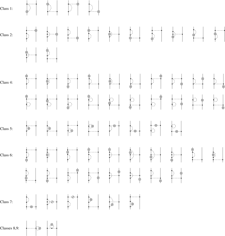
Figure 1: Leading loop contributions to the one-pion exchange current operator. Solid and dashed lines refer to nucleons and pions, respectively. Solid dots are the lowest-order vertices from the effective Lagrangian while the circle-crosses represent insertions of the electromagnetic vertices as explained in the text. Diagrams resulting from interchanging the nucleon lines are not shown.

Notice that while class-$3$ terms proportional to $g_{A}^{0}$ and involving an insertion of $J^{\mu}_{02}$ contribute to the two-pion exchange current, they do not generate one-pion exchange diagrams. On the other hand we now have additional contributions from class-$8,9$ terms which do not contribute to two-pion exchange diagrams and, for that reason, were not considered in Ref. Kolling:2009iq . We further emphasize that, strictly, speaking (i.e. according to the power of $g_{A}$), these diagrams belong to class 5. The algebraic structure of the current operator in Fock space in terms of $H_{ab}$ and $J^{\mu}_{ab}$ for seven classes is given in appendix A of Ref. Kolling:2009iq . The new terms corresponding to the classes 8 and 9 have the form:

$$J_{\rm c8} = \eta\left[H_{21}^{(1)}\frac{\lambda^{1}}{E_{\pi}}H_{23}^{(3)}\frac{\lambda^{2}}{E_{\pi}}J_{02}^{(-1)}+H_{21}^{(1)}\frac{\lambda^{1}}{E_{\pi}}J_{02}^{(-1)}\frac{\lambda^{3}}{E_{\pi}}H_{23}^{(3)}+H_{23}^{(3)}\frac{\lambda^{3}}{E_{\pi}}H_{21}^{(1)}\frac{\lambda^{2}}{E_{\pi}}J_{02}^{(-1)}\right]\eta+\textrm{h.c.}\,,$$

$$J_{\rm c9} = -\eta\biggl{[}H_{21}^{(1)}\frac{\lambda^{1}}{E_{\pi}}H_{21}^{(1)}\frac{\lambda^{2}}{E_{\pi}}H_{04}^{(2)}\frac{\lambda^{2}}{E_{\pi}}J_{02}^{(-1)}+H_{21}^{(1)}\frac{\lambda^{1}}{E_{\pi}}H_{04}^{(2)}\frac{\lambda^{3}}{E_{\pi}}H_{21}^{(1)}\frac{\lambda^{2}}{E_{\pi}}J_{02}^{(-1)}+H_{04}^{(2)}\frac{\lambda^{4}}{E_{\pi}}H_{21}^{(1)}\frac{\lambda^{3}}{E_{\pi}}H_{21}^{(1)}\frac{\lambda^{2}}{E_{\pi}}J_{02}^{(-1)}$$

$${}+H_{21}^{(1)}\frac{\lambda^{1}}{E_{\pi}}H_{21}^{(1)}\frac{\lambda^{2}}{E_{\pi}}J_{02}^{(-1)}\frac{\lambda^{4}}{E_{\pi}}H_{04}^{(2)}+H_{21}^{(1)}\frac{\lambda^{1}}{E_{\pi}}H_{04}^{(2)}\frac{\lambda^{3}}{E_{\pi}}J_{02}^{(-1)}\frac{\lambda^{1}}{E_{\pi}}H_{21}^{(1)}+H_{21}^{(1)}\frac{\lambda^{1}}{E_{\pi}}J_{02}^{(-1)}\frac{\lambda^{3}}{E_{\pi}}H_{21}^{(1)}\frac{\lambda^{4}}{E_{\pi}}H_{04}^{(2)}\biggr{]}\eta+\textrm{h.c.}\,.$$

Here, the superscript $i$ of $\lambda^{i}$ refers to the number of pions in the corresponding intermediate state. Further, $E_{\pi}$ denotes the total energy of pions in the corresponding state, $E_{\pi}=\sum_{i}\sqrt{\vec{l}_{i}\,^{2}+M_{\pi}^{2}}$, with $\vec{l}_{i}$ the corresponding pion momenta. We remind the reader that the representation for the power counting in terms of the canonical dimension $\kappa$ allows one to easily read off the chiral order associated to a given contribution by simply adding together the dimensions $\kappa$ of $H_{ab}^{(\kappa)}$ and ${J^{\mu}_{ab}}^{(\kappa)}$.

As already pointed out in section II and in Ref. Kolling:2009iq , we have to employ additional UTs in the $\eta$-space in order to maintain renormalizability of the one-pion exchange contributions, see Refs. Epelbaum:2007us for a related discussion. For the case at hand, one can distinguish between the strong UTs and the ones depending on the electromagnetic four-potential $\mathcal{A}$. The general form of the strong UTs up to the considered order in the chiral expansion is given in Ref. Epelbaum:2007us . These continuous UTs are parametrized in terms of some (a-priori arbitrary) “angles” $\bar{\alpha}_{i}$. These parameters turn out to be strongly constrained if one requires that matrix elements of the resulting nuclear potentials can be made finite by means of redefinition of certain LECs, i.e. if one demands renormalizability at the level of the nuclear Hamiltonian. For the UTs considered in Ref. Epelbaum:2007us , this condition was shown to lead to a unique expression for the four-nucleon force which does not depend on $\bar{\alpha}_{i}$ any more. Similarly, the expressions for the two-pion exchange current operator obtained in Ref. Kolling:2009iq are also $\bar{\alpha}_{i}$-independent. The additional electromagnetic UTs have not been discussed in that reference as they turned out not to affect the two-pion exchange contributions. As will be shown below, it is necessary to employ such additional UTs to maintain renormalizability of the one-pion exchange current. To be specific, we consider the $\eta$-space UT of the form

$$U=e^{S}$$ (4.2)

where $S$ is an anti-hermitian operator acting in the $\eta$-space, $S=\eta S\eta$, $S^{\dagger}=-S$. At the order considered, this operator can be parametrized as

$$S=\sum_{i=1}^{7}\bar{\beta}_{i}S_{i}$$ (4.3)

with $\bar{\beta}_{i}$ being arbitrary constants and

$$S_{1} = \eta\left[J_{02}^{(-1)}\frac{\lambda^{2}}{E_{\pi}^{2}}H_{22}^{(2)}\;-\;H_{22}^{(2)}\frac{\lambda^{2}}{E_{\pi}^{2}}J_{02}^{(-1)}\right]\eta\,,$$

$$S_{2} = \eta\left[H_{21}^{(1)}\frac{\lambda^{1}}{E_{\pi}^{2}}J_{20}^{(-1)}\frac{\lambda^{1}}{E_{\pi}}H_{21}^{(1)}\;-\;H_{21}^{(1)}\frac{\lambda^{1}}{E_{\pi}}J_{20}^{(-1)}\frac{\lambda^{1}}{E_{\pi}^{2}}H_{21}^{(1)}\right]\eta\,,$$

$$S_{3} = \eta\left[J_{20}^{(-1)}\eta H_{21}^{(1)}\frac{\lambda^{1}}{E_{\pi}^{3}}H_{21}^{(1)}\;-\;H_{21}^{(1)}\frac{\lambda^{1}}{E_{\pi}^{3}}H_{21}^{(1)}\eta J_{02}^{(-1)}\right]\eta\,,$$

$$S_{4} = \eta\left[J_{02}^{(-1)}\frac{\lambda^{2}}{E_{\pi}^{2}}H_{21}^{(1)}\frac{\lambda^{1}}{E_{\pi}}H_{21}^{(1)}-H_{21}^{(1)}\frac{\lambda^{1}}{E_{\pi}}H_{21}^{(1)}\frac{\lambda^{2}}{E_{\pi}^{2}}J_{02}^{(-1)}\right]\eta\,,$$

$$S_{5} = \eta\left[J_{02}^{(-1)}\frac{\lambda^{1}}{E_{\pi}}H_{21}^{(1)}\frac{\lambda^{1}}{E_{\pi}^{2}}H_{21}^{(1)}-H_{21}^{(1)}\frac{\lambda^{1}}{E_{\pi}^{2}}H_{21}^{(1)}\frac{\lambda^{2}}{E_{\pi}}J_{02}^{(-1)}\right]\eta\,,$$

$$S_{6} = \eta\left[H_{21}^{(1)}\frac{\lambda^{1}}{E_{\pi}}J_{02}^{(-1)}\frac{\lambda^{1}}{E_{\pi}^{2}}H_{21}^{(1)}-H_{21}^{(1)}\frac{\lambda^{1}}{E_{\pi}^{2}}J_{02}^{(-1)}\frac{\lambda^{2}}{E_{\pi}}H_{21}^{(1)}\right]\eta\,,$$

$$S_{7} = \eta\left[H_{21}^{(1)}\frac{\lambda^{1}}{E_{\pi}^{3}}J_{21}^{(0)}-J_{21}^{(0)}\frac{\lambda^{1}}{E_{\pi}^{3}}H_{21}^{(1)}\right]\eta\,.$$ (4.4)

The action of these UTs onto the one-pion exchange contribution to the lowest-order effective Hamilton operator,

$$H^{(0)}=\eta\left[H_{20}^{(2)}+H_{40}^{(2)}-H_{21}^{(1)}\frac{\lambda^{1}}{E_{\pi}}H_{21}^{(1)}\right]\,,$$ (4.5)

with $H_{20}^{(2)}$ denoting the nonrelativistic kinetic energy term, induces additional, $\bar{\beta}$-dependent class-2, class-5, class-6 and class-7 contributions:

$$\delta J_{\rm c2} = \beta_{7}\,\eta\left[H_{21}^{(1)}\frac{\lambda^{1}}{E_{\pi}}H_{21}^{(1)}\eta H_{21}^{(1)}\frac{\lambda^{1}}{E_{\pi}^{3}}J_{21}^{(0)}-H_{21}^{(1)}\frac{\lambda^{1}}{E_{\pi}}H_{21}^{(1)}\eta J_{21}^{(0)}\frac{\lambda^{1}}{E_{\pi}^{3}}H_{21}^{(1)}\right]\eta+\textrm{h.c.}\,,$$

$$\delta J_{\rm c5} = \bar{\beta}_{1}\,\eta\left[H_{21}^{(1)}\frac{\lambda^{1}}{E_{\pi}}H_{21}^{(1)}\eta J_{02}^{(-1)}\frac{\lambda^{2}}{E_{\pi}^{2}}H_{22}^{(2)}-H_{21}^{(1)}\frac{\lambda^{1}}{E_{\pi}}H_{21}^{(1)}\eta H_{22}^{(2)}\frac{\lambda^{2}}{E_{\pi}^{2}}J_{02}^{(-1)}\right]\eta+\textrm{h.c.}\,,$$

$$\delta J_{\rm c6} = \bar{\beta}_{2}\,\eta\left[H_{21}^{(1)}\frac{\lambda^{1}}{E_{\pi}}H_{21}^{(1)}\eta H_{21}^{(1)}\frac{\lambda^{1}}{E_{\pi}^{2}}J_{20}^{(-1)}\frac{\lambda^{1}}{E_{\pi}}H_{21}^{(1)}-H_{21}^{(1)}\frac{\lambda^{1}}{E_{\pi}^{2}}J_{20}^{(-1)}\frac{\lambda^{1}}{E_{\pi}}H_{21}^{(1)}\eta H_{21}^{(1)}\frac{\lambda^{1}}{E_{\pi}}H_{21}^{(1)}\right]\eta+\textrm{h.c.}\,,$$

$$+ \bar{\beta}_{3}\,\eta\left[H_{21}^{(1)}\frac{\lambda^{1}}{E_{\pi}^{3}}H_{21}^{(1)}\eta J_{20}^{(-1)}\eta H_{21}^{(1)}\frac{\lambda^{1}}{E_{\pi}}H_{21}^{(1)}-\eta H_{21}^{(1)}\frac{\lambda^{1}}{E_{\pi}}H_{21}^{(1)}\eta H_{21}^{(1)}\frac{\lambda^{1}}{E_{\pi}^{3}}H_{21}^{(1)}\eta J_{20}^{(-1)}\right]\eta+\textrm{h.c.}\,,$$

$$\delta J_{\rm c7} = \bar{\beta}_{4}\,\eta\biggl{[}H_{21}^{(1)}\frac{\lambda^{1}}{E_{\pi}}H_{21}^{(1)}\eta J_{(02)}^{(-1)}\frac{\lambda^{2}}{E_{\pi}^{2}}H_{21}^{(1)}\frac{\lambda^{1}}{E_{\pi}}H_{21}^{(1)}-H_{21}^{(1)}\frac{\lambda^{1}}{E_{\pi}}H_{21}^{(1)}\eta H_{21}^{(1)}\frac{\lambda^{1}}{E_{\pi}}H_{21}^{(1)}\frac{\lambda^{2}}{E_{\pi}^{2}}J_{02}^{(-1)}\biggr{]}\eta+\textrm{h.c.}\,,$$ (4.6)

$$+ \bar{\beta}_{5}\,\eta\biggl{[}H_{21}^{(1)}\frac{\lambda^{1}}{E_{\pi}}H_{21}^{(1)}\eta J_{02}^{(-1)}\frac{\lambda^{2}}{E_{\pi}}H_{\pi N}\frac{\lambda^{1}}{E_{\pi}^{2}}H_{21}^{(1)}-H_{21}^{(1)}\frac{\lambda^{1}}{E_{\pi}}H_{21}^{(1)}\eta H_{21}^{(1)}\frac{\lambda^{1}}{E_{\pi}^{2}}H_{21}^{(1)}\frac{\lambda^{2}}{E_{\pi}}J_{02}^{(-1)}\biggr{]}\eta+\textrm{h.c.}\,,$$

$$+ \bar{\beta}_{6}\,\eta\biggl{[}H_{21}^{(1)}\frac{\lambda^{1}}{E_{\pi}}H_{21}^{(1)}\eta H_{21}^{(1)}\frac{\lambda^{1}}{E_{\pi}^{2}}J_{02}^{(-1)}\frac{\lambda^{1}}{E_{\pi}}H_{21}^{(1)}-H_{21}^{(1)}\frac{\lambda^{1}}{E_{\pi}}H_{21}^{(1)}\eta H_{21}^{(1)}\frac{\lambda^{1}}{E_{\pi}}J_{02}^{(-1)}\frac{\lambda^{1}}{E_{\pi}^{2}}H_{21}^{(1)}\biggr{]}\eta+\textrm{h.c.}\,.$$

It turns out to be convenient to express $\bar{\beta}_{4,5,6}$ in terms of another set of constants $\beta$, $\gamma$ and $\delta$ defined as:

$$\bar{\beta}_{4}\equiv-\beta+\delta\,,\qquad 2\bar{\beta}_{5}\equiv-\beta+\gamma\,,\qquad 2\bar{\beta}_{6}\equiv-\beta-\gamma\,.$$ (4.7)

Already at this stage we emphasize that three of the seven parameters, namely $\gamma$, $\bar{\beta}_{2}$ and $\bar{\beta}_{7}$, do not affect the leading one-loop contributions to the one-pion exchange matrix elements.

After these preliminary remarks, we are now in the position to discuss the results for the one-loop contributions. Here and in what follows, the expressions for a class-$X$ contribution $J_{\rm cX}^{\mu}$ refer to the matrix element defined according to

$$\langle\vec{p}_{1}{}^{\prime}\,\vec{p}_{2}{}^{\prime}|J^{\mu}|\vec{p}_{1}\,\vec{p}_{2}\rangle=\delta(\vec{p}_{1}{}^{\prime}+\vec{p}_{2}{}^{\prime}-\vec{p}_{1}-\vec{p}_{2}-\vec{k})\,\left[J_{\rm cX}^{\mu}\,+\,(1\leftrightarrow 2)\right]\,.$$ (4.8)

Here and in what follows, $\vec{p}_{i}$ ($\vec{p}_{i}\,^{\prime}$) refers to the initial (final) momentum of the nucleon $i$. We will also frequently use the momentum transfer variables $q_{1,2}\equiv\vec{p}_{1,2}\,^{\prime}-\vec{p}_{1,2}$. The expressions for the two-pion exchange current and charge densities were given in Ref. Kolling:2009iq in terms of the most general set of spin-momentum vector and scalar operators $\vec{O}_{1\ldots 24}$ and $O_{1\ldots 8}^{S}$ as well as isospin operators $T_{1\ldots 5}$. We found that this representation leads to unnecessarily involved expressions in the case of the one-pion exchange and short-range currents. We, therefore, refrain from using the operators $\vec{O}_{1\ldots 24}$, $O_{1\ldots 8}^{S}$ and $T_{1\ldots 5}$ in the present work.

Evaluating matrix elements of the operators in the Fock space as discussed above, we obtain the following results for the matrix elements of the current density:

$$\vec{J}_{\rm c1} = -e\frac{\mathring{g}_{A}^{2}i}{16F^{4}}\left[\vec{\tau}_{1}\times\vec{\tau}_{2}\right]^{3}\,\vec{\sigma}_{1}\frac{\vec{\sigma}_{2}\cdot\vec{q}_{2}}{q_{2}^{2}+M_{\pi}^{2}}\int\frac{d^{3}l}{(2\pi)^{3}}\frac{1}{\omega_{l}}\,,$$

$$\vec{J}_{\rm c2} = e\frac{\mathring{g}_{A}^{4}i}{6F^{4}}\left[\vec{\tau}_{1}\times\vec{\tau}_{2}\right]^{3}\,\vec{\sigma}_{1}\frac{\vec{\sigma}_{2}\cdot\vec{q}_{2}}{q_{2}^{2}+M_{\pi}^{2}}\int\frac{d^{3}l}{(2\pi)^{3}}\frac{l^{2}}{\omega_{l}^{3}}\,,$$

$$\vec{J}_{\rm c5} = e\frac{\mathring{g}_{A}^{2}\,i}{32F^{4}}\left[\vec{\tau}_{1}\times\vec{\tau}_{2}\right]^{3}\,\frac{\vec{\sigma}_{2}\cdot\vec{q}_{2}}{q_{2}^{2}+M_{\pi}^{2}}\,\int\frac{d^{3}l}{(2\pi)^{3}}\vec{l}\,\frac{\vec{l}\cdot\vec{\sigma}_{1}}{\omega_{+}\omega_{-}(\omega_{+}+\omega_{-})}$$

$${}-\left(1-\bar{\beta}_{1}\right)e\frac{\mathring{g}_{A}^{2}\,i}{16F^{4}}\left[\vec{\tau}_{1}\times\vec{\tau}_{2}\right]^{3}\frac{\vec{\sigma}_{2}\cdot\vec{q}_{2}}{q_{2}^{2}+M_{\pi}^{2}}\,\vec{\sigma}_{1}\cdot\vec{q}_{1}\int\frac{d^{3}l}{(2\pi)^{3}}\,\vec{l}\,\frac{\omega_{-}-\omega_{+}}{\omega_{+}\omega_{-}(\omega_{+}+\omega_{-})^{2}}\,,$$

$$\vec{J}_{\rm c7} = -e\frac{\mathring{g}_{A}^{4}i}{4F^{4}}\,\left[\vec{\tau}_{1}\times\vec{\tau}_{2}\right]^{3}\left(\vec{q}_{1}-\vec{q}_{2}\right)\frac{\vec{\sigma}_{1}\cdot\vec{q}_{1}}{q_{1}^{2}+M_{\pi}^{2}}\frac{\vec{\sigma}_{2}\cdot\vec{q}_{2}}{q_{2}^{2}+M_{\pi}^{2}}\,\frac{1}{3}\int\frac{d^{3}l}{(2\pi)^{3}}\frac{l^{2}}{\omega_{l}^{3}}\,$$

$${}+e\frac{\mathring{g}_{A}^{4}i}{8F^{4}}\left[\vec{\tau}_{1}\times\vec{\tau}_{2}\right]^{3}\frac{\vec{\sigma}_{2}\cdot\vec{q}_{2}}{q_{2}^{2}+M_{\pi}^{2}}\,\int\frac{d^{3}l}{(2\pi)^{3}}\,\vec{l}\,\left(\vec{l}\cdot\vec{q}_{2}\vec{\sigma}_{1}\cdot\vec{k}-\vec{k}\cdot\vec{q}_{2}\vec{\sigma}_{1}\cdot\vec{l}\right)\frac{\omega_{+}^{2}+\omega_{+}\omega_{-}+\omega_{-}^{2}}{\omega_{+}^{3}\omega_{-}^{3}(\omega_{+}+\omega_{-})}$$

$${}-e\frac{\mathring{g}_{A}^{4}i}{32F^{4}}\left[\vec{\tau}_{1}\times\vec{\tau}_{2}\right]^{3}\frac{\vec{\sigma}_{2}\cdot\vec{q}_{2}}{q_{2}^{2}+M_{\pi}^{2}}\,\vec{\sigma}_{1}\cdot\vec{q}_{2}\,\int\frac{d^{3}l}{(2\pi)^{3}}\,\vec{l}\,(k^{2}-l^{2})\,\biggl{[}2(\beta-1)\frac{(\omega_{-}-\omega_{+})(\omega_{+}^{2}+3\omega_{+}\omega_{-}+\omega_{-}^{2})}{\omega_{+}^{3}\omega_{-}^{3}(\omega_{+}+\omega_{-})^{2}}$$

$${}+\delta\frac{(\omega_{-}-\omega_{+})(\omega_{-}^{2}+\omega_{+}^{2})}{\omega_{-}^{3}\omega_{+}^{3}(\omega_{+}+\omega_{-})^{2}}\biggr{]}\,,$$

$$\vec{J}_{\rm c8} = -e\frac{\mathring{g}_{A}^{2}\,i}{32F^{4}}\left[\vec{\tau}_{1}\times\vec{\tau}_{2}\right]^{3}\frac{\vec{\sigma}_{2}\cdot\vec{q}_{2}}{q_{2}^{2}+M_{\pi}^{2}}\int\frac{d^{3}l}{(2\pi)^{3}}\vec{l}\ \frac{\vec{l}\cdot\vec{\sigma}_{1}}{\omega_{+}\omega_{-}(\omega_{+}+\omega_{-})}\,,$$

$$\vec{J}_{\rm c9} = e\frac{\mathring{g}_{A}^{2}\,i}{32F^{4}}\left[\vec{\tau}_{1}\times\vec{\tau}_{2}\right]^{3}\frac{\vec{\sigma}_{1}\cdot\vec{q}_{1}}{q_{1}^{2}+M_{\pi}^{2}}\frac{\vec{\sigma}_{1}\cdot\vec{q}_{2}}{q_{2}^{2}+M_{\pi}^{2}}\int\frac{d^{3}l}{(2\pi)^{3}}\vec{l}\ \frac{\vec{l}\cdot\left(\vec{q}_{1}-\vec{q}_{2}\right)}{\omega_{+}\omega_{-}(\omega_{+}+\omega_{-})}\,,$$ (4.9)

and the charge density:

$$\rho_{\rm c6} = e\frac{\mathring{g}_{A}^{4}}{4F^{4}}\,\frac{1}{3}\,\tau_{2}^{3}\,\vec{\sigma}_{1}\cdot\vec{q}_{2}\,\frac{\vec{\sigma}_{2}\cdot\vec{q}_{2}}{q_{2}^{2}+M_{\pi}^{2}}\,\int\frac{d^{3}l}{(2\pi)^{3}}\frac{l^{2}}{\omega_{l}^{4}}\,,$$

$$\rho_{\rm c7} = -e\frac{\mathring{g}_{A}^{4}}{8F^{4}}\ \tau_{2}^{3}\,\frac{\vec{\sigma}_{2}\cdot\vec{q}_{2}}{q_{2}^{2}+M_{\pi}^{2}}\int\frac{d^{3}l}{(2\pi)^{3}}\left(\vec{\sigma}_{1}\cdot\vec{l}\,\vec{q}_{2}\cdot\vec{l}-\vec{\sigma}_{1}\cdot\vec{k}\,\vec{q}_{2}\cdot\vec{k}\right)\frac{1}{\omega_{+}^{2}\omega_{-}^{2}}\,,$$ (4.10)

where

$$\omega_{\pm}^{2}=\left(\vec{l}\pm\vec{k}\right)^{2}+4M_{\pi}^{2}\,,\quad\quad\omega_{l}^{2}=\vec{l}\,^{2}+M_{\pi}^{2}\,.$$ (4.11)

The class-$3,4,6$ contributions to the current density and class-$1,2,3,4,5,8,9$ contributions to the charge density are found to vanish.

IV.2 Tree level contributions

The loop contributions considered in the previous section do not involve the ones emerging from pion tadpole diagrams. These must be explicitly taken into account if one wants to use the values of the renormalized LECs such as $d_{i}$ determined from e.g. the pion-nucleon system. The treatment of the pion tadpoles in the method of unitary transformation is discussed in detail in Ref. Epelbaum:2002gb . The pion tadpole contributions emerge from contractions of the pion field operators when performing the normal ordering of the effective pion-nucleon Hamiltonian and simply lead to additional vertex corrections. Following Ref. Epelbaum:2002gb , we work with renormalized pion field and mass defined according to

$$\pi_{a}^{r}=Z_{\pi}^{-1/2}\pi_{a}\,,\quad\quad Z_{\pi}=1+\delta Z_{\pi}\,,\quad\quad M_{\pi}^{2}=M^{2}+\delta M_{\pi}^{2}\,,$$ (4.12)

where $a$ denotes the isospin quantum number and $\delta Z_{\pi},\;\delta M_{\pi}^{2}/M_{\pi}^{2}\sim\mathcal{O}(Q^{2}/\Lambda^{2})$. At the leading loop order, $\delta Z_{\pi}$ and $\delta M_{\pi}^{2}$ are given by Epelbaum:2002gb

$$\delta Z_{\pi} = -\frac{2l_{4}M_{\pi}^{2}}{F^{2}}-\frac{1-10\xi}{F^{2}}\Delta_{\pi}\,,$$

$$M_{\pi}^{2} = M^{2}\left(1+\frac{2l_{3}M_{\pi}^{2}}{F^{2}}+\frac{1-8\xi}{2F^{2}}\Delta_{\pi}\right)\,,$$

where the quantity $\Delta_{\pi}$ is defined in Eq. (B.5). Notice that in Ref. Epelbaum:2002gb we used the parametrization of the matrix $U$ with $\xi=0$. We further emphasize that there are no pion self-energy diagrams since we work with renormalized pion fields. All effects due to pion self-energy and/or tadpoles are taken into account by vertex corrections in the normal-ordered effective Hamiltonian. This is schematically visualized in Fig. 2. More precisely, replacing $\pi_{a}\to\pi_{a}^{r}$ and $M^{2}\to M_{\pi}^{2}$ in $\mathcal{L}_{\pi\pi}^{(2)}$ and $\mathcal{L}_{\pi N}^{(1)}$ generates corrections to $\mathcal{L}_{\pi\pi}^{(4)}$ and $\mathcal{L}_{\pi N}^{(3)}$ (and, of course, in the corresponding Hamilton densities) driven by $\delta Z_{\pi}$ and $\delta M_{\pi}^{2}$. Further corrections, $\delta_{\rm NO}$, to the operators $H_{21}^{(3)}$, $J_{21}^{(2)}$ and $J_{02}^{(1)}$ emerge from taking normal ordering on the operators $H_{23}^{(3)}$, $J_{23}^{(3)}$ and $J_{04}^{(1)}$ Together with the the wave function renormalization of the pion, we obtain the following shifts:

$$H_{21}^{(3)} \rightarrow H_{21}^{(3)}+H_{21}^{(1)}\left(\frac{1}{2}\delta Z_{\pi}+\delta_{\rm NO}\right)=H_{21}^{(3)}-\,H_{21}^{(1)}\frac{l_{4}M_{\pi}^{2}}{F^{2}}\,,$$

$${\vec{J}_{21}\,}^{\,(2)} \rightarrow {\vec{J}_{21}\,}^{\,(2)}+{\vec{J}_{21}\,}^{\,(0)}\left(\frac{1}{2}\delta Z_{\pi}+\delta_{\rm NO}\right)={\vec{J}_{21}\,}^{\,(2)}-{\vec{J}_{21}\,}^{\,(0)}\left(\frac{l_{4}M_{\pi}^{2}}{F^{2}}+\frac{1}{2F^{2}}\Delta_{\pi}\right)\,,$$

$${\vec{J}_{02}\,}^{\,(1)} \rightarrow {\vec{J}_{02}\,}^{\,(1)}+{\vec{J}_{02}\,}^{\,(-1)}\left(\delta Z_{\pi}+\delta_{\rm NO}\right)={\vec{J}_{02}\,}^{\,(1)}-{\vec{J}_{02}\,}^{\,(-1)}\left(\frac{2l_{4}M_{\pi}^{2}}{F^{2}}+\frac{1}{F^{2}}\Delta_{\pi}\right)\,.$$ (4.13)

We point out that, as expected, none of the renormalized operators depends on the (arbitrary) value of $\xi$.

\psfrag{plus}{\ $+$}\psfrag{arrow}{\ $\rightarrow$}\includegraphics[width=372.91345pt,keepaspectratio,angle={0},clip]{renormalization2.eps}

Figure 2: Schematic representation of the renormalization of the pion field and the operators $H_{21}^{(3)}$, $J_{21}^{(2)}$ and $J_{02}^{(1)}$

After these preliminary remarks, we are now in the position to discuss the tree-level contributions to the one-pion exchange current and charge densities. The formal operator structure is given by

$$J_{\rm tree} = \eta\biggr{[}-H_{21}^{(3)}\frac{\lambda^{1}}{E_{\pi}}J_{21}^{(0)}+H_{21}^{(3)}\frac{\lambda^{1}}{E_{\pi}}J_{20}^{(-1)}\frac{\lambda^{1}}{E_{\pi}}H_{21}^{(1)}-\frac{1}{2}J_{20}^{(-1)}\eta H_{21}^{(1)}\frac{\lambda^{1}}{E_{\pi}^{2}}H_{21}^{(3)}-\frac{1}{2}J_{20}^{(-1)}\eta H_{21}^{(3)}\frac{\lambda^{1}}{E_{\pi}^{2}}H_{21}^{(1)}$$ (4.14)

$${}+H_{21}^{(1)}\frac{\lambda^{1}}{E_{\pi}^{2}}H_{21}^{(3)}\eta J_{20}^{(-1)}-H_{21}^{(3)}\frac{\lambda^{1}}{E_{\pi}^{2}}H_{21}^{(1)}\eta J_{20}^{(-1)}+H_{21}^{(3)}\frac{\lambda^{1}}{E_{\pi}}J_{02}^{(-1)}\frac{\lambda^{1}}{E_{\pi}}H_{21}^{(1)}+J_{02}^{(-1)}\frac{\lambda^{2}}{E_{\pi}}H_{21}^{(1)}\frac{\lambda^{1}}{E_{\pi}}H_{21}^{(3)}$$

$${}+J_{02}^{(-1)}\frac{\lambda^{2}}{E_{\pi}}H_{21}^{(3)}\frac{\lambda^{1}}{E_{\pi}}H_{21}^{(1)}+H_{21}^{(1)}\frac{\lambda^{1}}{E_{\pi}}J_{20}^{(1)}\frac{\lambda^{1}}{E_{\pi}}H_{21}^{(1)}-H_{21}^{(1)}\frac{\lambda^{1}}{E_{\pi}^{2}}H_{21}^{(1)}\eta J_{20}^{(1)}-H_{21}^{(1)}\frac{\lambda^{1}}{E_{\pi}}J_{21}^{(2)}+H_{21}^{(1)}\frac{\lambda^{1}}{E_{\pi}}H_{21}^{(1)}\frac{\lambda^{2}}{E_{\pi}}J_{20}^{(1)}$$

$${}+\frac{1}{2}H_{21}^{(1)}\frac{\lambda^{1}}{E_{\pi}}J_{20}^{(1)}\frac{\lambda^{1}}{E_{\pi}}H_{21}^{(1)}\biggl{]}\eta+\textrm{h.c.}\,.$$

These operators give rise to diagrams shown in Fig. 3.

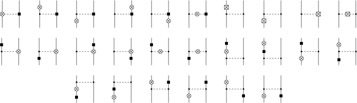
Figure 3: Contributions of the counter terms. Solid dots are the lowest-order vertices from the effective Lagrangian while the crosses represent insertions of the electromagnetic vertices as explained in the text. For remaining notation see Fig. 1.

The explicit form of all vertices entering this expression can be found in appendix A. Evaluating the corresponding matrix elements we obtain the following expressions for the current density

$$\vec{J}_{\rm tree} = 2e\frac{\mathring{g}_{A}\,i}{F^{2}}\left(d_{8}\tau_{2}^{3}+d_{9}\left(\vec{\tau}_{1}\cdot\vec{\tau}_{2}\right)\right)\frac{\vec{\sigma}_{2}\cdot\vec{q}_{2}}{q_{2}^{2}+M_{\pi}^{2}}\left[\vec{q}_{1}\times\vec{q}_{2}\right]-e\,\frac{\mathring{g}_{A}\,i}{4F^{2}}\left[\vec{\tau}_{1}\times\vec{\tau}_{2}\right]^{3}\,\frac{\vec{\sigma}_{2}\cdot\vec{q}_{2}}{q_{2}^{2}+M_{\pi}^{2}}\,\biggl{\{}2d_{21}\,\vec{k}\times\left[\vec{q}_{2}\times\vec{\sigma}_{1}\right]$$ (4.15)

$${}+d_{22}\,\vec{k}\times\left[\vec{q}_{1}\times\vec{\sigma}_{1}\right]+\vec{\sigma}_{1}\,\left[2M_{\pi}^{2}\,\left(4d_{16}-2d_{18}-\frac{l_{4}\mathring{g}_{A}}{F^{2}}\right)-\frac{\mathring{g}_{A}}{2}\Delta_{\pi}\right]$$

$${}-\vec{q}_{1}\frac{\vec{\sigma}_{1}\cdot\vec{q}_{1}}{q_{1}^{2}+M_{\pi}^{2}}\left[2M_{\pi}^{2}\,\left(4d_{16}-2d_{18}-\frac{l_{4}\mathring{g}_{A}}{F^{2}}\right)-\mathring{g}_{A}\Delta_{\pi}+\mathring{g}_{A}\,k^{2}\frac{l_{6}}{F^{2}}-\mathring{g}_{A}\,\frac{l_{6}}{F^{2}}\left(q_{1}^{2}-q_{2}^{2}\right)\right]\biggl{\}}\,,$$

while the contributions to the charge density vanish. This is consistent with the fact that the loop contributions to the charge density do not contain logarithmic ultraviolet divergences.

IV.3 Renormalization

The expressions given in the previous sections are written in terms of bare parameters and contain ultraviolet-divergent pieces. These divergences are cancelled after expressing the bare parameters $M$, $\mathring{g}_{A}$, $F$, $l_{i}$ and $d_{i}$ in terms of the corresponding renormalized quantities. When carrying out renormalization, one should also take into account the contribution induced by the leading-order ($\mathcal{O}\left(eQ^{-1}\right)$) one-pion exchange current shown in Fig. 4

$$\vec{J}^{\;\left(eQ^{-1}\right)}_{1\pi}=e\,\frac{i\mathring{g}_{A}^{2}}{4F^{2}}\left[\vec{\tau}_{1}\times\vec{\tau}_{2}\right]^{3}\,\frac{\vec{\sigma}_{2}\cdot\vec{q}_{2}}{q_{2}^{2}+M_{\pi}^{2}}\,\left(\vec{q}_{1}\frac{\vec{\sigma}_{1}\cdot\vec{q}_{1}}{q_{1}^{2}+M_{\pi}^{2}}-\vec{\sigma}_{1}\,\right)\,,$$ (4.16)

when expressing the ratio $\mathring{g}_{A}/F$ in terms of the physical LECs $g_{A}/F_{\pi}$.

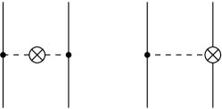
Figure 4: Lowest-order contributions to the pion exchange current operator: the pion-in-flight and seagull graphs. For notation see Fig. 1.

The chiral expansion of this ratio has the form

$$\frac{g_{A}}{F_{\pi}}=\frac{\mathring{g}_{A}}{F}\left(1-\frac{2g_{A}^{2}}{F_{\pi}^{2}}\Delta_{\pi}-\frac{M_{\pi}^{2}}{F_{\pi}^{2}}l_{4}+4\frac{M_{\pi}^{2}}{g_{A}}d_{16}\ \right)\,,$$ (4.17)

Clearly, this relation holds modulo higher-order corrections. The resulting induced correction at order $\mathcal{O}\left(eQ\right)$ reads:

$$\vec{J}^{\;\left(eQ\right)}_{1\pi}=e\frac{g_{A}^{2}\,i}{2F_{\pi}^{2}}\,\frac{\vec{\sigma}_{2}\cdot\vec{q}_{2}}{q_{2}^{2}+M_{\pi}^{2}}\,\left[\vec{\tau}_{1}\times\vec{\tau}_{2}\right]^{3}\,\left[\vec{q}_{1}\frac{\vec{\sigma}_{1}\cdot\vec{q}_{1}}{q_{1}^{2}+M_{\pi}^{2}}-\vec{\sigma}_{1}\right]\left(\frac{2g_{A}^{2}}{F_{\pi}^{2}}\Delta_{\pi}+\frac{M_{\pi}^{2}}{F_{\pi}^{2}}l_{4}-4\frac{M_{\pi}^{2}}{g_{A}}d_{16}\right)\,.$$ (4.18)

Notice that at the order considered, one can safely replace $\mathring{g}_{A}$ and $F$ by the corresponding renormalized quantities in all expressions given in sections IV.1 and IV.2.

Consider now the LECs $l_{i}$ and $d_{i}$ which can be decomposed into the divergent parts and finite pieces as follows:

$$l_{i} = l_{i}^{r}(\mu)+\gamma_{i}L=\frac{1}{16\pi^{2}}\bar{l}_{i}+\gamma_{i}L+\gamma_{i}\frac{1}{16\pi^{2}}\log\left(\frac{M_{\pi}}{\mu}\right)\,,$$

$$d_{i} = d_{i}^{r}(\mu)+\frac{\beta_{i}}{F^{2}}L=\bar{d}_{i}+\frac{\beta_{i}}{F^{2}}L+\frac{\beta_{i}}{16\pi^{2}F^{2}}\log\left(\frac{M_{\pi}}{\mu}\right)\,,$$ (4.19)

where the divergent quantity $L$ is defined in Eq. (B.6). The corresponding coefficients $\beta_{i}$ and $\gamma_{i}$ in the framework of dimensional regularization (DR) are well known Gasser:1983yg ; Ecker:1995rk ; Fettes:1998ud ; Gasser:2002am and read:

$$\beta_{8}=\beta_{9}=\beta_{18}=\beta_{22}=0,\quad\quad\beta_{16}=\frac{1}{2}g_{A}+g_{A}^{3},\quad\quad\beta_{21}=-g_{A}^{3},\quad\quad\gamma_{4}=2,\quad\quad\gamma_{6}=-\frac{1}{3}\,.$$ (4.20)

The expressions for all loop integrals that enter the calculation in DR can be found in Appendix B. The only exception is the part of the class-7 current proportional to the constant $\delta$, for which we did not succeed to find a closed expression. Inserting the DR expressions for the integrals entering Eqs. (IV.1), (IV.1) and the pion tadpole contributions discussed above and replacing the bare LECs in terms of renormalized ones, one observes that indeed almost all divergences cancel. The only remaining divergent part of the current reads

$$\vec{J}_{\rm div} = -e\frac{g_{A}^{2}\,i}{12F_{\pi}^{4}}\left[\vec{\tau}_{1}\times\vec{\tau}_{2}\right]^{3}\frac{\vec{\sigma}_{2}\cdot\vec{q}_{2}}{q_{2}^{2}+M_{\pi}^{2}}\,\vec{k}\ L\ \left[\vec{\sigma}_{1}\cdot\vec{q}_{1}\,\left(1-\bar{\beta}_{1}\right)\,+g_{A}^{2}\ \vec{\sigma}_{1}\cdot\vec{q}_{2}\left(-2+2\beta+\delta\right)\right]\,.$$ (4.21)

This implies that we have to choose $\bar{\beta}_{1}=1$ and $-2+2\beta+\delta=0$ in order to be able to renormalize the current operator. Here and in what follows, we adopt the choice $\delta=0$ and $\beta=1$.

IV.4 Relativistic corrections

Last but not least, we now discuss the leading relativistic corrections. These emerge from the operators in Eq. (4.14) with the vertices $H_{21}^{(3)}$, $J_{20}^{(1)}$ and $J_{21}^{(2)}$ being replaced by the corresponding relativistic corrections $\tilde{H}_{21}^{(3)}$, $\tilde{J}_{20}^{(1)}$ and $\tilde{J}_{21}^{(2)}$, respectively, whose explicit form is given in appendix A. In addition, there are contributions emerging from insertions of the kinetic energy of the nucleon $\tilde{H}_{20}^{(2)}$ which have the form

$$J_{1/m_{N}} = \eta\,\biggr{[}H_{21}^{(1)}\frac{\lambda^{1}}{E_{\pi}}\tilde{H}_{20}^{(2)}\frac{\lambda^{1}}{E_{\pi}}J_{21}^{(0)}-\tilde{H}_{20}^{(2)}\eta H_{21}^{(1)}\frac{\lambda^{1}}{E_{\pi}^{2}}J_{21}^{(0)}+\bar{\beta}_{7}\,\left(H_{21}^{(1)}\frac{\lambda^{1}}{E_{\pi}^{3}}J_{21}^{(0)}\eta\tilde{H}_{20}^{(2)}-\tilde{H}_{20}^{(2)}\eta H_{21}^{(1)}\frac{\lambda^{1}}{E_{\pi}^{3}}J_{21}^{(0)}\right)\,,$$ (4.22)

$$+ H_{21}^{(1)}\frac{\lambda^{1}}{E_{\pi}}J_{02}^{(-1)}\frac{\lambda^{1}}{E_{\pi}^{2}}H_{21}^{(1)}\eta\tilde{H}_{20}^{(2)}-H_{21}^{(1)}\frac{\lambda^{1}}{E_{\pi}}H_{21}^{(1)}\frac{\lambda^{2}}{E_{\pi}}\tilde{H}_{20}^{(2)}\frac{\lambda^{2}}{E_{\pi}}J_{02}^{(-1)}-H_{21}^{(1)}\frac{\lambda^{1}}{E_{\pi}}\tilde{H}_{20}^{(2)}\frac{\lambda^{1}}{E_{\pi}}H_{21}^{(1)}\frac{\lambda^{2}}{E_{\pi}}J_{02}^{(-1)}$$

$$- H_{21}^{(1)}\frac{\lambda^{1}}{E_{\pi}}\tilde{H}_{20}^{(2)}\frac{\lambda^{1}}{E_{\pi}}J_{02}^{(-1)}\frac{\lambda^{1}}{E_{\pi}}H_{21}^{(1)}+\tilde{H}_{20}^{(2)}\eta H_{21}^{(1)}\frac{\lambda^{1}}{E_{\pi}^{2}}H_{21}^{(1)}\frac{\lambda^{2}}{E_{\pi}}J_{02}^{(-1)}+\tilde{H}_{20}^{(2)}\eta H_{21}^{(1)}\frac{\lambda^{1}}{E_{\pi}}H_{21}^{(1)}\frac{\lambda^{2}}{E_{\pi}^{2}}J_{02}^{(-1)}$$

$$+ \bar{\beta}_{4}\,\biggr{(}\tilde{H}_{20}^{(2)}\eta H_{21}^{(1)}\frac{\lambda^{1}}{E_{\pi}}H_{21}^{(1)}\frac{\lambda^{2}}{E_{\pi}^{2}}J_{02}^{(-1)}-\tilde{H}_{20}^{(2)}\eta J_{02}^{(-1)}\frac{\lambda^{2}}{E_{\pi}^{2}}H_{21}^{(1)}\frac{\lambda^{1}}{E_{\pi}}H_{21}^{(1)}\biggl{)}+\bar{\beta}_{5}\,\biggr{(}\tilde{H}_{20}^{(2)}\eta H_{21}^{(1)}\frac{\lambda^{1}}{E_{\pi}^{2}}H_{21}^{(1)}\frac{\lambda^{2}}{E_{\pi}}J_{02}^{(-1)}$$

$$- \tilde{H}_{20}^{(2)}\eta J_{02}^{(-1)}\frac{\lambda^{2}}{E_{\pi}}H_{21}^{(1)}\frac{\lambda^{1}}{E_{\pi}^{2}}H_{21}^{(1)}\biggl{)}+\bar{\beta}_{6}\,\biggr{(}H_{21}^{(1)}\frac{\lambda^{1}}{E_{\pi}}J_{02}^{(-1)}\frac{\lambda^{1}}{E_{\pi}^{2}}H_{21}^{(1)}\eta\tilde{H}_{20}^{(2)}-H_{21}^{(1)}\frac{\lambda^{1}}{E_{\pi}^{2}}J_{02}^{(-1)}\frac{\lambda^{1}}{E_{\pi}}H_{21}^{(1)}\eta\tilde{H}_{20}^{(2)}\biggl{)}$$

$$+ H_{21}^{(1)}\frac{\lambda^{1}}{E_{\pi}}J_{20}^{(-1)}\frac{\lambda^{1}}{E_{\pi}^{2}}H_{21}^{(1)}\eta\tilde{H}_{20}^{(2)}-H_{21}^{(1)}\frac{\lambda^{1}}{E_{\pi}}\tilde{H}_{20}^{(2)}\frac{\lambda^{1}}{E_{\pi}}J_{20}^{(-1)}\frac{\lambda^{1}}{E_{\pi}}H_{21}^{(1)}-\frac{1}{2}H_{21}^{(1)}\frac{\lambda^{1}}{E_{\pi}^{3}}H_{21}^{(1)}\eta\tilde{H}_{20}^{(2)}\eta J_{20}^{(-1)}$$

$$+ \frac{1}{2}H_{21}^{(1)}\frac{\lambda^{1}}{E_{\pi}^{2}}\tilde{H}_{20}^{(2)}\frac{\lambda^{1}}{E_{\pi}}H_{21}^{(1)}\eta J_{20}^{(-1)}+\frac{1}{2}H_{21}^{(1)}\frac{\lambda^{1}}{E_{\pi}}\tilde{H}_{20}^{(2)}\frac{\lambda^{1}}{E_{\pi}^{2}}H_{21}^{(1)}\eta J_{20}^{(-1)}-\frac{1}{2}\tilde{H}_{20}^{(2)}\eta H_{21}^{(1)}\frac{\lambda^{1}}{E_{\pi}^{3}}H_{21}^{(1)}\eta J_{20}^{(-1)}$$

$$+ \bar{\beta}_{2}\,\eta\,\biggr{(}H_{21}^{(1)}\frac{\lambda^{1}}{E_{\pi}^{2}}J_{20}^{(-1)}\frac{\lambda^{1}}{E_{\pi}}H_{21}^{(1)}\eta\tilde{H}_{20}^{(2)}-H_{21}^{(1)}\frac{\lambda^{1}}{E_{\pi}}J_{20}^{(-1)}\frac{\lambda^{1}}{E_{\pi}^{2}}H_{21}^{(1)}\eta\tilde{H}_{20}^{(2)}\biggl{)}+\bar{\beta}_{3}\,\biggr{(}\tilde{H}_{20}^{(2)}\eta H_{21}^{(1)}\frac{\lambda^{1}}{E_{\pi}^{3}}H_{21}^{(1)}\eta J_{20}^{(-1)}$$

$$- \tilde{H}_{20}^{(2)}\eta J_{20}^{(-1)}\eta H_{21}^{(1)}\frac{\lambda^{1}}{E_{\pi}^{3}}H_{21}^{(1)}\biggl{)}\biggl{]}\eta+\textrm{h.c.}\,,$$

where the constants $\bar{\beta}_{i}$ are defined in Eq. (4.3). The additional $\eta$-space UTs considered so far did not involve $1/m_{N}$-corrections. The unitary ambiguity of the leading relativistic corrections can be parametrized in terms of the following two additional UTs:

$$U^{\prime} = e^{S^{\prime}}\,,$$

$$S^{\prime} = \bar{\beta}_{8}S_{8}+\bar{\beta}_{9}S_{9}\,,$$

with two new constants $\bar{\beta}_{8}$ and $\bar{\beta}_{9}$ and the operators $S_{8,9}$ given by

$$S_{8} = \eta\left[\tilde{H}_{20}^{(2)}\eta H_{21}^{(1)}\frac{\lambda_{1}}{E_{\pi}^{3}}H_{21}^{(1)}-H_{21}\frac{\lambda_{1}}{E_{\pi}^{3}}H_{21}^{(1)}\eta\tilde{H}_{20}^{(2)}\right]\eta\,,$$

$$S_{9} = \eta\left[\tilde{H}_{21}^{(3)}\frac{\lambda^{1}}{E_{\pi}^{2}}H_{21}^{(1)}-H_{21}^{(1)}\frac{\lambda^{1}}{E_{\pi}^{2}}\tilde{H}_{21}^{(3)}\right]\eta\,.$$ (4.24)

Notice that the operator $S_{9}$ with $\tilde{H}_{21}^{(3)}$ being replaced by $H_{21}^{(3)}$ vanishes which is why the corresponding UT was not considered in section IV.2. The effects of these UTs in connection with the nuclear potentials and currents have already been investigated, see Friar:1999sj ; Adam:1993zz and references therein. In particular, these UTs affect $1/m_{N}^{2}$-corrections to the one-pion exchange and $1/m_{N}$-corrections to the two-pion exchange nucleon-nucleon potentials which appear at N³LO in the chiral expansion. The form of the relativistic corrections adopted in the N³LO potential of Ref. Epelbaum:2004fk corresponds to the choice $\bar{\beta}_{8}=1/4$ and $\bar{\beta}_{9}=0$. The UTs driven by $S_{8}$ and $S_{9}$ also induce additional contributions to the current operator given by

$$\delta J_{\rm 1/m_{N}} = \eta\biggl{[}\bar{\beta}_{8}\bigg{(}H_{21}^{(1)}\frac{\lambda^{1}}{E_{\pi}^{3}}H_{21}^{(1)}\eta\tilde{H}_{20}^{(2)}\eta J_{20}^{(-1)}-\tilde{H}_{20}^{(2)}\eta H_{21}^{(1)}\frac{\lambda^{1}}{E_{\pi}^{3}}H_{21}^{(1)}\eta J_{20}^{(-1)}\bigg{)}+\bar{\beta}_{9}\,\bigg{(}H_{21}^{(1)}\frac{\lambda^{1}}{E_{\pi}^{2}}\tilde{H}_{21}^{(3)}\eta J_{20}^{(-1)}$$ (4.25)

$$- \tilde{H}_{21}^{(3)}\frac{\lambda^{1}}{E_{\pi}^{2}}H_{21}^{(1)}\eta J_{20}^{(-1)}\bigg{)}\biggr{]}\eta+\textrm{h.c.}\,.$$

Evaluating matrix elements of the operators given in Eqs. (4.22) and (4.25) we find no contributions to the current density. For the charge density we obtain the following result:

$$\rho_{1/m_{N}} = \frac{eg_{A}^{2}}{16F_{\pi}^{2}m_{N}}\frac{1}{q_{2}^{2}+M_{\pi}^{2}}\biggl{\{}(1-2\bar{\beta}_{9})\left(\tau_{2}^{3}+\vec{\tau}_{1}\cdot\vec{\tau}_{2}\right)\vec{\sigma}_{1}\cdot\vec{k}\vec{\sigma}_{2}\cdot\vec{q}_{2}-i\left[\vec{\tau}_{1}\times\vec{\tau}_{2}\right]^{3}\biggl{[}(1+2\bar{\beta}_{9})\left(\vec{\sigma}_{1}\cdot\vec{k}_{1}\vec{\sigma}_{2}\cdot\vec{q}_{2}-\vec{\sigma}_{2}\cdot\vec{k}_{2}\vec{\sigma}_{1}\cdot\vec{q}_{2}\right)$$ (4.26)

$$- 2\,\frac{\vec{\sigma}_{1}\cdot\vec{q}_{1}}{q_{1}^{2}+M_{\pi}^{2}}\vec{\sigma}_{2}\cdot\vec{q}_{2}\,\vec{q}_{1}\cdot\vec{k}_{1}\biggr{]}\biggr{\}}+\frac{ieg_{A}^{2}\,}{16F_{\pi}^{2}m_{N}}\frac{\vec{\sigma}_{2}\cdot\vec{q}_{2}}{(q_{2}^{2}+M_{\pi}^{2})^{2}}\,\vec{\sigma}_{1}\cdot\vec{q}_{2}\,\biggl{[}(1-2\bar{\beta}_{8})\,i(\tau_{2}^{3}+\left(\vec{\tau_{1}}\cdot\vec{\tau}_{2}\right))\,\vec{q}_{2}\cdot\vec{k}$$

$$+ \left[\vec{\tau}_{1}\times\vec{\tau}_{2}\right]^{3}\biggl{(}\left(2\bar{\beta}_{3}\,\vec{q}_{1}+2\bar{\beta}_{8}\,\vec{q}_{2}-\vec{q}_{2}\right)\cdot\vec{k}_{1}+\left(2\bar{\beta}_{3}\,-2\bar{\beta}_{8}-1\right)\vec{q}_{2}\cdot\vec{k}_{2}\,\biggr{)}\biggr{]}\,.$$

Here we have introduced $\vec{k}_{1,2}=\vec{p}_{1,2}^{\,\prime}+\vec{p}_{1,2}$. In addition to the constants $\bar{\beta}_{8,9}$ which parametrize the $1/m_{N}$-dependent UTs and also show up in the expressions for the one-pion exchange potential, the exchange charge density in the above expression also depends on the arbitrary constant $\bar{\beta}_{3}$, which shows up neither in the potential nor in the remaining contributions to the exchange charge and current densities. We found that the corresponding UT affects the single-nucleon charge operator. Moreover, renormalizability of the single-nucleon charge operator enforces the choice $\bar{\beta}_{3}=0$.

IV.5 Final results

In this section we summarize the final, renormalized expressions for the current and charge densities at order $eQ$,

$$\vec{J}_{\rm 1\pi}=\sum_{X}\vec{J}_{\rm cX}+\vec{J}_{\rm tree}\,,\quad\quad\mbox{and}\quad\quad\rho_{\rm 1\pi}=\sum_{X}\rho_{\rm cX}+\rho_{1/m_{N}}\,.$$ (4.27)

The obtained results in momentum space read:

$$\vec{J}_{1\pi} = \frac{\vec{\sigma}_{2}\cdot\vec{q}_{2}}{q_{2}^{2}+M_{\pi}^{2}}\left[\vec{q}_{1}\times\vec{q}_{2}\right]\left[\tau_{2}^{3}\,f_{1}(k)+\vec{\tau}_{1}\cdot\vec{\tau}_{2}\,f_{2}(k)\right]+\left[\vec{\tau}_{1}\times\vec{\tau}_{2}\right]^{3}\frac{\vec{\sigma}_{2}\cdot\vec{q}_{2}}{q_{2}^{2}+M_{\pi}^{2}}\biggl{\{}\vec{k}\times\left[\vec{q}_{2}\times\vec{\sigma}_{1}\right]f_{3}(k)$$ (4.28)

$$+ \,\vec{k}\times\left[\vec{q}_{1}\times\vec{\sigma}_{1}\right]f_{4}(k)+\vec{\sigma}_{1}\cdot\vec{q}_{1}\,\left(\frac{\vec{k}}{k^{2}}-\frac{\vec{q}_{1}}{q_{1}^{2}+M_{\pi}^{2}}\right)f_{5}(k)+\,\biggl{[}\frac{\vec{\sigma}_{1}\cdot\vec{q}_{1}}{q_{1}^{2}+M_{\pi}^{2}}\vec{q}_{1}-\vec{\sigma}_{1}\biggr{]}f_{6}(k)\biggl{\}}\,,$$

where the scalar functions $f_{i}(k)$ are given by

$$f_{1}\left(k\right) = 2ie\frac{g_{A}}{F_{\pi}^{2}}\,\bar{d}_{8}\,,$$

$$f_{2}\left(k\right) = 2ie\frac{g_{A}}{F_{\pi}^{2}}\,\bar{d}_{9}\,,$$

$$f_{3}\left(k\right) = -ie\frac{g_{A}}{64F_{\pi}^{4}\pi^{2}}\left[\,g_{A}^{3}\,\left(2L(k)-1\right)+32F_{\pi}^{2}\pi^{2}\bar{d}_{21}\right]\,,$$

$$f_{4}\left(k\right) = -ie\frac{g_{A}}{4F_{\pi}^{2}}\,\bar{d}_{22}\,,$$

$$f_{5}\left(k\right) = -ie\frac{g_{A}^{2}}{384F_{\pi}^{4}\pi^{2}}\left[2(4M_{\pi}^{2}+k^{2})L(k)+\left(6\,\bar{l}_{6}-\frac{5}{3}\right)k^{2}-8M_{\pi}^{2}\right]\,,$$

$$f_{6}\left(k\right) = -ie\frac{g_{A}}{F_{\pi}^{2}}M_{\pi}^{2}\,\bar{d}_{18}\,,$$ (4.29)

and the loop function $L(k)$ is defined in Eq. (B.4). The one-pion exchange charge density has the following form:

$$\rho_{1\pi} = \frac{\vec{\sigma}_{2}\cdot\vec{q}_{2}}{q_{2}^{2}+M_{\pi}^{2}}\tau_{2}^{3}\biggr{[}\vec{\sigma}_{1}\cdot\vec{k}\,\vec{q}_{2}\cdot\vec{k}f_{7}(k)+\vec{\sigma}_{1}\cdot\vec{q}_{2}f_{8}(k)\biggl{]}\;+\;\frac{eg_{A}^{2}}{16F_{\pi}^{2}m_{N}}\frac{1}{q_{2}^{2}+M_{\pi}^{2}}\biggl{\{}(1-2\bar{\beta}_{9})\left(\tau_{2}^{3}+\vec{\tau}_{1}\cdot\vec{\tau}_{2}\right)\vec{\sigma}_{1}\cdot\vec{k}\vec{\sigma}_{2}\cdot\vec{q}_{2}$$ (4.30)

$$- i(1+2\bar{\beta}_{9})\left[\vec{\tau}_{1}\times\vec{\tau}_{2}\right]^{3}\biggl{[}\left(\vec{\sigma}_{1}\cdot\vec{k}_{1}\vec{\sigma}_{2}\cdot\vec{q}_{2}-\vec{\sigma}_{2}\cdot\vec{k}_{2}\vec{\sigma}_{1}\cdot\vec{q}_{2}\right)-2\,\frac{\vec{\sigma}_{1}\cdot\vec{q}_{1}}{q_{1}^{2}+M_{\pi}^{2}}\vec{\sigma}_{2}\cdot\vec{q}_{2}\,\vec{q}_{1}\cdot\vec{k}_{1}\biggr{]}\biggr{\}}+\frac{eg_{A}^{2}\,}{16F_{\pi}^{2}m_{N}}\frac{\vec{\sigma}_{1}\cdot\vec{q}_{2}\,\vec{\sigma}_{2}\cdot\vec{q}_{2}}{(q_{2}^{2}+M_{\pi}^{2})^{2}}$$

$$\times \biggl{[}(2\bar{\beta}_{8}-1)(\tau_{2}^{3}+\left(\vec{\tau_{1}}\cdot\vec{\tau}_{2}\right))\,\vec{q}_{2}\cdot\vec{k}+i\left[\vec{\tau}_{1}\times\vec{\tau}_{2}\right]^{3}\left(\left(2\bar{\beta}_{8}-1\right)\vec{q}_{2}\cdot\vec{k}_{1}-\left(2\bar{\beta}_{8}+1\right)\vec{q}_{2}\cdot\vec{k}_{2}\,\right)\biggr{]}\,,$$

where we have introduced

$$f_{7}(k) = e\frac{g_{A}^{4}}{64F_{\pi}^{4}\pi}\left[A(k)+\frac{M_{\pi}-4M_{\pi}^{2}\,A(k)}{k^{2}}\right]\,,$$

$$f_{8}(k) = e\frac{g_{A}^{4}}{64F_{\pi}^{4}\pi}\left[(4M_{\pi}^{2}+k^{2})A(k)-M_{\pi}\right]\,.$$ (4.31)

The loop function $A(k)$ is defined in Eq. (B.4).

V Short-range currents

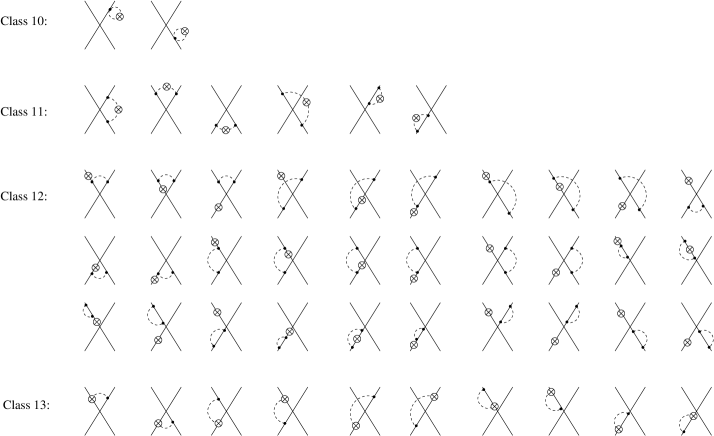
Figure 5: Contributions of the short-range currents. Solid dots are the lowest-order vertices from the effective Lagrangian while the circle-crosses represent insertions of the electromagnetic vertices as explained in the text. For remaining notation see Fig. 1.

We now consider the short-range contributions. The formal structure of the currents involving the leading-order four-nucleon contact interactions $H_{40}^{(2)}$ can be decomposed into four classes $10\ldots 13$ as visualized in Fig. 5. Including the contributions induced by the UTs in Eq. (4.2), we obtain the following algebraic structure:

$$J_{\rm c10} = \eta\biggr{[}H_{22}^{(2)}\frac{\lambda^{2}}{E_{\pi}}H_{40}^{(2)}\frac{\lambda^{2}}{E_{\pi}}J_{02}^{(-1)}-H_{40}^{(2)}\eta H_{22}^{(2)}\frac{\lambda^{2}}{E_{\pi}^{2}}J_{02}^{(-1)}-\bar{\beta}_{1}\biggr{(}H_{22}^{(2)}\frac{\lambda^{2}}{E_{\pi}}H_{40}^{(2)}\frac{\lambda^{2}}{E_{\pi}}J_{02}^{(-1)}-H_{40}^{(2)}\eta H_{22}^{(2)}\frac{\lambda^{2}}{E_{\pi}^{2}}J_{02}^{(-1)}\biggl{)}\biggl{]}\eta+\textrm{h.c.}\,,$$

$$J_{\rm c11} = \eta\biggr{[}H_{40}^{(2)}\eta H_{21}^{(1)}\frac{\lambda^{1}}{E_{\pi}^{2}}J_{02}^{(-1)}\frac{\lambda^{1}}{E_{\pi}}H_{21}^{(1)}-H_{21}^{(1)}\frac{\lambda^{1}}{E_{\pi}}J_{02}^{(-1)}\frac{\lambda^{1}}{E_{\pi}}H_{40}^{(2)}\frac{\lambda^{1}}{E_{\pi}}H_{21}^{(1)}+J_{02}^{(-1)}\frac{\lambda^{2}}{E_{\pi}^{2}}H_{21}^{(1)}\frac{\lambda^{1}}{E_{\pi}}H_{21}^{(1)}\eta H_{40}^{(2)}$$

$$+ J_{02}^{(-1)}\frac{\lambda^{2}}{E_{\pi}}H_{21}^{(1)}\frac{\lambda^{1}}{E_{\pi}^{2}}H_{21}^{(1)}\eta H_{40}^{(2)}-J_{02}^{(-1)}\frac{\lambda^{2}}{E_{\pi}}H_{21}^{(1)}\frac{\lambda^{1}}{E_{\pi}}H_{40}^{(2)}\frac{\lambda^{1}}{E_{\pi}}H_{21}^{(1)}-J_{02}^{(-1)}\frac{\lambda^{2}}{E_{\pi}}H_{40}^{(2)}\frac{\lambda^{2}}{E_{\pi}}H_{21}^{(1)}\frac{\lambda^{1}}{E_{\pi}}H_{21}^{(1)}$$

$$+ \bar{\beta}_{4}\biggr{(}H_{40}^{(2)}\eta H_{21}^{(1)}\frac{\lambda^{1}}{E_{\pi}}H_{21}^{(1)}\frac{\lambda^{2}}{E_{\pi}^{2}}J_{02}^{(-1)}-H_{40}^{(2)}\eta J_{02}^{(-1)}\frac{\lambda^{2}}{E_{\pi}^{2}}H_{21}^{(1)}\frac{\lambda^{1}}{E_{\pi}}H_{21}^{(1)}\biggl{)}+\bar{\beta}_{5}\biggr{(}H_{40}^{(2)}\eta H_{21}^{(1)}\frac{\lambda^{1}}{E_{\pi}^{2}}H_{21}^{(1)}\frac{\lambda^{2}}{E_{\pi}}J_{02}^{(-1)}$$

$$- H_{40}^{(2)}\eta J_{02}^{(-1)}\frac{\lambda^{2}}{E_{\pi}}H_{21}^{(1)}\frac{\lambda^{1}}{E_{\pi}^{2}}H_{21}^{(1)}\biggl{)}+\bar{\beta}_{6}\biggr{(}H_{40}^{(2)}\eta H_{21}^{(1)}\frac{\lambda^{1}}{E_{\pi}^{2}}J_{02}^{(-1)}\frac{\lambda^{1}}{E_{\pi}}H_{21}^{(1)}-H_{40}^{(2)}\eta H_{21}^{(1)}\frac{\lambda^{1}}{E_{\pi}}J_{02}^{(-1)}\frac{\lambda^{1}}{E_{\pi}^{2}}H_{21}^{(1)}\biggl{)}\biggl{]}\eta+\textrm{h.c.}\,,$$

$$J_{\rm c12} = \eta\biggr{[}H_{21}^{(1)}\frac{\lambda^{1}}{E_{\pi}}J_{20}^{(-1)}\frac{\lambda^{1}}{E_{\pi}^{2}}H_{21}^{(1)}\eta H_{40}^{(2)}-H_{21}^{(1)}\frac{\lambda^{1}}{E_{\pi}}H_{40}^{(2)}\frac{\lambda^{1}}{E_{\pi}}J_{20}^{(-1)}\frac{\lambda^{1}}{E_{\pi}}H_{21}^{(1)}-\frac{1}{2}J_{20}^{(-1)}\eta H_{21}^{(1)}\frac{\lambda^{1}}{E_{\pi}^{3}}H_{21}^{(1)}\eta H_{40}^{(2)}$$

$$+ \frac{1}{2}J_{20}^{(-1)}\eta H_{21}^{(1)}\frac{\lambda^{1}}{E_{\pi}^{2}}H_{40}^{(2)}\frac{\lambda^{1}}{E_{\pi}}H_{21}^{(1)}+\frac{1}{2}J_{20}^{(-1)}\eta H_{21}^{(1)}\frac{\lambda^{1}}{E_{\pi}}H_{40}^{(2)}\frac{\lambda^{1}}{E_{\pi}^{2}}H_{21}^{(1)}-\frac{1}{2}J_{20}^{(-1)}\eta H_{40}^{(2)}\eta H_{21}^{(1)}\frac{\lambda^{1}}{E_{\pi}^{3}}H_{21}^{(1)}$$

$$+ \bar{\beta}_{2}\biggr{(}H_{40}^{(2)}\eta H_{21}^{(1)}\frac{\lambda^{1}}{E_{\pi}}J_{20}^{(-1)}\frac{\lambda^{1}}{E_{\pi}^{2}}H_{21}^{(1)}-H_{40}^{(2)}\eta H_{21}^{(1)}\frac{\lambda^{1}}{E_{\pi}^{2}}J_{20}^{(-1)}\frac{\lambda^{1}}{E_{\pi}}H_{21}^{(1)}\biggl{)}+\bar{\beta}_{3}\eta\biggr{(}H_{40}^{(2)}\eta H_{21}^{(1)}\frac{\lambda^{1}}{E_{\pi}^{3}}H_{21}^{(1)}\eta J_{20}^{(-1)}$$

$$- H_{21}^{(1)}\frac{\lambda^{1}}{E_{\pi}^{3}}H_{21}^{(1)}\eta J_{20}^{(-1)}\eta H_{40}^{(2)}\biggl{)}\biggl{]}\eta+\textrm{h.c.}\,,$$

$$J_{\rm c13} = \eta\biggr{[}J_{21}^{(0)}\frac{\lambda^{1}}{E_{\pi}}H_{40}^{(2)}\frac{\lambda^{1}}{E_{\pi}}H_{21}^{(1)}-J_{21}^{(0)}\frac{\lambda^{1}}{E_{\pi}^{2}}H_{21}^{(1)}\eta H_{40}^{(2)}+\bar{\beta}_{7}\,\eta\left(H_{21}^{(1)}\frac{\lambda^{1}}{E_{\pi}^{3}}J_{21}^{(0)}\eta H_{40}^{(2)}-H_{40}^{(2)}\eta H_{21}^{(1)}\frac{\lambda^{1}}{E_{\pi}^{3}}J_{21}^{(0)}\right)\biggl{]}\eta+\textrm{h.c.}\,.$$ (5.1)

We found that only the class-11 matrix elements yield non-vanishing contributions to the current density:

$$\vec{J}_{\rm c11}=-e\frac{g_{A}^{2}\,i}{4F_{\pi}^{2}}\,C_{T}\int\frac{d^{3}l}{(2\pi)^{3}}\,\vec{l}\biggl{[}2\,\vec{l}\cdot\left[\vec{k}\times\vec{\sigma}_{1}\right]\tau_{2}^{3}+\vec{\sigma}_{1}\cdot\vec{l}\,\vec{\sigma}_{2}\cdot\vec{k}\left[\vec{\tau}_{1}\times\vec{\tau}_{2}\right]^{3}\biggr{]}\frac{\omega_{+}^{2}+\omega_{+}\omega_{-}+\omega_{-}^{2}}{\omega_{+}^{3}\omega_{-}^{3}(\omega_{+}+\omega_{-})}\,.$$ (5.2)

We find, however, that the resulting contribution to the current vanishes after performing antisymmetrization of the two-nucleon states.

The tree contributions emerge from gauging the subleading contact interactions in the Lagrangian $\mathcal{L}_{NN}^{(2)}$ and the two new gauge-invariant terms proportional to the LECs $L_{1,2}$:

$$\vec{J}_{\rm contact} = e\,\frac{i}{16}\left[\vec{\tau}_{1}\times\vec{\tau}_{2}\right]^{3}\,\biggl{[}\left(C_{2}+3C_{4}+C_{7}\right)\,\vec{q}_{1}-\left(-C_{2}+C_{4}+C_{7}\right)\,\,\left(\vec{\sigma}_{1}\cdot\vec{\sigma}_{2}\right)\,\,\vec{q}_{1}+C_{7}\,\left(\vec{\sigma}_{2}\cdot\vec{q}_{1}\,\vec{\sigma}_{1}+\,\vec{\sigma}_{1}\cdot\vec{q}_{1}\,\vec{\sigma}_{2}\right)\biggr{]}$$ (5.3)

$$- e\,\frac{C_{5}\,i}{16}\,\tau_{1}^{3}\,\left[\left(\vec{\sigma}_{1}+\vec{\sigma}_{2}\right)\times\vec{q}_{1}\right]+ieL_{1}\,\tau_{1}^{3}\,\left[\left(\vec{\sigma}_{1}-\vec{\sigma}_{2}\right)\times\vec{k}\right]+ieL_{2}\,\left[\left(\vec{\sigma}_{1}+\vec{\sigma}_{2}\right)\times\vec{q}_{1}\right]\,.$$

It is reassuring to note that all the divergences of the two-pion exchange loop integrals are cancelled by the same redefinition of $C_{i}$ that is needed to renormalize the potential Epelbaum:2003gr . From the two LECs that are genuine to the current operator, only $L_{1}$ gets renormalized. Employing DR and the $\overline{\textrm{MS}}$-scheme, the relation between the bare and renormalized LEC $L_{1}$ has the form

$$L_{1} = \bar{L}_{1}+\frac{g_{A}^{2}-3g_{A}^{4}}{8F_{\pi}^{4}}\Delta_{\pi}\,.$$ (5.4)

The charge density is completely given by the class-11,12 loop diagrams:

$$\rho_{\rm c11} = -e\frac{g_{A}^{2}}{4F_{\pi}^{2}}\,C_{T}\,\tau_{1}^{3}\int\frac{d^{3}l}{(2\pi)^{3}}\left(\vec{\sigma}_{1}\cdot\vec{\sigma}_{2}\,(k^{2}-l^{2})-\vec{\sigma}_{1}\cdot\vec{k}\,\vec{\sigma}_{2}\cdot\vec{k}+\vec{\sigma}_{1}\cdot\vec{l}\,\vec{\sigma}_{2}\cdot\vec{l}\,\right)\frac{1}{\omega_{+}^{2}\omega_{-}^{2}}\,,$$

$$\rho_{\rm c12} = -e\frac{g_{A}^{2}}{3F_{\pi}^{2}}\,C_{T}\,\,\tau_{1}^{3}\vec{\sigma}_{1}\cdot\vec{\sigma}_{2}\int\frac{d^{3}l}{(2\pi)^{3}}\frac{l^{2}}{\omega_{l}^{4}}\,.$$ (5.5)

In DR, the integrals entering these expressions are finite, and the result for the short-range charge density reads

$$\rho_{\rm contact}=C_{T}\,\tau_{1}^{3}\,\left[\vec{\sigma}_{1}\cdot\vec{k}\,\vec{\sigma}_{2}\cdot\vec{k}\,f_{9}(k)+\vec{\sigma}_{1}\cdot\vec{\sigma}_{2}\,f_{10}(k)\right]\,,$$ (5.6)

where

$$f_{9}(k) = e\frac{g_{A}^{2}}{32F_{\pi}^{2}\pi}\left(A(k)+\frac{M_{\pi}-4M_{\pi}^{2}\,A(k)}{k^{2}}\right)\,,$$

$$f_{10}(k) = e\frac{g_{A}^{2}}{32F_{\pi}^{2}\pi}\,\left(M_{\pi}-(4M_{\pi}^{2}+3k^{2})\,A(k)\right)\,.$$ (5.7)

Notice that for antisymmetric nuclear states, the two structures in Eq. (5.6) can be combined into a single one. Equations (5.3) and (5.6) represent our final results for the short-range contributions.

VI Comparison with the work by Pastore et al.

We now compare our results given in the previous sections with the ones obtained by Pastore et al. Pastore:2008ui ; Pastore:2009is ; Pastore:2011ip . Below, we list the (numerous) differences and, in some cases, comment on their possible origin.

• We begin with the exchange current density given in Eq. (4.28). Our result for the pion loop contributions (i.e. terms proportional to the loop function $L(k)$) agrees with the one of Pastore:2009is for the class-9 operator, see the contribution $\propto L(k)$ in $f_{5}$. As Pastore et al., we also find, that the class-8 operator is cancelled by a part of the class-5 operator. The rest of the class-5 operator is not mentioned in Pastore:2009is . As shown in section IV.3, this part vanishes in our treatment due to the renormalizability constraint. For the seagull current, see the contribution $\propto L(k)$ in $f_{3}$, we obtain a completely different result with even a different isospin dependence: $[\vec{\tau}_{1}\times\vec{\tau}_{2}]^{3}$ as compared to $\tau_{1,2}^{3}$ in Pastore:2009is , see Eq. (3.36) in their work. This should not come as a surprise given the fact that Pastore et al. did not succeed to extract the (truly) irreducible part of the amplitude for this particular topology, see the discussion in appendix E of Pastore:2009is . In particular, they even encountered some non-Hermitian contributions which then were ignored.

• We also disagree on the tree contributions to the current density except the one $\propto d_{21}$. In particular, our terms $\propto d_{8,9}$ have a different sign. Further, we find independent contributions from both LECs $d_{21}$ and $d_{22}$, while in Pastore:2009is they only appear in a linear combination $2d_{21}+d_{22}$. Finally, Pastore et al. miss the contributions from the LEC $d_{18}$ (which accounts for the Goldberger-Treiman discrepancy) and $l_{6}$. Last but not least, we emphasize that our result for the current operator in Eq. (4.28) depends on renormalized LECs $\bar{d}_{8,9,18,21,22}$ and $\bar{l}_{6}$ which, of course, can be taken from other reactions such as e.g. pion-nucleon scattering Fettes:2001cr .

• We now turn to the one-pion exchange charge density operator given in Eq. (4.30). The expressions for the leading relativistic corrections $\propto 1/m_{N}$ are, of course, not new and agree with the ones given in Pastore:2011ip . We, however, also obtain nonvanishing pion loop contributions to the exchange charge density, see the $f_{7,8}$ terms in Eq. (4.30), which are not considered in Ref. Pastore:2011ip .

• Finally, our expressions for the pion loop contribution to the short-range current and charge operators also strongly disagree with the ones given in Refs. Pastore:2009is and Pastore:2011ip , respectively. In particular, the results obtained by Pastore et al. depend on both leading-order LECs $C_{S}$ and $C_{T}$, while there is no dependence on $C_{S}$ in our case. Morover, we find that the short-range pion loop contribution to the current density vanishes completely upon performing antisymmetrization. The origin of these discrepancies might be related to the unitary ambiguity of the nuclear potential and current operators. As discussed in the previous sections, we include in our derivation a large number of additional UTs which are possible at the given order in the chiral expansion. In particular, pion loop contributions to short-range current/charge operators are affected by the strong UT defined in Eq. (3.48) of Ref. Epelbaum:2007us and $\mathcal{A_{\mu}}$-dependent UTs which induce additional operators listed in Eq. (V). As a consequence, the resulting short-range currents might be expected to be strongly scheme dependent (i.e. dependent on the a priori unknown angles of these additional UTs). It is the renormalizability requirement of the nuclear potentials and currents that provides strong constraints on the choice of the additional UTs, see the detailed discussion in Refs. Kolling:2009iq ; Epelbaum:2007us and in section II, and leads finally to unambiguous expressions for the (static) nuclear potentials and current/charge operators at the considered order. The observed differences for the short-range operators suggest that the results of Ref. Pastore:2011ip might correspond to a different choice of the additional UTs as compared to the one adopted in our work. Our findings, however, imply that such a different choice would result in impossibility to obtain renormalized expressions for the nuclear forces and/or the current operator.

VII Summary

The results of our work can be summarized as follows:

• We applied the method of unitary transformation to work out the leading loop contributions to the one-pion exchange and short-range two-nucleon electromagnetic current and charge densities. The renormalized expressions for the one-pion exchange charge and current operators are given for the first time.

• We discuss in detail renormalization of the one-pion exchange contributions which provides a stringent test of our theoretical approach. More precisely, all emerging ultraviolet divergences have to be absorbed into redefinition of the low-energy constants $l_{i}$ and $d_{i}$ entering the Lagrangians $\mathcal{L}_{\pi\pi}^{(4)}$ and $\mathcal{L}_{\pi N}^{(3)}$, respectively. There is no freedom in this procedure as the corresponding $\beta$-functions of all these LECs in DR are fixed and well known. We demonstrate, that it is indeed possible to renormalize the one-loop contributions provided one makes use of the freedom to employ additional unitary transformations.

• We succeeded to obtain compact, analytical expressions for the current and charge densities both in momentum and coordinate spaces which can be used in future numerical calculations.

• Finally, we provide a detailed comparison between our results and the ones obtained by Pastore et al. within a different framework.

The final results of our work are summarized in Eqs. (4.28), (4.30), (5.3) and (5.6) which contain the expressions for the one-pion exchange and short-range contributions to the two-nucleon current and charge densities at order $eQ$ (leading loop order). It would be interesting to explore effects of these novel contributions to the exchange current and charge densities in e.g. electron scattering off light nuclei. This work is in progress, see also Rozpedzik:2011cx for a pioneering calculation along this line concentrating on the two-pion exchange contributions.

Appendix A Hamilton density

In this appendix we define the expressions for the Hamilton density and currents. First let us recapitulate the expressions we already defined in Kolling:2009iq

$$\mathcal{H}_{21}^{(1)} = \frac{\mathring{g}_{A}}{2F}N^{\dagger}\left(\vec{\sigma}\vec{\tau}\cdot\cdot\vec{\nabla}\vec{\pi}\right)N\,,$$

$$\mathcal{H}_{22}^{(2)} = \frac{1}{4F^{2}}N^{\dagger}\big{[}\vec{\pi}\times\dot{\vec{\pi}}\big{]}\cdot\vec{\tau}N\,,$$

$$\mathcal{H}_{42}^{(4)} = \frac{1}{32F^{4}}\left(N^{\dagger}\left[\vec{\tau}\times\vec{\pi}\right]N\right)\cdot\left(N^{\dagger}\left[\vec{\tau}\times\vec{\pi}\right]N\right)\,,$$

$${J^{0}_{20}}^{(-1)} = \frac{e}{2}N^{\dagger}\left(\mathbbm{1}+\tau_{3}\right)N=eN^{\dagger}\,\hat{e}\,N\,,$$

$${J_{02}^{0}}^{(-1)} = e\big{[}\vec{\pi}\times\dot{\vec{\pi}}\big{]}_{3}\,,$$

$${\vec{J}_{02}\,}^{(-1)} = -e\big{[}\vec{\pi}\times\vec{\nabla}\vec{\pi}\big{]}_{3}\,,$$

$${\vec{J}_{21}\,}^{(0)} = e\,\frac{\mathring{g}_{A}}{2F}N^{\dagger}\vec{\sigma}\left[\vec{\tau}\times\vec{\pi}\right]_{3}N\,.$$ (A.1)

The definitions of the other parts of the Hamiltonian density and currents is given below.

$$\mathcal{H}_{23}^{(3)} = \frac{\mathring{g}_{A}}{4F^{3}}N^{\dagger}\left[2\,\vec{\sigma}\vec{\tau}\cdot\cdot\vec{\nabla}\vec{\pi}\,\vec{\pi}^{\,2}\,\xi+(1-4\xi)\vec{\tau}\cdot\vec{\pi}\,\vec{\sigma}\cdot\vec{\nabla}\vec{\pi}^{\,2}\right]N\,,$$

$$\mathcal{H}_{04}^{(2)} = \frac{1}{8F^{2}}N^{\dagger}\left[8\xi\,\partial_{\mu}\vec{\pi}\cdot\partial^{\mu}\vec{\pi}\,\vec{\pi}^{\,2}-(1-4\xi)\left(\vec{\pi}\cdot\partial_{\mu}\vec{\pi}\right)^{2}-(8\xi-1)M_{\pi}^{2}\,\vec{\pi}^{\,4}\right]\,,$$

$$\mathcal{H}_{04}^{(2)} = \frac{C_{S}}{2}N^{\dagger}N\,N^{\dagger}N+\frac{C_{T}}{2}N^{\dagger}\,\vec{\sigma}N\cdot N^{\dagger}\,\vec{\sigma}N\,,$$

$$\mathcal{H}_{21}^{(3)} = \frac{2d_{16}-d_{18}}{F}M_{\pi}^{2}\,N^{\dagger}\vec{\sigma}\vec{\tau}\cdot\cdot\vec{\nabla}\vec{\pi}N\,,$$

$$\tilde{\mathcal{H}}_{21}^{(3)} = -\frac{\mathring{g}_{A}i}{4m_{N}F}N^{\dagger}\vec{\sigma}\cdot\overleftrightarrow{\nabla}\,\vec{\tau}\cdot\dot{\vec{\pi}}N\,,$$

$$\tilde{\mathcal{H}}_{20}^{(2)} = -\frac{1}{2m_{N}}N^{\dagger}\vec{\nabla}^{\,2}N\,,$$

$${J^{0}_{02}}^{(1)} = -2ie\frac{l_{6}}{F^{2}}\epsilon_{3ab}\,\vec{k}\cdot\vec{\nabla}\pi_{a}\,\dot{\pi}_{b}\,,$$

$${\vec{J}_{02}\,}^{(1)} = 2ie\epsilon_{3ab}\,\left(\frac{l_{6}}{F^{2}}\,\vec{\nabla}\pi_{a}\,\vec{k}\cdot\vec{\nabla}\pi_{b}+il_{4}\frac{M_{\pi}^{2}}{F^{2}}\pi_{a}\vec{\nabla}\pi_{b}\right)\,,$$

$${J^{0}_{20}\,}^{(1)} = e\vec{k}^{\,2}N^{\dagger}(d_{6}\tau_{3}+2d_{7})N\,,$$

$${\tilde{\vec{J}}_{20}}^{(1)} = -\frac{ie}{4m_{N}}N^{\dagger}\left[(\mathbbm{1}+\tau^{3})\overleftrightarrow{\nabla}+(1+c_{6})\,(\mathbbm{1}+\tau^{3})\vec{\sigma}\times\vec{k}+2c_{7}\,\vec{\sigma}\times\vec{k}\right]N\,,$$

$${\tilde{\vec{J}}_{20}}^{(1)} = -\frac{ie}{4m_{N}}N^{\dagger}(\mathbbm{1}+\tau^{3})\overleftrightarrow{\nabla}N\,,$$

$${J^{0}_{21}}^{(2)} = -e\frac{i}{F}N^{\dagger}\epsilon_{3ab}\tau_{b}(d_{20}+d_{21}-\frac{d_{22}}{2})\vec{\sigma}\cdot\vec{k}\,\dot{\pi}_{a}N\,,$$

$${\vec{J}_{21}\,}^{(2)} = \frac{e}{F}N^{\dagger}\biggl{[}-4id_{8}\vec{k}\times\vec{\nabla}\pi_{3}-4id_{9}\vec{k}\times\vec{\nabla}\pi_{a}\,\tau_{a}+\epsilon_{3ab}\tau_{b}\biggl{(}-\vec{\sigma}\pi_{a}(2d_{16}-d_{18})\,M_{\pi}^{2}$$

$${}+i\left(d_{21}-\frac{d_{22}}{2}\right)\,\vec{k}\times\left[\vec{\sigma}\times\vec{\nabla}\right]\pi_{a}-\frac{d_{22}}{2}\pi_{a}\vec{k}\times\left[\vec{k}\times\vec{\sigma}\right]\biggr{)}\biggr{]}N\,,$$

$${\tilde{\vec{J}}_{21}}^{(2)} = -\frac{e\mathring{g}_{A}}{4m_{N}F}N^{\dagger}\vec{\sigma}(\tau_{a}+\delta_{a3})\dot{\pi}_{a}N\,.$$ (A.2)

Appendix B Loop integrals

The following integrals contribute to the one-pion exchange current operator at the leading one-loop order:

$$\int\frac{d^{3}l}{(2\pi)^{3}}\frac{1}{\omega_{l}} = 2\Delta_{\pi}\,,$$

$$\int\frac{d^{3}l}{(2\pi)^{3}}\frac{l^{2}}{\omega_{l}^{3}} = 6\Delta_{\pi}\,,$$

$$\int\frac{d^{3}l}{(2\pi)^{3}}\frac{l^{2}}{\omega_{l}^{4}} = -\frac{3M_{\pi}}{8\pi}\,,$$

$$\int\frac{d^{3}l}{(2\pi)^{3}}\frac{l^{a}\,l^{b}}{\omega_{+}\omega_{-}(\omega_{+}+\omega_{-})} \equiv \mathcal{I}_{2}\,\delta^{ab}+k^{a}k^{b}\,\mathcal{I}_{3}\,,$$

$$\int\frac{d^{3}l}{(2\pi)^{3}}\frac{\omega_{-}-\omega_{+}}{\omega_{+}\omega_{-}(\omega_{+}+\omega_{-})^{2}}l^{a} \equiv k^{a}\,\mathcal{K}_{1}\,,$$

$$\int\frac{d^{3}l}{(2\pi)^{3}}\frac{2\omega_{+}+\omega_{-}}{\omega_{-}\omega_{+}^{3}(\omega_{+}+\omega_{-})^{2}}l^{a} \equiv k^{a}\mathcal{B}_{1}\,,$$

$$\int\frac{d^{3}l}{(2\pi)^{3}}\frac{2\omega_{+}+\omega_{-}}{\omega_{-}\omega_{+}^{3}(\omega_{+}+\omega_{-})^{2}}l^{a}l^{b} \equiv \delta^{ab}\mathcal{B}_{2}+k^{a}k^{b}\mathcal{B}_{3}\,,$$

$$\int\frac{d^{3}l}{(2\pi)^{3}}\frac{2\omega_{+}+\omega_{-}}{\omega_{-}\omega_{+}^{3}(\omega_{+}+\omega_{-})^{2}}l^{a}l^{b}l^{c} \equiv (\delta^{ab}k^{c}+\delta^{ac}k^{b}+\delta^{bc}k^{a})\mathcal{B}_{4}+k^{a}k^{b}k^{c}\mathcal{B}_{5}\,,$$

$$\int\frac{d^{3}l}{(2\pi)^{3}}\frac{1}{\omega_{+}^{2}\omega_{-}^{2}} \equiv \mathcal{A}_{0}\,,$$

$$\int\frac{d^{3}l}{(2\pi)^{3}}\frac{l^{a}\,l^{b}}{\omega_{+}^{2}\omega_{-}^{2}} \equiv \mathcal{A}_{2}\delta^{ab}+\mathcal{A}_{3}k^{a}\,k^{b}\,,$$ (B.1)

where the pion energies $\omega_{l}$ and $\omega_{\pm}$ are defined as

$$\omega_{l}=\sqrt{l^{2}+M_{\pi}^{2}}\,,\qquad\omega_{\pm}=\sqrt{\left(\vec{l}\pm\vec{k}\right)^{2}+4M_{\pi}^{2}}\,.$$ (B.2)

The integrals can be computed explicitly in dimensional regularization. We only give here the results for the integrals that are actually needed. These are:

$$\mathcal{I}_{2} = \left(4+\frac{2k^{2}}{3M_{\pi}^{2}}\right)\Delta_{\pi}+\frac{s^{2}L(k)}{12\pi^{2}}-\frac{5k^{2}+24M_{\pi}^{2}}{72\pi^{2}}\,,$$

$$\mathcal{I}_{3} = -\mathcal{K}_{1}=-2\mathcal{B}_{4}=-\frac{2\Delta_{\pi}}{3M_{\pi}^{2}}-\frac{s^{2}L(k)}{12\pi^{2}k^{2}}+\frac{5k^{2}+24M_{\pi}^{2}}{72\pi^{2}k^{2}}\,,$$

$$\mathcal{B}_{1} = -\mathcal{B}_{3}=-\frac{L(k)-1}{8\pi^{2}k^{2}}\,,$$

$$\mathcal{B}_{2} = -\frac{\Delta_{\pi}}{M_{\pi}^{2}}-\frac{2L(k)-1}{16\pi^{2}}\,,$$

$$\mathcal{B}_{5} = -\frac{(4M_{\pi}^{2}+k^{2})L(k)}{8\pi^{2}k^{4}}+\frac{3M_{\pi}^{2}+k^{2}}{6\pi^{2}k^{4}}\,,$$

$$\mathcal{A}_{0} = \frac{A(k)}{4\pi}\,,$$

$$\mathcal{A}_{2} = -\frac{M_{\pi}+s^{2}A(k)}{8\pi}\,,$$

$$\mathcal{A}_{3} = -\frac{M_{\pi}-s^{2}A(k)}{8\pi k^{2}}\,.$$ (B.3)

where we have introduced

$$L(k)=\frac{1}{2}\frac{s}{k}\log\left(\frac{s+k}{s-k}\right),\qquad A(k)=\frac{1}{2k}\arctan\left(\frac{k}{2M_{\pi}}\right),\qquad s=\sqrt{k^{2}+4M_{\pi}^{2}},$$ (B.4)

with $k=|\vec{k}\,|$. Further, the integral $\Delta_{\pi}$ is defined in Ref. Bernard:1995dp according to

$$\Delta_{\pi}=\lim_{d\to 4}\frac{1}{i}\int\frac{d^{d}l}{\left(2\pi\right)^{d}}\frac{1}{M_{\pi}^{2}-l^{2}-i\epsilon}=2M_{\pi}^{2}\left(\lim_{d\to 4}L+\frac{1}{16\pi^{2}}\log\left(\frac{M_{\pi}}{\mu}\right)\right),$$ (B.5)

where the quantity $L$ has a pole in $d=4$ dimensions and is given by

$$L=\frac{\mu^{d-4}}{16\pi^{2}}\left[\frac{1}{d-4}-\frac{1}{2}\left(\Gamma^{\prime}(1)+1+\log\left(4\pi\right)\right)\right].$$ (B.6)

Appendix C Configuration-Space Expressions

For the sake of completeness, we also give the expressions in configuration space obtained by carrying out the Fourier-transformation of the momentum space results

$$\mathcal{F}\left(f(\vec{q}_{1}\,,\,\vec{q}_{2}\,)\right)\equiv\int\frac{d^{3}q_{1}}{(2\pi)^{3}}\frac{d^{3}q_{2}}{(2\pi)^{3}}e^{i\vec{q}_{1}\cdot\vec{r}_{1}}e^{i\vec{q}_{2}\cdot\vec{r}_{2}}\,f(\vec{q}_{1}\,,\,\vec{q}_{2}\,)\,(2\pi)^{3}\,\delta^{3}\left(\vec{q}_{1}+\vec{q}_{2}-\vec{k}\right)\,.$$ (C.1)

We find the following expressions:

$$\vec{J}_{1\pi} = \biggl{(}-\left[\tau_{2}^{3}\,f_{1}(k)+\vec{\tau}_{1}\cdot\vec{\tau}_{2}\,f_{2}(k)\right]\,\vec{\sigma}_{2}\cdot\vec{\nabla}_{12}\,\left[\vec{k}\times\vec{\nabla}_{12}\right]+\left[\vec{\tau}_{1}\times\vec{\tau}_{2}\right]^{3}\vec{\sigma}_{2}\cdot\vec{\nabla}_{12}\biggl{[}-\vec{k}\times\left[\vec{\nabla}_{12}\times\vec{\sigma}_{1}\right]f_{3}(k)\,$$ (C.2)

$$+ \vec{k}\times\left[\left(\vec{\nabla}_{12}\,+i\vec{k}\right)\times\vec{\sigma}_{1}\right]\,f_{4}(k)+\vec{\sigma}_{1}\cdot\left(\vec{\nabla}_{12}+i\vec{k}\right)\,\frac{\vec{k}}{k^{2}}\,f_{5}(k)-i\vec{\sigma}_{1}\,f_{6}(k)\biggl{]}\biggl{)}\,\frac{M_{\pi}e^{-M_{\pi}\,r_{12}}}{4\pi\,r_{12}}e^{i\vec{k}\cdot\vec{r}_{1}}$$

$$+ \frac{i}{2}\,\left[\vec{\tau}_{1}\times\vec{\tau}_{2}\right]^{3}\vec{\sigma}_{2}\cdot\left(\vec{\nabla}_{12}-\frac{i\vec{k}}{2}\right)\,\vec{\sigma}_{1}\cdot\left(\vec{\nabla}_{12}+\frac{i\vec{k}}{2}\right)\,\biggl{[}f_{5}(k)-f_{6}(k)\biggl{]}\,\vec{\nabla}_{12}\,f\left(\vec{k},\vec{r}_{12}\right)e^{i\vec{k}\cdot\vec{R}}\,,$$

where we have introduced

$$\vec{r}_{12} = \vec{r}_{1}-\vec{r}_{2}\,,\qquad\vec{R}=\frac{\vec{r}_{1}+\vec{r}_{2}}{2}\,,\qquad\vec{\nabla}_{12}=\vec{\nabla}_{r_{12}}\,,$$

$$f\left(\vec{k},\vec{r}_{12}\right) = \int\frac{d^{3}p}{(2\pi)^{3}}\int_{-1}^{1}dx\,\frac{e^{i\vec{r}_{12}\cdot\left(\vec{p}+\vec{k}\,x/2\right)}}{(p^{2}+M_{\pi}^{2}+(1-x^{2})k^{2}/4)^{2}}\,.$$ (C.3)

The one-pion exchange charge density has the following form:

$$\rho_{1\pi} = \biggl{(}-2M_{\pi}^{2}\,\vec{\sigma}_{2}\cdot\vec{\nabla}_{12}\tau_{2}^{3}\biggr{[}\vec{\sigma}_{1}\cdot\vec{k}\,\vec{\nabla}_{12}\cdot\vec{k}\,f_{7}(k)+\vec{\nabla}_{12}\cdot\vec{\sigma}_{1}\,f_{8}(k)\biggl{]}\,+\,\frac{ieg_{A}^{2}\,M_{\pi}^{2}}{8F_{\pi}^{2}m_{N}}\biggl{[}(1-2\bar{\beta}_{9})\left(\tau_{2}^{3}+\vec{\tau}_{1}\cdot\vec{\tau}_{2}\right)\vec{\sigma}_{1}\cdot\vec{k}\vec{\sigma}_{2}\cdot\vec{\nabla}_{12}$$ (C.4)

$$- i(1+2\bar{\beta}_{9})\left[\vec{\tau}_{1}\times\vec{\tau}_{2}\right]^{3}\left(\vec{\sigma}_{1}\cdot\vec{k}_{1}\vec{\sigma}_{2}\cdot\vec{\nabla}_{12}-\vec{\sigma}_{2}\cdot\vec{k}_{2}\vec{\sigma}_{1}\cdot\vec{\nabla}_{12}\right)\biggr{]}-\frac{ieg_{A}^{2}}{16m_{N}F_{\pi}^{2}}\vec{\sigma}_{1}\cdot\vec{\nabla}_{12}\,\vec{\sigma}_{2}\cdot\vec{\nabla}_{12}\,\biggl{[}(2\bar{\beta}_{8}-1)(\tau_{2}^{3}+\left(\vec{\tau_{1}}\cdot\vec{\tau}_{2}\right))\,$$

$$\times \vec{\nabla}_{12}\cdot\vec{k}+i\left[\vec{\tau}_{1}\times\vec{\tau}_{2}\right]^{3}\biggl{(}-\left(2\bar{\beta}_{8}+1\right)\vec{\nabla}_{12}\cdot\vec{k}_{2}+\left(2\bar{\beta}_{8}-1\,\right)\,\vec{\nabla}_{12}\cdot\vec{k}_{1}\,\biggr{)}\biggr{]}\biggr{)}\,\frac{e^{-M_{\pi}r_{12}}}{8\pi\,M_{\pi}\,r_{12}}e^{i\vec{k}\cdot\vec{r}_{1}}$$

$$+ e\frac{g_{A}^{2}}{16F_{\pi}^{2}m_{N}}\,\left[\vec{\tau}_{1}\times\vec{\tau}_{2}\right]^{3}\,\vec{\sigma}_{1}\cdot\left(\vec{\nabla}_{12}+\frac{i\vec{k}}{2}\right)\,\vec{\sigma}_{2}\cdot\left(\vec{\nabla}_{12}-\frac{i\vec{k}}{2}\right)\,\left(\vec{\nabla}_{12}+\frac{i\vec{k}}{2}\right)\cdot\vec{k}_{1}\,f\left(\vec{k},\vec{r}_{12}\right)\,e^{i\vec{k}\cdot\vec{R}}\,.$$

Finally, we also give the coordinate-space expression for the short-range currents:

$$\rho_{\rm contact} = C_{T}\,\tau_{1}^{3}\,\left[\vec{\sigma}_{1}\cdot\vec{k}\,\vec{\sigma}_{2}\cdot\vec{k}\,\frac{2g_{A}^{2}}{F_{\pi}^{2}}\,f_{9}\left(k\right)+\vec{\sigma}_{1}\cdot\vec{\sigma}_{2}\,f_{10}\left(k\right)\right]e^{i\vec{k}\cdot\vec{R}}\delta^{3}\left(\vec{r}_{12}\right)\,,$$ (C.5)

$$\vec{J}_{\rm contact} = \biggl{\{}e\,\frac{1}{16}\left[\vec{\tau}_{1}\times\vec{\tau}_{2}\right]^{3}\,\biggl{[}\left(C_{2}+3C_{4}+C_{7}\right)\vec{\nabla}_{12}-\left(-C_{2}+C_{4}+C_{7}\right)\,\,\left(\vec{\sigma}_{1}\cdot\vec{\sigma}_{2}\right)\,\vec{\nabla}_{12}$$

$$+ C_{7}\,\left(\vec{\sigma}_{2}\cdot\vec{\nabla}_{12}\,\vec{\sigma}_{1}+\,\vec{\sigma}_{1}\cdot\vec{\nabla}_{12}\,\vec{\sigma}_{2}\right)\biggr{]}-e\,\frac{C_{5}\,}{16}\,\tau_{1}^{3}\,\left[\left(\vec{\sigma}_{1}+\vec{\sigma}_{2}\right)\times\vec{\nabla}_{12}\right]+ieL_{1}\,\tau_{1}^{3}\,\left[\left(\vec{\sigma}_{1}-\vec{\sigma}_{2}\right)\times\vec{k}\right]$$

$$+ ieL_{2}\,\left[\vec{\sigma}_{1}\times\vec{k}\right]\biggr{\}}e^{i\vec{k}\cdot\vec{R}}\delta^{3}\left(\vec{r}_{12}\right)\,.$$

References

• (1) S. Pastore, R. Schiavilla, J. L. Goity, Phys. Rev.  C78, 064002 (2008). [arXiv:0810.1941 [nucl-th]].
• (2) S. Pastore, L. Girlanda, R. Schiavilla, M. Viviani and R. B. Wiringa, Phys. Rev.  C 80, 034004 (2009) [arXiv:0906.1800 [nucl-th]].
• (3) S. Kölling, E. Epelbaum, H. Krebs and U.-G. Meißner, Phys. Rev.  C 80, 045502 (2009) [arXiv:0907.3437 [nucl-th]].
• (4) S. Pastore, L. Girlanda, R. Schiavilla, M. Viviani, [arXiv:1106.4539 [nucl-th]].
• (5) T.-S. Park, D.-P. Min, M. Rho, Nucl. Phys.  A596, 515 (1996). [nucl-th/9505017].
• (6) S. Weinberg, Nucl. Phys.  B363, 3 (1991).
• (7) E. Epelbaum, H.-W. Hammer, U.-G. Meißner, Rev. Mod. Phys.  81, 1773 (2009). [arXiv:0811.1338 [nucl-th]].
• (8) E. Epelbaum, W. Gloeckle, U.-G. Meißner, Nucl. Phys.  A637, 107 (1998). [nucl-th/9801064].
• (9) E. Epelbaum, W. Gloeckle, U.-G. Meißner, Nucl. Phys.  A671, 295 (2000). [nucl-th/9910064].
• (10) E. Epelbaum, U.-G. Meißner and W. Glöckle, Nucl. Phys.  A 714, 535 (2003) [arXiv:nucl-th/0207089].
• (11) I. S. Gerstein, R. Jackiw, S. Weinberg and B. W. Lee, Phys. Rev.  D 3, 2486 (1971).
• (12) E. Epelbaum, Eur. Phys. J.  A 34, 197 (2007) [arXiv:0710.4250 [nucl-th]].
• (13) E. Epelbaum, Phys. Lett.  B 639, 456 (2006) [arXiv:nucl-th/0511025].
• (14) J. Gasser, H. Leutwyler, Annals Phys.  158, 142 (1984).
• (15) S. Bellucci, J. Gasser and M. E. Sainio, Nucl. Phys.  B 423, 80 (1994) [Erratum-ibid.  B 431, 413 (1994)] [arXiv:hep-ph/9401206].
• (16) G. Ecker and M. Mojžiš, Phys. Lett.  B 365, 312 (1996) [arXiv:hep-ph/9508204].
• (17) N. Fettes, U.-G. Meißner and S. Steininger, Nucl. Phys.  A 640, 199 (1998) [arXiv:hep-ph/9803266].
• (18) N. Fettes, U.-G. Meißner, M. Mojžiš and S. Steininger, Annals Phys.  283, 273 (2000) [Erratum-ibid.  288, 249 (2001)] [arXiv:hep-ph/0001308].
• (19) J. Gasser, M. A. Ivanov, E. Lipartia, M. Mojžiš and A. Rusetsky, Eur. Phys. J.  C 26, 13 (2002) [arXiv:hep-ph/0206068].
• (20) E. Epelbaum, “The nucleon nucleon interaction in a chiral effective field theory,” PhD thesis, University of Bochum, 2000.
• (21) L. Girlanda, S. Pastore, R. Schiavilla and M. Viviani, Phys. Rev.  C 81, 034005 (2010) [arXiv:1001.3676 [nucl-th]].
• (22) C. Ordonez, L. Ray, U. van Kolck, Phys. Rev.  C53, 2086 (1996). [hep-ph/9511380].
• (23) J. L. Friar, Phys. Rev.  C60, 034002 (1999). [nucl-th/9901082].
• (24) J. Adam, H. Goller, H. Arenhövel, Phys. Rev.  C48, 370 (1993).
• (25) E. Epelbaum, W. Glockle and U.-G. Meißner, Nucl. Phys.  A 747, 362 (2005) [arXiv:nucl-th/0405048].
• (26) E. Epelbaum, W. Glöckle, and U.-G. Meißner, Eur. Phys. J. A19, 125 (2004) [arXiv:nucl-th/0304037]
• (27) V. Bernard, N. Kaiser and U.-G. Meißner, Int. J. Mod. Phys.  E 4, 193 (1995) [arXiv:hep-ph/9501384].
• (28) V. Bernard, E. Epelbaum, H. Krebs and U.-G. Meißner, Phys. Rev.  C 77, 064004 (2008) [arXiv:0712.1967 [nucl-th]].
• (29) J. A. Eden and M. F. Gari, Phys. Rev.  C 53, 1102 (1996) [arXiv:nucl-th/9506001].
• (30) N. Fettes, U.-G. Meißner, Nucl. Phys.  A693, 693 (2001). [hep-ph/0101030].
• (31) D. Rozpedzik, J. Golak, S. Kölling, E. Epelbaum, R. Skibinski, H. Witala, H. Krebs, Phys. Rev.  C 83, 064004 (2011) [arXiv:1103.4062 [nucl-th]].