Radius of Close-to-convexity of Harmonic Functions

Abstract.

Let ${\mathcal{H}}$ denote the class of all normalized complex-valued harmonic functions $f=h+\overline{g}$ in the unit disk ${\mathbb{D}}$, and let $K=H+\overline{G}$ denote the harmonic Koebe function. Let $a_{n},b_{n},A_{n},B_{n}$ denote the Maclaurin coefficients of $h,g,H,G$, and

$${\mathcal{F}}=\{f=h+\overline{g}\in{\mathcal{H}}:\,|a_{n}|\leq A_{n}~{}\mbox{ and }~{}|b_{n}|\leq B_{n}~{}\mbox{ for }~{}n\geq 1\}.$$

We show that the radius of univalence of the family ${\mathcal{F}}$ is $0.112903\ldots$. We also show that this number is also the radius of the starlikeness of ${\mathcal{F}}$. Analogous results are proved for a subclass of the class of harmonic convex functions in ${\mathcal{H}}$. These results are obtained as a consequence of a new coefficient inequality for certain class of harmonic close-to-convex functions. Surprisingly, the new coefficient condition helps to improve Bloch-Landau constant for bounded harmonic mappings.

1. Introduction and Main Results

Denote by ${\mathcal{H}}$ the class of all complex-valued harmonic functions $f$ in the unit disk ${\mathbb{D}}=\{z\in{\mathbb{C}}:\,|z|<1\}$ normalized by $f(0)=0=f_{z}(0)-1$. Each $f$ can be decomposed as $f=h+\overline{g}$, where $g$ and $h$ are analytic in ${\mathbb{D}}$ so that [6, 8]

(1.1) $$h(z)=z+\sum_{n=2}^{\infty}a_{n}z^{n}~{}\mbox{ and }~{}g(z)=\sum_{n=1}^{\infty}b_{n}z^{n}.$$

Let ${\mathcal{S}}_{H}$ denote the class of univalent and orientation-preserving functions $f=h+\overline{g}$ in ${\mathcal{H}}$. Then the Jacobian of $f$ is given by $J_{f}(z)=|h^{\prime}(z)|^{2}-|g^{\prime}(z)|^{2}$. We note that if $f=h+\overline{g}\in{\mathcal{S}}_{H}$ and $g(z)\equiv 0$ in ${\mathbb{D}}$, then $f=h\in{\mathcal{S}}$, where ${\mathcal{S}}$ denotes the well-known class of normalized univalent analytic functions in ${\mathbb{D}}$. A necessary and sufficient condition (see [6] or Lewy [10]) for a harmonic function $f$ to be locally univalent in ${\mathbb{D}}$ is that $J_{f}(z)>0$ in ${\mathbb{D}}$. The function $\omega(z)=g^{\prime}(z)/h^{\prime}(z)$ denotes the complex dilatation of $f$. Thus, for $f=h+\overline{g}\in{\mathcal{S}}_{H}$ with $g^{\prime}(0)=b_{1}$ and $|b_{1}|<1$ (because $J_{f}(0)=1-|b_{1}|^{2}>0$), the function

$$F=\frac{f-\overline{b_{1}f}}{1-|b_{1}|^{2}}$$

is also in ${\mathcal{S}}_{H}$. Thus, it is customary to restrict our attention to the subclass

$${\mathcal{S}}_{H}^{0}=\{f\in{\mathcal{S}}_{H}:\,f_{\overline{z}}(0)=0\}.$$

The family $\mathcal{S}_{H}^{0}$ is known to be compact. The uniqueness result of the Riemann mapping theorem does not extend to these classes of harmonic functions, [6, 8]. Several authors have studied the subclass of functions that map ${\mathbb{D}}$ onto specific domains, eg. starlike domains, convex and close-to-convex domains. Let ${\mathcal{S}}_{H}^{*}$ (${\mathcal{K}}_{H}$, ${\mathcal{C}}_{H}$ resp.) consist of all sense-preserving harmonic mappings $f=h+\overline{g}\in{\mathcal{H}}$ of ${\mathbb{D}}$ onto starlike (convex, close-to-convex, resp.) domains. Denote by ${\mathcal{S}}_{H}^{*0}$ (${\mathcal{K}}_{H}^{0}$, ${\mathcal{C}}_{H}^{0}$ resp.) the class consists of those functions $f$ in ${\mathcal{S}}_{H}^{*}$ (${\mathcal{K}}_{H}$, ${\mathcal{C}}_{H}$ resp.) for which $f_{\overline{z}}(0)=0$.

In [6, Lemma 5.15], Clunie and Sheil-Small proved the following result.

Lemma A. If $h,g$ are analytic in $\mathbb{D}$ with $|h^{\prime}(0)|>|g^{\prime}(0)|$ and $h+\epsilon g$ is close-to-convex for each $\epsilon$, $|\epsilon|=1$, then $f=h+\overline{g}$ is close-to-convex in ${\mathbb{D}}$.

This lemma has been used to obtain many important results. In the case of ${\mathcal{S}}_{H}^{0}$, we have the harmonic Koebe function $K=H+\overline{G}$ in ${\mathcal{S}}_{H}^{0}$, where

(1.2) $$H(z)=\frac{z-\frac{1}{2}z^{2}+\frac{1}{6}z^{3}}{(1-z)^{3}}~{}\textrm{ and }~{}G(z)=\frac{\frac{1}{2}z^{2}+\frac{1}{6}z^{3}}{(1-z)^{3}}.$$

We see that the function $K$ has the dilatation $\omega(z)=z$ and $K$ maps the unit disk ${\mathbb{D}}$ onto the slit plane ${\mathbb{C}}\backslash\{u+iv:\,u\leq-1/6,~{}v=0\}$. Moreover,

$$H(z)=z+\sum_{n=2}^{\infty}A_{n}z^{n}~{}\textrm{ and }~{}G(z)=\sum_{n=2}^{\infty}B_{n}z^{n},$$

where

(1.3) $$A_{n}=\frac{1}{6}(2n+1)(n+1)~{}\textrm{ and }~{}B_{n}=\frac{1}{6}(2n-1)(n-1),\quad n\geq 1.$$

A well-known coefficient conjecture of Clunie and Sheil-Small [6], is that if $f=h+\overline{g}\in{\mathcal{S}}_{H}^{0}$ then the Taylor coefficients of the series of $h$ and $g$ satisfy the inequality

(1.4) $$|a_{n}|\leq A_{n}~{}\mbox{ and }~{}|b_{n}|\leq B_{n}\mbox{ for all $n\geq 1$}.$$

Although, the coefficients conjecture remains an open problem for the full class ${\mathcal{S}}_{H}^{0}$, the same has been verified for certain subclasses, namely, the class ${\mathcal{T}}_{H}$ (see [8, Section 6.6]) of harmonic univalent typically real functions, the class of harmonic convex functions in one direction, harmonic starlike functions in ${\mathcal{S}}_{H}^{0}$ (see [8, Section 6.7]), and the class of harmonic close-to-convex functions (see [17]).

It is interesting to know to what extent do the conditions (1.4) influence the univalency of the normalized harmonic function $f(z)$ and of all of its partial sums, namely, $f_{n}(z)$ and $f_{\overline{m}}(z)$, where

$$f_{n}(z)=h_{n}(z)+\overline{g_{m}(z)}~{}\mbox{if $n\geq m$};~{}f_{\overline{m}}(z)=h_{n}(z)+\overline{g_{m}(z)}~{}\mbox{if $m\geq n$}.$$

Here $h_{n}(z)$ and $g_{m}(z)$ represent the $n$-th section/partial sums of $h$ and $g$ given by

$$h_{n}(z)=z+\sum_{k=2}^{n}a_{k}z^{k}~{}\mbox{ and }~{}g_{m}(z)=\sum_{k=1}^{m}b_{k}z^{k},$$

respectively. According to our notation, the degree of the polynomials $f_{n}(z)$ and $f_{\overline{m}}(z)$ is $n$ if $n=m$.

Theorem 1.5.

Let $h$ and $g$ have the form (1.1) and the coefficients of the series satisfy the conditions (1.4). Then $f=h+\overline{g}$ is close-to-convex $($univalent$)$, and starlike in the disk $|z|<r_{S}$, where

$$r_{S}=1+\frac{\sqrt{2}}{4}-\sqrt{\sqrt{2}+\frac{1}{8}}\approx 0.112903$$

is the root of the quadratic equation

$$\sqrt{2}\,r^{2}-(1+2\sqrt{2})\,r+\sqrt{2}-1=0$$

in the interval $(0,1)$. The result is sharp.

The radii problems for various subclasses of univalent harmonic mappings are open [2, Problem 3.3] (see also [6, 8, 15, 14]). However, Theorem 1.5 quickly yields

Corollary 1.6.

The radius of close-to-convexity and the radius of starlikeness for mappings in ${\mathcal{S}}_{H}^{*0}$ (resp. ${\mathcal{C}}_{H}^{0}$ and ${\mathcal{T}}_{H}$) is at least $0.112903$.

Under the hypotheses of Theorem 1.5, all the partial sums of $f$ are close-to-convex $($univalent$)$, and starlike in $|z|<r_{S}$. Similar comments apply to the next two results.

Another well-known result due to Clunie and Sheil-Small [6] states that the coefficients of the series of $h$ and $g$ of every convex function $f=h+\overline{g}\in{\mathcal{K}}_{H}^{0}$ satisfy the inequalities

(1.7) $$|a_{n}|\leq\frac{n+1}{2}~{}\mbox{ and }~{}|b_{n}|\leq\frac{n-1}{2}\mbox{ for all $n\geq 1$}.$$

Equality occurs for the function $L=M+\overline{N}\in{\mathcal{K}}_{H}^{0}$, where

(1.8) $$M(z)=\frac{1}{2}\left(\frac{z}{1-z}+\frac{z}{(1-z)^{2}}\right)~{}\textrm{ and }~{}N(z)=\frac{1}{2}\left(\frac{z}{1-z}-\frac{z}{(1-z)^{2}}\right).$$

We observe that

$$L(z)={\rm Re\,}\left(\frac{z}{1-z}\right)+{\rm Im\,}\left(\frac{z}{(1-z)^{2}}\right)=z+\sum_{n=2}^{\infty}\frac{n+1}{2}z^{n}-\overline{\sum_{n=2}^{\infty}\frac{n-1}{2}z^{n}}.$$

At this place it is worth recalling that the convexity (resp. starlikness) property is not a hereditary property in the harmonic case, unlike the analytic case. For instance, the convex function $L$ maps the subdisk $|z|<r$ onto a convex domain for $r\leq\sqrt{2}-1$, but onto a non-convex domain for $\sqrt{2}-1<r<1$.

Theorem 1.9.

Let $h$ and $g$ have the form (1.1) and the coefficients of the series satisfy the conditions (1.7). Then $f=h+\overline{g}$ is close-to-convex $($univalent$)$, and starlike in the disk $|z|<r_{S}$, where

$$r_{S}=1+\frac{\sqrt[3]{-18+\sqrt{330}}}{6^{2/3}}-\frac{1}{\sqrt[3]{6(-18+\sqrt{330})}}\approx 0.164878$$

is the real root of the cubic equation

$$2r^{3}-6r^{2}+7r-1=0$$

in the interval $(0,1)$. The result is sharp.

Theorem 1.9 easily gives the following corollary although Theorem 1.9 is much more stronger.

Corollary 1.10.

The radius of close-to-convexity and the radius of starlikeness for convex mappings in ${\mathcal{S}}_{H}^{0}$ is at least $0.164878$.

Theorem 1.11.

Let $h$ and $g$ have the form (1.1) with $|b_{1}|=|g^{\prime}(0)|<1$, and the coefficients of the series satisfy the conditions

$$|a_{n}|+|b_{n}|\leq c~{}\mbox{ for all $n\geq 2$}.$$

Then $f=h+\overline{g}$ is close-to-convex $($univalent$)$, and starlike in the disk $|z|<r_{S}$, where

$$r_{S}=1-\sqrt{\frac{c}{c+1-|b_{1}|}}.$$

The result is sharp.

Theorem 1.11 helps to improve the Bloch-Landau’s theorem for bounded harmonic functions. Consider the class ${\mathcal{B}}_{H}^{M}$ of a harmonic mapping $f$ of the unit disk ${\mathbb{D}}$ with $f(0)=f_{\overline{z}}(0)=f_{z}(0)-1=0$, and $|f(z)|<M$ for $z\in{\mathbb{D}}$. There are two important constants one is relative to the domain of the function while the other one, namely the Bloch constant, is defined relative to the range. In [3], authors proved that if $f\in{\mathcal{B}}_{H}^{M}$ then $f$ is univalent in $|z|<\rho_{0}$ and $f(|z|<\rho_{0})$ contains a disk $|w|<R_{0}$, where

$$\rho_{0}\approx\frac{1}{11.105M}~{}\mbox{ and }~{}R_{0}=\frac{\rho_{0}}{2}\approx\frac{1}{22.21M}.$$

Better estimates were given in [7, 9, 11, 12] and later in [5], see Table 1 in which the functions $\phi$ and $\psi$ are explicitly given by

$$\phi(x)=\frac{x}{\sqrt{2}(x^{2}+x-1)}~{}\mbox{ and }~{}\psi(x)=\frac{1}{\sqrt{2}}\left[1+\left(\frac{x^{2}-1}{x}\right)\log\left(\frac{x^{2}-1}{x^{2}+x-1}\right)\right].$$

This result is the best known but not sharp.

The purpose the next theorem is to give a new proof of one of these results. Indeed our method of proof is simple and improves the best known result. In fact our distortion estimate for $f\in{\mathcal{B}}_{H}^{M}$ provides the radius of close-to-convexity and the radius starlikeness of ${\mathcal{B}}_{H}^{M}$.

Theorem 1.12.

Let $f\in{\mathcal{B}}_{H}^{M}$. Then $f=h+\overline{g}$ is close-to-convex $($univalent$)$ in the disk $|z|<r_{0}$, where

$$r_{S}=1-\sqrt{\frac{4M}{4M+\pi}}$$

and $f(\mathbb{D}_{r_{0}})$ contains a univalent disk of radius at least

$$R_{S}=r_{S}-\frac{4M}{\pi}\frac{r_{S}^{2}}{1-r_{S}}.$$

$M$	$r=\phi(8M/\pi)$	$R_{0}=\psi(8M/\pi)$	$M$	$r_{S}$	$R_{S}$
1	0.22421	0.12629	1	0.251602	0.143904
2	0.11992	0.06367	2	0.152633	0.082622
3	0.08311	0.04328	3	0.109765	0.0580693

Table 1. The left side columns refer to Theorem 4 in [5] and the right side columns refer to Theorem 1.12.

2. Useful Lemmas and their Proofs

We need the following two lemmas to prove our main results.

Lemma 2.1.

Let $h$ and $g$ have the form (1.1) with $|b_{1}|<1$, $f=h+\overline{g}$, and satisfy the condition

(2.2) $$\sum_{n=2}^{\infty}n|a_{n}|+\sum_{n=1}^{\infty}n|b_{n}|\leq 1.$$

Then $f\in{\mathcal{C}}_{H}^{2}$, where ${\mathcal{C}}_{H}^{2}=\{f\in{\mathcal{S}}_{H}:\,\mbox{$|f_{z}(z)-1|<1-|f_{\overline{z}}(z)|$ in $\mathbb{D}$}\}.$ The bound in (2.2) is sharp as the harmonic function

$$f(z)=z+\sum_{n=2}^{\infty}\frac{\epsilon_{n}}{n}z^{n}+\sum_{n=1}^{\infty}\frac{\epsilon_{n}^{\prime}}{n}\overline{z^{n}},$$

for which $\sum_{n=2}^{\infty}|\epsilon_{n}|+\sum_{n=1}^{\infty}|\epsilon_{n}^{\prime}|=1$, shows.

Proof. In [13], it was shown that ${\rm Re\,}f_{z}(z)>|f_{\overline{z}}(z)|$ whenever (2.2) holds. The proof of this lemma follows from an easy modification of the proof of the corresponding result from [13]. For the sake of completeness, we include the detail. Note that the coefficient inequality implies that both $h$ and $g$ are analytic in $\mathbb{D}$. Thus, $f=h+\overline{g}$ is harmonic in ${\mathbb{D}}$. Without loss of generality, we may assume that $f$ is not affine. Then, as $f_{z}=h^{\prime}$ and $f_{\overline{z}}=\overline{g^{\prime}}$, it follows from the hypotheses that

$$|h^{\prime}(z)-1| \leq\sum_{n=2}^{\infty}n|a_{n}|\,|z|^{n-1}$$

$$\leq\sum_{n=2}^{\infty}n|a_{n}|\leq 1-\sum_{n=1}^{\infty}n|b_{n}|$$

$$\leq 1-|g^{\prime}(z)|$$

implying that $f\in{\mathcal{C}}_{H}^{2}$ (since strict inequality occurs either at the second or fourth inequality). In particular, ${\rm Re}\,h^{\prime}(z)>|g^{\prime}(z)|$ in ${\mathbb{D}}$ and hence, $f$ is locally univalent in ${\mathbb{D}}$. ∎

For example, the functions

$$f_{n}(z)=z+\frac{n+1}{2n^{2}}z^{n}+\frac{n-1}{2n^{2}}\overline{z^{n}}~{}\mbox{ for $n\geq 2$}$$

satisfy the condition (2.2) and hence, belong to the class ${\mathcal{C}}_{H}^{2}$. In the following lemma, we show that functions in ${\mathcal{C}}_{H}^{2}$ are indeed close-to-convex in ${\mathbb{D}}$.

Lemma 2.3.

Let $h$ and $g$ have the form (1.1) with $|b_{1}|<1$, $f=h+\overline{g}$. Suppose $f\in{\mathcal{C}}_{H}^{2}$. Then, we have the following

1. $f$ is close-to-convex in $\mathbb{D}$.

2. $\big{|}\,|a_{n}|-|b_{n}|\,\big{|}\leq 1/n$ for $n\geq 2$ whenever $b_{1}=0$. The equality occurs, for example, for the function

   $$f(z)=z+\frac{e^{i\theta}}{n}z^{n}~{}\mbox{ or }~{}f(z)=z+\frac{e^{i\theta}}{n}\overline{z^{n}}~{}\mbox{ for $n\geq 2$ and $\theta$ real}.$$

3. $\displaystyle\sum_{n=2}^{\infty}n^{2}(|a_{n}|^{2}+|b_{n}|^{2})\leq 1-|b_{1}|^{2}.$

Proof. First we prove part (a). Let $f=h+\overline{g}\in{\mathcal{C}}_{H}^{2}$ and $F=h+\epsilon g$, where $|\epsilon|=1$. Then,

$$|F^{\prime}(z)-1|\leq|h^{\prime}(z)-1|+|g^{\prime}(z)|<1$$

showing that $F$ is analytic and close-to-convex in $\mathbb{D}$. According to Lemma A, it follows that the harmonic function $f$ is also close-to-convex (and univalent) in $\mathbb{D}$.

Next, set $\omega(z)=F^{\prime}(z)-1$. Then, as $b_{1}=g^{\prime}(0)=0$, we have $\omega(0)=0$ and $|\omega(z)|<1$ for $z\in{\mathbb{D}}$. It is well-known property that the coefficients of such an analytic function $\omega$ satisfy the inequality $|\omega^{(n)}(0)|\leq n!$ for each $n\geq 1$. This gives the estimate

$$\left|na_{n}+\epsilon nb_{n}\right|\leq 1~{}\mbox{ for each $n\geq 2$}.$$

As $|\epsilon|=1$, triangle inequality gives the proof for part (b).

For the proof of part (c), we observe that

$$|F^{\prime}(z)-1|=\left|\sum_{n=2}^{\infty}na_{n}z^{n-1}+\epsilon\sum_{n=1}^{\infty}nb_{n}z^{n-1}\right|<1,\quad z\in{\mathbb{D}}.$$

Therefore, with $z=re^{i\theta}$ for $r\in(0,1)$ and $0\leq\theta\leq 2\pi$, the last inequality gives

$$\sum_{n=2}^{\infty}n^{2}(|a_{n}|^{2}+|b_{n}|^{2})r^{2(n-1)}+|b_{1}|^{2}=\frac{1}{2\pi}\int_{0}^{2\pi}|F^{\prime}(re^{i\theta})-1|^{2}\,d\theta\leq 1.$$

Letting $r\rightarrow 1^{-}$, we obtain the inequality

$$\sum_{n=2}^{\infty}n^{2}(|a_{n}|^{2}+|b_{n}|^{2})\leq 1-|b_{1}|^{2}$$

and the proof is complete. ∎

In [13], under the hypotheses of Lemma 2.1, it was actually shown that $f\in{\mathcal{C}}_{H}^{1}$, where

$${\mathcal{C}}_{H}^{1}=\{f\in{\mathcal{S}}_{H}:\,\mbox{${\rm Re\,}f_{z}(z)>|f_{\overline{z}}(z)|$ in $\mathbb{D}$}\}.$$

Clearly, Lemma 2.1 improves this result because of the strict inclusion ${\mathcal{C}}_{H}^{2}\subsetneqq{\mathcal{C}}_{H}^{1}$. Later, in [1], it was also shown that if $b_{1}=g^{\prime}(0)=0$, then the coefficient condition (2.2) ensures that $f\in{\mathcal{S}}_{H}^{*0}$ (see also [16]). In view of Lemma 2.1, the result of [1, 16] may be stated in an improved form.

Lemma 2.4.

Let $h$ and $g$ have the form (1.1) with $b_{1}=g^{\prime}(0)=0$, $f=h+\overline{g}$, and satisfy the condition

(2.5) $$\sum_{n=2}^{\infty}n|a_{n}|+\sum_{n=2}^{\infty}n|b_{n}|\leq 1.$$

Then $f\in{\mathcal{C}}_{H}^{2}\cap{\mathcal{S}}_{H}^{*0}.$

The following generalization of Lemma 2.1 is easy to obtain and so we omit its details.

Corollary 2.6.

Let $h$ and $g$ have the form (1.1) with $|b_{1}|<1-\beta$ for some $\beta\in[0,1)$, and $f=h+\overline{g}$. Then we have the following:

1. If the coefficients of $h$ and $g$ satisfy the condition

   (2.7) $$\sum_{n=2}^{\infty}n|a_{n}|+\sum_{n=1}^{\infty}n|b_{n}|\leq 1-\beta,$$

   then $f\in{\mathcal{C}}_{H}^{2}(\beta)$, where

   $${\mathcal{C}}_{H}^{2}(\beta)=\{f\in{\mathcal{S}}_{H}:\,\mbox{$|f_{z}(z)-1|<1-\beta-|f_{\overline{z}}(z)|$ in $\mathbb{D}$}\}.$$

   In particular, $f$ is close-to-convex in ${\mathbb{D}}$. The bound here is sharp as the harmonic function

   $$f(z)=z+\sum_{n=2}^{\infty}\frac{\epsilon_{n}}{n}z^{n}+\sum_{n=1}^{\infty}\frac{\epsilon_{n}^{\prime}}{n}\overline{z^{n}},$$

   for which $\sum_{n=2}^{\infty}|\epsilon_{n}|+\sum_{n=1}^{\infty}|\epsilon_{n}^{\prime}|=1-\beta$, shows.

2. If $f\in{\mathcal{C}}_{H}^{2}(\beta)$, then one has

   $$\big{|}\,|a_{n}|-|b_{n}|\,\big{|}\leq(1-\beta)/n~{}\mbox{ for $n\geq 2$ whenever $b_{1}=0$}.$$

   The equality occurs, for example, for the function

   $$f(z)=z+(1-\beta)\frac{e^{i\theta}}{n}z^{n}~{}\mbox{ or }~{}f(z)=z+(1-\beta)\frac{e^{i\theta}}{n}\overline{z^{n}}~{}\mbox{ for $n\geq 2$ and $\theta$ real}.$$

   We also have

   $$\sum_{n=2}^{\infty}n^{2}(|a_{n}|^{2}+|b_{n}|^{2})\leq(1-\beta)^{2}-|b_{1}|^{2}.$$

It is a matter of routine checking to see that the coefficient condition (2.7) is necessary for $f=h+\overline{g}$ to belong to ${\mathcal{C}}_{H}^{2}(\beta)$ whenever the Taylor coefficients $a_{n}\leq 0$ for all $n\geq 2$, and $b_{n}\leq 0$ for all $n\geq 1$.

3. Proofs of Main Theorems

Proof of Theorem 1.5. Let $h$ and $g$ have the form (1.1) satisfying the coefficient conditions (1.4). First we observe that $b_{1}=g^{\prime}(0)=0$. The conditions (1.4) implies that the series (1.1) are convergent in the unit disk $|z|<1$, and hence, the sum $h$ and $g$ are analytic in ${\mathbb{D}}$. Thus, $f=h+\overline{g}$ is harmonic in ${\mathbb{D}}$. Let $0<r<1$, we let

$$f_{r}(z):=r^{-1}f(rz)=r^{-1}h(rz)+r^{-1}\overline{g(rz)}$$

so that $f_{r}(z)=h_{r}(z)+\overline{g_{r}(z)}$ and

$$f_{r}(z)=z+\sum_{n=2}^{\infty}a_{n}r^{n-1}z^{n}+\overline{\sum_{n=2}^{\infty}b_{n}r^{n-1}z^{n}},~{}z\in{\mathbb{D}}.$$

By hypotheses, $|a_{n}|\leq A_{n}$ and $|b_{n}|\leq B_{n}$ for $n\geq 2$, where $A_{n}$ and $B_{n}$ are given by (1.3). Using these coefficient estimates, we obtain

$$S = \sum_{n=2}^{\infty}n|a_{n}|r^{n-1}+\sum_{n=2}^{\infty}n|b_{n}|r^{n-1}$$

$$\leq \sum_{n=2}^{\infty}nA_{n}r^{n-1}+\sum_{n=2}^{\infty}nB_{n}r^{n-1}.$$

We show that $f_{r}\in{\mathcal{C}}_{H}^{2}\cap{\mathcal{S}}_{H}^{*0}.$ According to Lemma 2.4, it suffices to show that $S\leq 1$. By the last inequality, $S\leq 1$ if $r$ satisfies the inequality

$$\sum_{n=2}^{\infty}nA_{n}r^{n-1}\leq 1-\sum_{n=2}^{\infty}nB_{n}r^{n-1},$$

or equivalently (as $A_{n}+B_{n}=(2n^{2}+1)/3$),

(3.1) $$2\sum_{n=2}^{\infty}n^{3}r^{n-1}+\sum_{n=2}^{\infty}nr^{n-1}\leq 3.$$

As

$$\frac{r}{(1-r)^{2}}=\sum_{n=1}^{\infty}nr^{n}~{}\mbox{ and }~{}\frac{r(1+r)}{(1-r)^{3}}=\sum_{n=1}^{\infty}n^{2}r^{n},$$

it follows that

$$\frac{(1-r)(1+2r)+3r(1+r)}{(1-r)^{4}}=\sum_{n=1}^{\infty}n^{3}r^{n-1}$$

and (3.1) reduces to the inequality,

$$\frac{2(r^{2}+4r+1)}{(1-r)^{4}}+\frac{1}{(1-r)^{2}}\leq 6,~{}\mbox{ i.e. }~{}2(1-r)^{4}-(1+r)^{2}\geq 0.$$

This gives

$$\sqrt{2}(1-r)^{2}-(1+r)=\sqrt{2}\,r^{2}-(1+2\sqrt{2})\,r+\sqrt{2}-1\geq 0.$$

Thus, from Lemma 2.4, $f_{r}$ is close-to-convex (univalent) in ${\mathbb{D}}$ and starlike in ${\mathbb{D}}$ for all $0<r\leq r_{S},$ where $r_{S}$ is the root of the quadratic equation

$$\sqrt{2}\,r^{2}-(1+2\sqrt{2})\,r+\sqrt{2}-1=0$$

in the interval $(0,1)$. In particular, $f$ is close-to-convex (univalent) and starlike in $|z|<r_{S}$.

Next, to prove the sharpness part of the statement of the theorem, we consider the function

$$F_{0}(z)=H_{0}(z)+\overline{G_{0}(z)}$$

with

$$H_{0}(z)=2z-H(z)~{}\mbox{ and }~{}G_{0}(z)=-\overline{G(z)}.$$

Here $H$ and $G$ are defined by (1.2). We note that

$$F_{0}(z)=z-\sum_{n=2}^{\infty}A_{n}z^{n}-\overline{\sum_{n=2}^{\infty}B_{n}z^{n}}.$$

As $F_{0}$ has real coefficients we obtain.

$$J_{F_{0}}(r) =\left(H_{0}^{\prime}(r)+G_{0}^{\prime}(r)\right)\left(H_{0}^{\prime}(r)-G_{0}^{\prime}(r)\right)$$

$$=\left(1-\sum_{n=2}^{\infty}nA_{n}r^{n-1}-\sum_{n=2}^{\infty}nB_{n}r^{n-1}\right)\left(1-\sum_{n=2}^{\infty}n(A_{n}-B_{n})r^{n-1}\right)$$

$$=\left(1-\sum_{n=2}^{\infty}\frac{n(2n^{2}+1)}{3}r^{n-1}\right)\left(1-\sum_{n=2}^{\infty}n^{2}r^{n-1}\right)$$

$$=\left(1-\frac{-4r^{2}+3r^{3}-r^{4}}{(-1+r)^{3}r}\right)\left(1+\frac{-6r^{2}+5r^{3}-4r^{4}+r^{5}}{(-1+r)^{4}r}\right)$$

$$=\frac{(-1+7r-6r^{2}+2r^{3})(1-10r+11r^{2}-8r^{3}+2r^{4})}{(-1+r)^{7}}.$$

Thus $J_{F_{0}}(r)=0$, $0<r<1$ if and only if

$$r=r_{S}=\frac{1}{4}\left(4+\sqrt{2}-\sqrt{2+16\sqrt{2}}\right)\approx 0.112903$$

or

$$r=r^{\prime}_{S}=1+\left(-18+\sqrt{330}\right)^{1/3}6^{-2/3}-\left(6\big{(}-18+\sqrt{330}\big{)}\right)^{-1/3}\approx 0.164878.$$

Moreover for $r_{S}<r<r^{\prime}_{S}$ we have $J_{F_{0}}(r)<0$. The graph of the function $J_{F_{0}}(r)$ for $r\in(0,0.25)$ is shown in Figure 1.

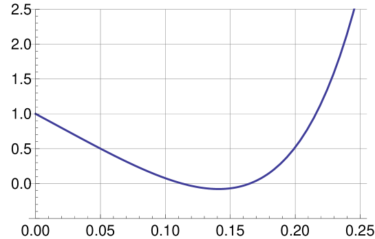
Figure 1. The graph of the Jacobian $J_{F_{0}}(r)$ for $r\in(0,0.25)\,.$

This observation together with Lewy’s theorem gives that (as the Jacobian changes sign), the function $F_{0}(z)$ is not univalent in $|z|<r$ if $r>r_{\mathcal{S}}$ and thus, $r_{\mathcal{S}}$ cannot be replaced by a larger number. $\Box$

Proof of Theorem 1.9. Following the notation and the method of the proof of Theorem 1.5, it suffices to show that $f_{r}\in{\mathcal{C}}_{H}^{2}\cap{\mathcal{S}}_{H}^{*0}$. According to Lemma 2.4, $f_{r}\in{\mathcal{C}}_{H}^{2}\cap{\mathcal{S}}_{H}^{*0}$ whenever $S\leq 1$, where

$$S=\sum_{n=2}^{\infty}n|a_{n}|r^{n-1}+\sum_{n=2}^{\infty}n|b_{n}|r^{n-1}$$

when $a_{n}$ and $b_{n}$ satisfy the coefficient inequalities given by (1.7). Finally, using (1.7), we see that $S\leq 1$ if $r$ satisfies the inequality

$$\sum_{n=2}^{\infty}\frac{n(n+1)}{2}r^{n-1}\leq 1-\sum_{n=2}^{\infty}\frac{n(n-1)}{2}r^{n-1}.$$

The last inequality is easily seen to be equivalent to

$$\frac{1}{2}\left[\frac{1}{(1-r)^{2}}+\frac{1+r}{(1-r)^{3}}-1\right]\leq 1+\frac{1}{2}\left[\frac{1}{(1-r)^{2}}-\frac{1+r}{(1-r)^{3}}-1\right]$$

which upon simplification reduces to

$$2(1-r)^{3}-1-r=-(2r^{3}-6r^{2}+7r-1)\geq 0.$$

The first part of the conclusion easily follows as in the proof of Theorem 1.5.

The sharpness part of the statement of Theorem 1.9 follows if we consider the function

$$L_{0}(z)=2z-M(z)-\overline{N(z)},$$

where $M$ and $N$ are defined by (1.8). We note that

$$L_{0}(z)=z-\sum_{n=2}^{\infty}\frac{n+1}{2}z^{n}+\overline{\sum_{n=2}^{\infty}\frac{n-1}{2}z^{n}}.$$

Again, as $L_{0}$ has real coefficients, we can easily obtain that for $r\in(0,1)$

$$J_{L_{0}}(r) =\left(2-M^{\prime}(r)\right)^{2}-\left(N^{\prime}(r)\right)^{2}$$

$$=\left(2-M^{\prime}(r)+N^{\prime}(r)\right)\left((2-M^{\prime}(r)-N^{\prime}(r)\right)$$

$$=\left(2-\frac{1+r}{(1-r)^{3}}\right)\left(2-\frac{1}{(1-r)^{2}}\right)$$

$$=\frac{2}{(1-r)^{5}}\left(2(1-r)^{3}-(1+r)\right)\left(r-1-\frac{\sqrt{2}}{2}\right)\left(r-1+\frac{\sqrt{2}}{2}\right).$$

We see that $J_{L_{0}}(r_{S})=0$, $0<r<1$ if and only if

$$r=r_{S}\approx 0.16487$$

or

$$r=r^{\prime}_{S}=\frac{2-\sqrt{2}}{2}\approx 0.292893.$$

Moreover for $r_{S}<r<r^{\prime}_{S}$ we have $J_{L_{0}}(r)<0$. The graph of the function $J_{L_{0}}(r)$ for $r\in(0,0.35)$ is shown in Figure 2.

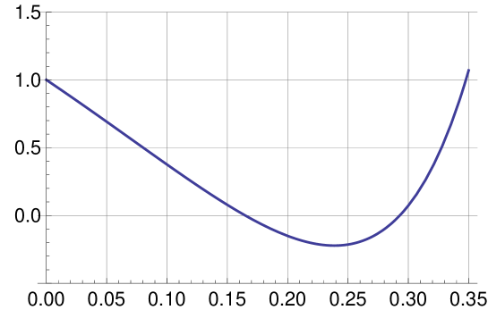
Figure 2. The graph of the Jacobian $J_{L_{0}}(r)$ for $r\in(0,0.35)\,.$

Thus, according to Lewy’s theorem, $L_{0}(z)$ is not univalent in $|z|<r$ if $r>r_{\mathcal{S}}$ and this observation shows that $r_{\mathcal{S}}$ cannot be replaced by a larger number. $\Box$

Proof of Theorem 1.11. This time we apply Lemma 2.1 and show that $f_{r}$ defined by $f_{r}(z):=r^{-1}f(rz)=r^{-1}h(rz)+r^{-1}\overline{g(rz)}$ belongs to ${\mathcal{C}}_{H}^{2}$.

As in the proof of previous two theorems, it suffices to show the corresponding coefficient inequality (2.2), namely,

$$S=\sum_{n=2}^{\infty}n(|a_{n}|+|b_{n}|)r^{n-1}+|b_{1}|\leq 1.$$

By the hypothesis, $|a_{n}|+|b_{n}|\leq c$ for all $n\geq 2$ and so, the last inequality $S\leq 1$ clearly holds if $r$ satisfies the inequality

$$c\left(\frac{1}{(1-r)^{2}}-1\right)\leq 1-|b_{1}|,~{}\mbox{ i.e. }~{}r\leq r_{S}=1-\sqrt{\frac{c}{c+1-|b_{1}|}}.$$

Thus, by Lemma 2.1,

$$|h_{r}^{\prime}(z)-1|<1-|g_{r}^{\prime}(z)|$$

holds for all $z\in{\mathbb{D}}$ whenever $r\leq r_{S}$. Thus, $f\in{\mathcal{C}}_{H}^{2}$.

The function $f_{0}(z)=h_{0}(z)+\overline{g_{0}(z)}$, where

$$h_{0}(z)=z-\frac{c}{2}\left(\frac{z^{2}}{1-z}\right)\textrm{ and }~{}g_{0}(z)=-|b_{1}|z-\frac{c}{2}\left(\frac{z^{2}}{1-z}\right),$$

shows that the result is sharp. Indeed, it is easy to compute that

$$J_{f_{0}}(r)=|h_{0}^{\prime}(r)|^{2}-|g_{0}^{\prime}(r)|^{2}=(1+|b_{1}|)\left(1+c-|b_{1}|-\frac{c}{(1-r)^{2}}\right)$$

which shows that $J_{f_{0}}(r_{S})=0$ and $J_{f_{0}}(r)<0$ for $r>r_{S}$. The proof of the theorem is complete. $\Box$

Proof of Theorem 1.12. Let $f=h+\overline{g}$ be a harmonic mapping defined on the unit disk ${\mathbb{D}}$ with $f(0)=f_{\overline{z}}(0)=f_{z}(0)-1=0$, and $|f(z)|<M$ for $z\in{\mathbb{D}}$, where $h$ and $g$ have the form (1.1) with $b_{1}=0$. According to [4, Lemma 1] (see also [5]), we obtain the sharp estimates

(3.2) $$|a_{n}|+|b_{n}|\leq\frac{4M}{\pi}~{}\mbox{ for any $n\geq 1$}.$$

As $b_{1}=0$ and $a_{1}=1$, it follows that $M\geq\pi/4\approx 0.785398$. By Theorem 1.11 with $c=4M/\pi$, we conclude that $f$ is close-to-convex and starlike (because $b_{1}=0$) for $|z|<1-\sqrt{c/(c+1)}=r_{S}$.

In particular, $f$ is univalent for $|z|<r_{S}$ and furthermore, we have for $|z|=r_{S}$,

$$|f(z)| = \left|z+\sum_{n=2}^{\infty}\big{(}a_{n}z^{n}+\overline{b_{n}z^{n}}\big{)}\right|$$

$$\geq |z|-\left|\sum_{n=2}^{\infty}\big{(}a_{n}z^{n}+\overline{b_{n}z^{n}}\big{)}\right|$$

$$\geq r_{S}-\sum_{n=2}^{\infty}(|a_{n}|+|b_{n}|)r_{S}^{n}$$

$$\geq r_{S}-\frac{4M}{\pi}\sum_{n=2}^{\infty}r_{S}^{n}$$

$$= r_{S}-\frac{4M}{\pi}\frac{r_{S}^{2}}{1-r_{S}}=R_{S}$$

and the proof is complete. $\Box$

References

[1]S. V. Bharanedhar and S. Ponnusamy, Coefficient conditions for
harmonic univalent mappings and hypergeometric mappings,
Preprint
[2]D. Bshouty and A. Lyzzaik, Problems and conjectures in planar harmonic mappings:
in the Proceedings of the ICM2010 Satellite Conference: International Workshop on
Harmonic and Quasiconformal Mappings (HQM2010) (edited by D. Minda, S. Ponnusamy, and N. Shanmugalingam);
Special issue in:
J. Analysis18(2010), 69–82
[3]H. Chen, P. M. Gauthier and W. Hengartner,
Bloch constants for planar harmonic mappings, Proc. Amer.
Math. Soc.128(2000), 3231–3240.
[4]Sh. Chen, S. Ponnusamy and X. Wang,
Bloch and Landau’s theorems for planar -harmonic mappings,
J. Math. Anal. and Appl.373(2011), 102–110.
[5]Sh. Chen, S. Ponnusamy and X. Wang,
Coefficient estimates and Landau-Bloch’s constant for planar
harmonic mappings, Bull. Malaysian Math. Sciences Soc. (2)34(2)(2011), 255–265.
[6]J. G. Clunie and T. Sheil-Small, Harmonic univalent functions,
Ann. Acad. Sci. Fenn. Ser. A.I.9 (1984), 3–25.
[7]M. Dorff and M. Nowak,
Landau’s theorem for planar harmonic mappings, Comput.
Methods Funct. Theory4(2004), 151–158.
[8]P. Duren,Harmonic Mappings in the Plane, Cambridge Tracts in
Mathematics, 156, Cambridge Univ. Press, Cambridge, 2004.
[9]A. Grigoryan,
Landau and Bloch theorems for planar harmonic mappings,
Complex Var. Elliptic Equ.51(2006), 81–87.
[10]H. Lewy,
On the nonvanishing of the Jacobian in certain one-to-one mappings,
Bull. Amer. Math. Soc.42 (1936), 689–692.
[11]M. Sh. Liu,
Landau’s theorem for biharmonic mappings, Complex Var.
Elliptic Equ.9(2008), 843–855.
[12]M. Sh. Liu,
Estimates on Bloch constants for planar harmonic mappings,
Sci. China Ser. A-Math.52(1)(2009), 87–93.
[13]S. Ponnusamy, H. Yamamoto and H. Yanagihara,
Variability Regions for certain families of harmonic univalent
mappings, Complex Var. Elliptic Equ. (2011), To appear.
xxx–xxx.
[14]S. Ruscheweyh and L. Salinas,
On the preservation of direction-convexity and the Goodman-Saff conjecture,
Ann. Acad. Sci. Fenn. Ser. A I Math., 14 (1989), 63–73.
[15]T. Sheil-Small, Constants for planar harmonic mappings,
J. London Math. Soc., 42(1990), 237–248.
[16]H. Silverman,
Univalent functions with negative coefficients, J. Math. Anal. Appl.220(1998), 283–289.
[17]Xiao-Tian Wang and Xiang-Qian Liang,
Precise coefficient estimates for Close-to-convex harmonic univalent mappings,
J. Math. Anal. Appl.263(2001), 501–509.