Multiwavelength campaign on Mrk 509

Abstract

Context. We study the bright Seyfert 1 galaxy Mrk 509 with the Reflection Grating Spectrometers (RGS) of XMM-Newton using the RGS multi-pointing mode of XMM-Newton for the first time in order to constrain the properties of the outflow in this object.

Aims. We want to obtain the most accurate spectral properties from the 600 ks spectrum of Mrk 509 which has excellent statistical quality.

Methods. We derive an accurate relative calibration for the effective area of the RGS, derive an accurate absolute wavelength calibration, improve the method for adding time-dependent spectra and enhance the efficiency of the spectral fitting by two orders of magnitude.

Results. We show the major improvement of the spectral data quality due to the use of the new RGS multi-pointing mode of XMM-Newton. We illustrate the gain in accuracy by showing that with the improved wavelength calibration the two velocity troughs observed in UV spectra are resolved.

1 Introduction

Outflows from Active Galactic Nuclei (AGN) play an important role in the evolution of the super-massive black holes (SMBH) at the centres of the AGN, as well as on the evolution of the host galaxies and their surroundings. In order to better understand the role of photo-ionised outflows, the geometry must be determined. In particular, our goal is to determine the distance of the photo-ionised gas to the SMBH, which currently has large uncertainties. For this reason we have started a large monitoring campaign on one of the brightest AGN with an outflow, the Seyfert 1 galaxy Mrk~509 (Kaastra et al. 2011). The main goal of this campaign is to track the response of the photo-ionised gas to the temporal variations of the ionising X-ray and UV continuum. The response time immediately yields the recombination time scale and hence the density of the gas. Combining this with the ionisation parameter of the gas, the distance of the outflow to the central SMBH can be determined.

The first step in this process is to accurately determine the physical state of the outflow: what is the distribution of gas as a function of ionisation parameter, how many velocity components are present, how large is the turbulent line broadening, etc. Our campaign on Mrk 509 is centred around ten observations with XMM-Newton spanning seven weeks in the Fall of 2009. The properties of the outflow are derived from the high-resolution X-ray spectra taken with the Reflection Grating Spectrometers (RGS, den Herder et al. 2001) of XMM-Newton. The time-averaged RGS spectrum is one of the best spectra ever taken by this instrument, and the statistical quality of this spectrum can be used to improve the current accuracy of the calibration and analysis tools. This gives rise to challenges for the analysis of the data. The methods developed here also apply to other time-variable sources. Therefore we describe them in some detail in this paper.

For this work we have derived a list of the strongest absorption lines in the X-ray spectrum of Mrk 509, and we perform some simple line diagnostics on a few of the most prominent features. The full time-averaged spectrum will be presented elsewhere (Detmers et al. 2011).

2 Data analysis

Table 1: Observation log.

Obs.	ID	Start date	net exposure
nr.			(ks)
1	0601390201	15 Oct 2009	60
2	0601390301	19 Oct 2009	53
3	0601390401	23 Oct 2009	61
4	0601390501	29 Oct 2009	60
5	0601390601	2 Nov 2009	63
6	0601390701	6 Nov 2009	63
7	0601390801	10 Nov 2009	61
8	0601390901	14 Nov 2009	60
9	0601391001	18 Nov 2009	65
10	0601391101	20 Nov 2009	63

Table 1 gives some details on our observations. We quote here only exposure times for RGS. The total net exposure time is 608 ks. No filtering due to enhanced background radiation was needed for these observations, as the background was very low and stable for the full duration of our campaign.

The campaign consisted of ten different observations. Each observation was pointed a bit differently to obtain slightly different positions of the spectra on the detectors (the Multi-Pointing Mode of RGS; steps of 0, $\pm 15^{\prime\prime}$ and $\pm 30^{\prime\prime}$). In this way holes in the detector, due to bad CCD columns and pixels and CCD gaps, changed position over the spectra, allowing all spectral bins to be sampled at some time. In addition this procedure will limit outliers in individual wavelength bins, due to isolated noisy CCD pixels, since the noise of these pixels will be spread over more wavelength bins.

After all exposures were separately processed using the standard RGS pipeline of the XMM-Newton data analysis system SAS version 9, noise due to remaining noisy CCD columns and pixels was decreased further using the following process. Two-dimensional plots of the spectral image (cross-dispersion position versus dispersion angle) and the CCD-pulse height versus spectral dispersion were plotted in the detector reference frame for each separate CCD node, but with all exposures combined. Since spectral features will be smeared out in these plots, possible CCD defects like hot or dead columns and hot or dead pixels are clearly visible. In this way a number of additional bad columns and pixels were manually identified for each detector CCD node and added to the SAS bad pixel calibration file. After this, all exposures were reprocessed, using the new bad pixel tables.

3 Combination of spectra

To obtain an accurate relative effective area and absolute wavelength calibration, we need the signal-to-noise of the combined 600 ks spectrum. Therefore we first describe how to accurately combine the individual spectra, and discuss the effective area and wavelength scale later.

3.1 Combination of spectra from the same RGS and spectral order

Detectors like the RGS yield spectra with lacking counts in parts of the spectrum due to the presence of hot pixels, bad columns or gaps between CCDs. This gives rise to problems when spectra taken at different times have to be combined into a single spectrum, in particular when the source varies in intensity and the lacking counts fall on different wavelengths for each individual spectrum. For RGS this is for example the case when the multi-pointing mode is used like in our present Mrk 509 campaign, or when data of different epochs with slightly different pointings are combined, or if bad columns have (dis)appeared between different observations due to the transient nature of some bad pixels.

Figure 1: Illustration that spectra with different flux and different missing bins cannot be simply added. Both spectrum 1 and 2 have 1 s exposure but have different constant expected count rates of 400 and 200 counts s^-1. In spectrum 1 pixel A is missing, in spectrum 2 pixel B. The thick solid line in the total spectrum indicates the predicted number of counts by straightforwardly adding the response matrices for both spectra with equal weights.

Under the above conditions the SAS task rgscombine should not be used. We illustrate this with a simplified example (Fig. 1). Consider two spectra of the same X-ray source, labelled 1 and 2, with 7 spectral bins each (Fig. 1). The source has a flat spectrum and the flux per bin in spectrum 1 is twice the flux of spectrum 2. In spectrum 1, bin A is missing (zero counts), and in spectrum 2, bin B is missing. The combined spectrum has 600 counts, except for bins A and B with 200 and 400 counts, respectively. However, when the response matrices of both observations are combined, it is assumed that bins A and B were on for 50% of the time, hence the model predicts 300 counts for those bins. Clearly, the data show a deficit or excess at those bins, which an observer could easily misinterpret as an additional astrophysical absorption or emission feature at bins A and B.

How can this problem be solved? One possibility is to fit all spectra simultaneously. However, when there are many different spectra (like the 40 spectra obtained from 2 RGS detectors in two spectral orders for ten observations that we have for our Mrk 509 data), this can be a cumbersome procedure as the memory and CPU requirements become very demanding. Another option is to rigorously discard all wavelength bins where even during short periods (a single observation or a part of an observation) data are lacking. This solution will cause a significant loss of diagnostic capability, as many more bins are discarded and likely several of those bins will be near astrophysically interesting features.

Here we follow a different route. It is common wisdom (and this is also suggested by the SAS manual) not to use fluxed spectra for fitting analysis. The problem is the lack of a well-defined redistribution function for that case. We will show later in Sect. 4 that we can obtain an appropriate response matrix for our case, allowing us to do analysis with fluxed spectra under the conditions given in that section.

We first create individual fluxed spectra using the SAS task rgsfluxer. We use exactly the same wavelength grid for each observation. We then average the fluxed spectra using for each spectral bin the exposure times as weights. This is done for all bins having 100% exposure and for all spectra that are to combined.

For bins with lacking data (like bins A and B of Fig. 1) we have to follow a different approach. If the total exposure time of spectrum $k$ is given by $t_{k}$, and the effective exposure time of spectral bin $j$ in spectrum $k$ is given by $t_{kj}$, we clearly have $t_{kj}<t_{k}$ for “problematic” bins $j$, and we will include in the final spectrum only data bins with $t_{kj}>ft_{k}$, with $0\leq f\leq 1$ a tunable parameter discussed below. However, due to the variability of the source the average flux level of the included spectra $k$ for problematic bin $j$ may differ from the flux level of the neighbouring bins $j-1$ and $j+1$ that are fully exposed. To correct for this, we assume that the spectral shape (but not the overall normalisation) in the local neighbourhood of bin $j$ is constant in time. From these neighbouring bins (with fluxes $F_{j-1}$ and $F_{j+1}$) we estimate the relative contribution $R$ to the total flux for the spectra $k$ that have sufficient exposure time $t_{kj}$ for bin $j$, i.e.

$$R\equiv\frac{\sum\limits_{{k,\ t_{kj}>ft_{k}}}t_{k}F_{j-1}}{\sum\limits_{{k}}t_{k}F_{j-1}},$$ (1)

and similar for the other neighbour at $j+1$. We interpolate the values for $R$ linearly at both sides to obtain a single value at the position of bin $j$. The flux for bin $j$ is now estimated as

$$F_{j}=\frac{\sum\limits_{{k,\ t_{kj}>ft_{k}}}t_{k}F_{j}}{R\ \sum\limits_{{k}}t_{k}}.$$ (2)

Example: for bin $A$ in Fig. 1 we have $R=200\times 1/(400\times 1+200\times 1)=1/3$, and hence using the flux measurement in spectrum 2, we have $F_{A}=(200\times 1)/((1/3)\times 2)=300$ counts s^-1, as it should be.

This procedure gives reliable results as long as the spectral shape does not change locally; as there is less exposure at bin $j$, the error bar on the flux will obviously be larger. However, when there is reason to suspect that the bin is at the location of a spectral line that changes in equivalent width, this procedure cannot be applied!

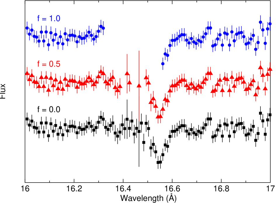
Figure 2: Spectral region near the gap between CCD 5 and 6 of RGS2, containing the 1s–3p line of O viii at 16.55 Å from the outflow. From top to bottom we show the fluxed spectra (arbitrarily scaled and shifted along the flux axis) for three values of $f$. Using the conservative setting $f=1$, a major part of the spectrum is lost. With $f=0$ no data are lost but of course between 16.3 and 16.55 Å the error bars are slightly larger due to the shorter exposure time in that wavelength region.

To give the user more flexibility, we have introduced the minimum exposure fraction $f$ in (1). For $f=0$, we obtain the best results for spectra with constant shape (as every bit of information that is available is used). On the other hand, if $f=1$, only those data bins will be included that have no bad bins in any of the observations to be combined. The advantage in that case is that there is no bias in the stacked spectrum, but a disadvantage is that a significant part of the spectrum may be lost, for example near important diagnostic lines. In particular for the multi-pointing mode the purpose of which is to have different wavelengths fall on different part of the spectrum and thus to have a measurement of the spectrum at all wavelengths, this can be a problem. We illustrate this for the region near the chip gap between CCD 5 and 6 of RGS2 (see Fig. 2). For $f<1$ some data points have large error bars due to the low effective exposure of some bins containing missing columns, and the corresponding low number of counts $N$ yielding large relative errors ($\sim N^{-0.5}$). In our further analysis we use $f=0.$

Finally, in the combined spectrum due to the binning and randomisation procedures within the SAS task rgsfluxer, it is still possible that despite careful screening for bad pixels, a few bad bins remain in the fluxed spectrum, often adjacent or close to discarded bins. For this reason, we check for any bins that are more than $3\sigma$ below their right or left neighbouring bin (taking the statistical errors of both into account). Typically, the algorithm finds a few additional bad bins in an individual observation, which we also discard from our analysis. Only for very strong isolated emission lines with more than 1500 counts in a single observation our method would produce false rejections near the bending points of the instrumental spectral redistribution function, because then the spectral changes for neighbouring bins are stronger than 3$\sigma$ statistical fluctuations, but our spectra of Mrk 509 do not contain such sharp and strong features.

We have implemented the procedures presented in this Section in the program rgs_fluxcombine that is available within the publicly available SPEX distribution.

Finally, we note that in principle another route exists to combine the spectra. This would be to run rgscombine but to modify by a user routine the column AREASCAL so that the count rates are properly corrected for the missing bins. It can be shown that in the combined spectrum AREASCAL must be scaled by $1/R$, with $R$ derived as described above, in order to obtain robust results. It requires however the development of similar tools as rgs_fluxcombine to do this modification.

3.2 Combination of spectra from different RGS or spectral order

In the previous section we showed how to combine spectra from the same RGS and spectral order, but for different observations. However, we also want to combine RGS1 and RGS2 spectra, and spectra from the first and second spectral order. We do this by simply averaging the fluxed spectra, using for each bin the statistical errors on the flux as weight factors. Because of the lower effective area in the second spectral order, second order spectra get in this way less weight then first order spectra, their weights are typically between 20% (near 18 Å) and 50% (near 8 Å) of the first-order spectral weights.

In Sect. 4 we show how to create a response matrix for the fluxed RGS spectra. The same weights that are used to determine the relative contributions of the different spectra to the combined spectrum are also used to weigh the contributions from the corresponding redistribution functions. To avoid discontinuities near the end points of second order spectra or near missing CCDs, we pay attention to small effective area corrections, as outlined in Sect. 5.

4 Response matrix

We have explained before that for time-variable sources standard SAS tasks like rgscombine cannot be used to combine the 10 individual spectra of Mrk 509 or any other source into a single response matrix. For that reason, we have combined fluxed spectra as described in the sections above. The only other feasible alternative would be to fit the 10 individual spectra simultaneously. But with 2 RGS detectors, 2 spectral orders and 10 observations, this adds up to 40 individual spectra. The memory occupied by the corresponding response matrices is 2.0 Gbyte. Although our fitting program SPEX is able to cope with this, fitting becomes cumbersome and error searches extremely slow, due to the large number of matrix multiplications that have to be performed.

For our combined fluxed spectra, fitting is much faster because we have only a single spectrum and hence only need one response matrix. As we use fluxed spectra, we can use a simple response matrix with unity effective area, and the spectral redistribution function given by the redistribution part of the RGS matrix. Unfortunately, the RGS response matrix produced by the SAS rgsrmfgen task combines the effective area and redistribution part into a single data file. Furthermore, due to the multi-pointing mode that we used and due to transient bad columns, the matrix for each of the 10 observations will be slightly different.

Therefore, we have adopted the following approach. For a number of wavelengths (7 to 37 Å, step size 2 Å), we have fitted the RGS response to the sum of three or four Gaussians. This gives a quasi-diagonal matrix resulting in another speed-up of spectral analysis. For these fits to the redistribution function, we have omitted the data channels with incomplete exposure (near chip boundaries, and at bad pixels). The parameters of the Gaussians (normalisation, centre and width) were then modelled with smooth analytical functions of wavelength. We paid most attention to the peak of the redistribution function, where most counts are found.

Table 2: Parameters of the RGS redistribution function.

RGS	RGS1	RGS2	RGS1	RGS2
Order	$-1$	$-1$	$-2$	$-2$
$a_{1}$	0.0211	0.0237	0.0100	0.0118
$a_{2}$	0.0514	0.055	0.018	0.027
$a_{3}$	0.0105	0.016	$-$0.0572	0.017
$a_{4}$	–	–	0.404	0.339
$b_{1}$	0.00028	0.00032	0.00031	0.00035
$b_{2}$	0.00039	0.00058	0.00075	0.00080
$b_{3}$	0.021	0.020	0.021	0.00066
$b_{4}$	–	–	$-$0.01	–
$c_{3}$	$-$0.000405	$-$0.000346	$-$0.000692	–
$d_{2}$	0.1068	0.1314	$-$1.1022	0.0084
$d_{3}$	–	–	1.5276	1.2276
$d_{4}$	–	–	0.3190	$-$0.1211
$e_{2}$	0.0125	0.0086	0.289	0.0153
$e_{3}$	–	–	$-$0.223	$-$0.140
$e_{4}$	–	–	$-$0.017	0.0833
$f_{2}$	$-$0.00024	$-$0.00017	$-$0.0215	$-$0.00024
$f_{3}$	–	–	0.016	0.0075
$f_{4}$	–	–	$-$0.0014	$-$0.0080
$g_{2}$	–	–	0.00053	$-$0.000009
$g_{3}$	–	–	$-$0.00044	$-$0.00015
$g_{4}$	–	–	0.00011	0.00022

The following parametrisation describes the RGS redistribution functions well (all units are in Å):

$$R(\lambda^{\prime},\lambda)=\sum\limits_{i=1}^{4}\frac{N_{i}}{\sqrt{2\pi}\sigma_{i}}\mathrm{e}^{\displaystyle{-(\lambda-\lambda^{\prime})^{2}/2\sigma_{i}^{2}}},$$ (3)

$$\sigma_{i}=a_{i}+b_{i}\lambda+c_{i}\lambda^{2},$$ (4)

$$i=1:\ \ N_{1}=1-N_{2}-N_{3}-N_{4},$$ (5)

$$i=2,\ {\rm 1st\ order\ only:}\ \ N_{i}=d_{i}+e_{i}\lambda+f_{i}\lambda^{2}+g_{i}\lambda^{3},$$ (6)

$$i=2-4,\ {\rm 2nd\ order\ only:}\ \ N_{i}=d_{i}+e_{i}\lambda+f_{i}\lambda^{2}+g_{i}\lambda^{3},$$ (7)

$$i=3,\ {\rm 1st\ order\ RGS1\ only:}\ \ N_{3}=-0.065+2.5/\lambda^{0.7},$$ (8)

$$i=3,\ {\rm 1st\ order\ RGS2\ only:}\ \ N_{3}=-0.075+2.5/\lambda^{0.7}.$$ (9)

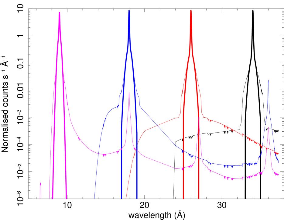
Figure 3: Comparison of the redistribution function for RGS2, first order as delivered by the SAS (thin solid line) to our approximation using three Gaussians (thick lines), for four different photon wavelengths.

Figure 4: As Fig. 3, but only for photons at 18 Å.

The relevant parameters are given in Table 2, omitting parameters that are not used (zero). We cut-off the redistribution function beyond $\pm 1$ Å from the line centre. We have compared these approximations to the true redistribution function (see Figs. 3–4), and find that our model accurately describes the core down to a level of about 1 % of the peak of the redistribution function. Also, the flux outside the $\pm 1$ Å  band is less than $\sim 1$% of the total flux for all wavelengths. It should be noted that the above approximation is more accurate than the calibration of the redistribution itself. Currently, the width of the redistribution is known only to about 10% accuracy.

We finally remark that Fig. 3 seems to suggest that the response also contains the second order spectra, for instance for 9 Å photons, apart from the main peak near 9 Å, there are secondary peaks at 18, 27 and 36 Å. These peaks are, however, not the genuine higher order spectra, but they correspond to higher order photons that by chance end up in the low-energy tail of the CCD redistribution function. For instance, a photon with intrinsic energy 1.38 keV would be seen in first order at 9 Å, but in second order at 18 Å. A small fraction of these second order events end up in the CCD redistribution tail and are not detected near 1.38 keV but near 0.69 keV. Because their (second order) measured wavelength is 18 Å, they are identified as first order events (energy 0.69 keV, wavelength 18 Å). As can be seen from Fig. 3, this is only a small contribution, and we safely can ignore them.

5 Effective area corrections

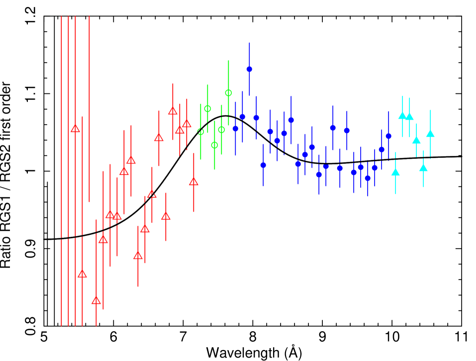
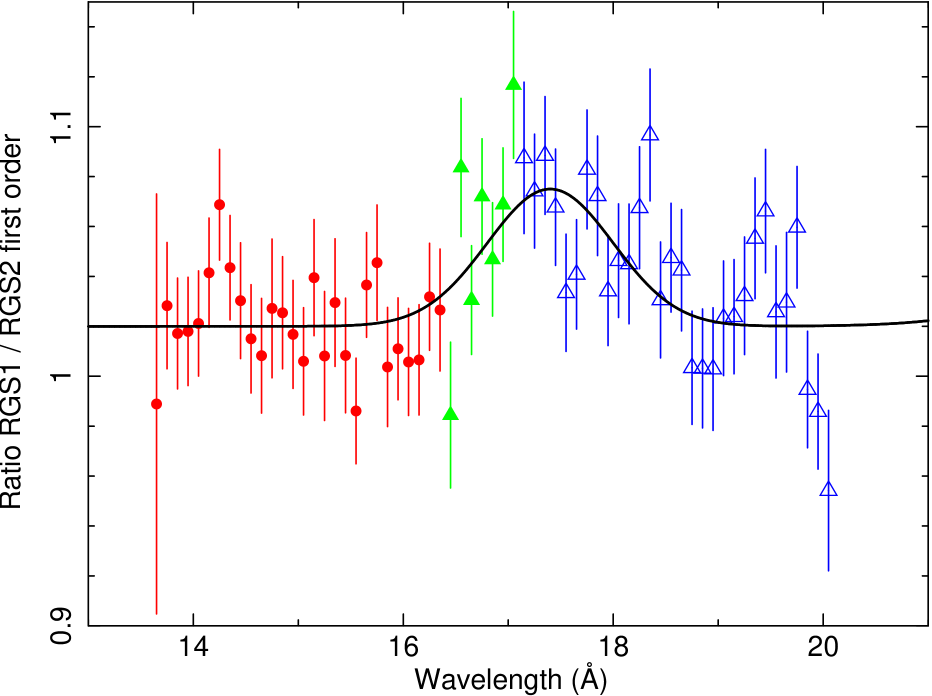
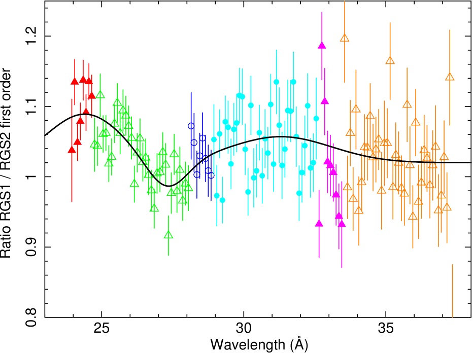
Figure 5: Flux ratio between RGS1 and RGS2 for parts of the spectrum that are detected by both RGS. Different symbols indicate different combinations of CCD chips for both RGS detectors. Open symbols: RGS1 chips 1, 3, 5, 9; filled symbols: RGS1 chips 2, 4, 6, 8. Triangles: RGS2 chips 1, 3, 5, 7, 9; circles: RGS2 chips 2, 6, 8. The solid line is a simple fit to the ratio’s using a constant plus Gaussians.

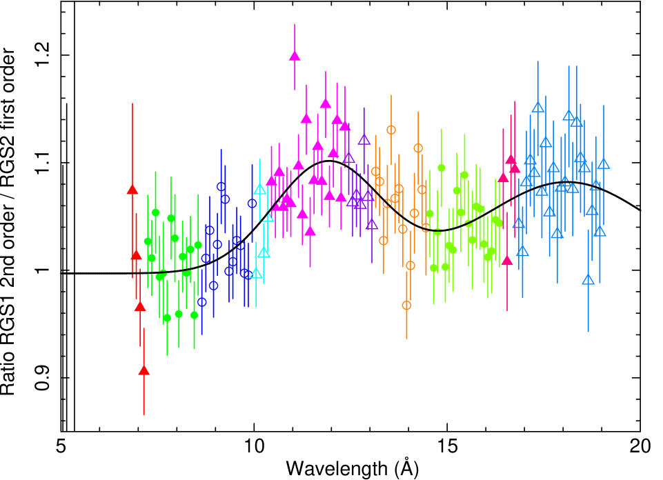
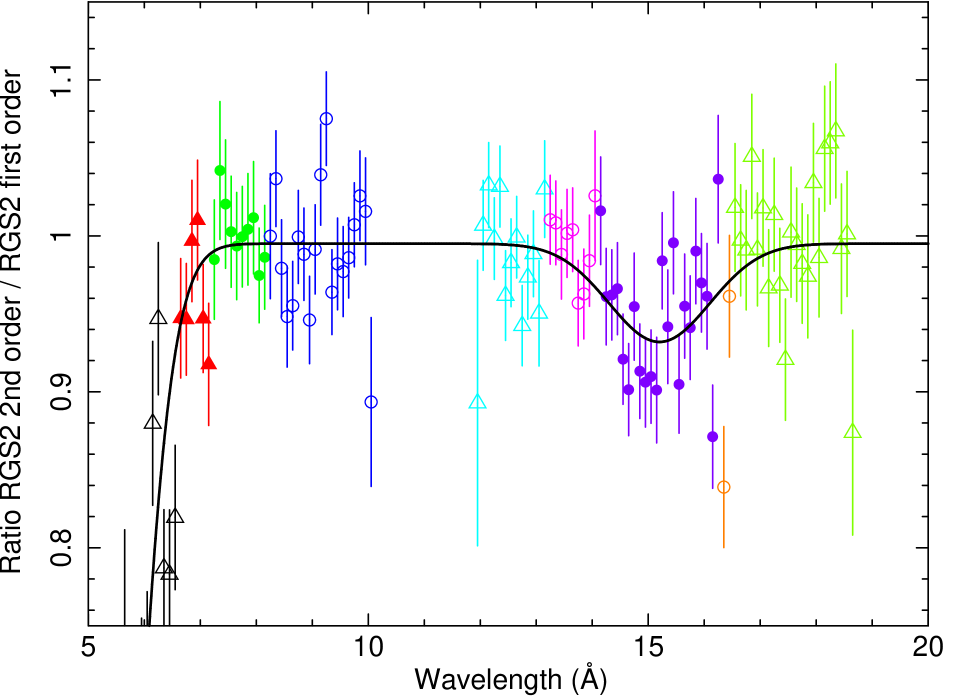
Figure 6: As Fig. 5, but for second order spectra compared to first order spectra. Due to the specific geometry of missing CCDs (CCD7 for RGS1, CCD4 for RGS2) we compare all fluxes to the first order of RGS2. Open symbols: second order chips 1, 3, 5, 7, 9; filled symbols: second order chips 2, 4, 6, 8. Triangles: first order chips 1, 3, 5, 7, 9; circles: first order chips 2, 6, 8.

The statistics of our stacked 600 ks spectrum of Mrk 509 is excellent, with statistical uncertainties down to 2% per 0.1 Å per RGS in first order. In larger bins of 1 Å wide, the quality is even better by a factor of $\sim 3$. These statistical uncertainties are smaller than the accuracy to which the RGS effective area has been calibrated. A close inspection of the first and second order spectra of our source for both RGS detectors showed that there are some systematic flux differences of up to a few percent at wavelength scales larger than a few tenths of an Å (Figs. 5–6), consistent with the known accuracy of the effective area calibration. These differences sometimes correlate with chip boundaries (like at 34.5 Å) but not always. A preliminary analysis shows the same trends for stacked RGS spectra of the blazar Mrk 421.

While a full analysis is underway, we use here a simple approach to correct these differences and obtain an accurate relative effective area calibration. We model the differences purely empirical with the sum of a constant function and a few Gaussians with different centroids, widths and amplitudes, as indicated in Figs. 5–6. We then attribute half of the deviations to RGS1 and the other half to RGS2. In this way there is better agreement between the different RGS spectra, in particular across spectral regions where due to the failure of one of the chips the flux would otherwise show a discontinuity at the boundary between a region with two chips and a region with only one chip. As the effective area of the second order spectra has been calibrated with less accuracy than the first order spectra, we adjust the second order spectrum to match the first order spectrum.

Figure 7: Adopted effective area corrections for RGS1 (solid lines) and RGS2 (dashed lines), in first and second spectral order.

We obtain the following corrections factors:

$$r_{11}(\lambda)=1.02 + G(\lambda,-0.108,5,2)$$ (10)

$$+ G(\lambda,0.099,7.5,0.6)$$

$$+ G(\lambda,0.055,17.4,0.6)$$

$$+ G(\lambda,0.069,24.4,1.3)$$

$$+ G(\lambda,-0.042,27.3,0.7)$$

$$+ G(\lambda,0.037,31.3,1.8),$$

$$r_{12}(\lambda)=0.997 + G(\lambda,0.103,11.9,1.4)$$ (11)

$$+ G(\lambda,0.085,18.1,2.2),$$

$$r_{22}(\lambda)=0.995 + G(\lambda,-0.882,5.0,0.7)$$ (12)

$$+ G(\lambda,-0.063,15.2,0.9),$$

Here $r_{ij}$ is the flux of RGS $i$ order $j$ relative to RGS2 order 1 as shown in Figs. 5–6, and $G(\lambda,N,\mu,\sigma)\equiv N{\rm e}^{\displaystyle{-(\lambda-\mu)^{2}/2\sigma^{2}}}$. With these definitions, the fluxes need to be multiplied by correction factors $a_{ij}$ to get the corrected values as follows:

$$a_{11} = (1+1/r_{11})/2$$ (13)

$$a_{21} = (1+r_{11})/2$$ (14)

$$a_{12} = (1+r_{11})/2r_{12}$$ (15)

$$a_{22} = (1+r_{11})/2r_{22}.$$ (16)

The above approach may fail whenever the small discrepancy between one spectrum and the other is caused by a single RGS, and not by both. Then there will be a systematic error in the derived flux with the same Gaussian shape as used for the correction factors, but with half its amplitude. This is compensated largely, however, by our approach where we fit the true underlying continuum of Mrk 509 by a spline, and in our analysis we make sure that we do not attribute real broad lines to potential effective area corrections. The adopted effective area corrections (the inverse of the $a_{ij}$ factors) are shown in Fig. 7. Note that for wavelength ranges with lacking CCDs the effective area corrections are based on the formal continuation of the above equations, and because of that may differ from unity. However, this is still consistent with the absolute accuracy of the RGS effective area calibration.

6 Wavelength scale

6.1 Aligning both RGS detectors

The zero-point of the RGS wavelength scale has a systematic uncertainty of about 8 mÅ (den Herder et al. 2001). According to the latest insights, this is essentially due to a slight tilting of the grating box due to Solar irradiance on one side of it, which causes small temperature differences and hence inhomogeneous thermal expansion. The thermal expansion changes the incidence angle of the radiation on the gratings and hence the apparent wavelength. The details of this effect are currently under investigation. Due to the varying angle of the satellite with respect to the Sun during an orbit and the finite thermal conductivity time scale of the relevant parts, the precise correction will depend also on the history of the satellite orbit and pointing.

Figure 8: Wavelength difference RGS2 – RGS1 for the 9 strongest lines. The dashed line indicates the weighted average of $6.9\pm 0.7$ mÅ.

As corrections for this effect are still under investigation, we take here an empirical approach. We start with aligning both RGS detectors. We have taken the 9 strongest spectral lines in our Mrk 509 spectrum that can be detected on both RGS detectors, and have determined the difference between the average measured wavelength for both RGS detectors in the combined spectrum. We found that the wavelengths measured with RGS2 are $6.9\pm 0.7$ mÅ larger than the wavelengths measured with RGS1 (Fig. 8).

Therefore, we have re-created the RGS2 spectra by sampling them on a wavelength grid similar to the RGS1 wavelength grid, but shifted by $+6.9$ mÅ. Using this procedure, spectral lines always end up in the same spectral bins. This allows us to stack RGS1 and RGS2 spectra by simply adding up the counts for each spectral bin, without a further need to re-bin the counts when combining both spectra.

After applying this correction, we stacked the spectra of both RGS detectors and compared the first and second order spectra. We found that the second order centroids agree well with the first order centroids (to within an accuracy of 3 mÅ) and therefore did not apply a correction.

6.2 Strongest absorption lines

Figure 9: Fluxed, stacked spectrum of Mrk 509. Only the lines used in Table 3 have been indicated. See Detmers et al. (2011) for a more detailed figure.

Table 3: Strongest absorption lines observed in the spectrum of Mrk 509.

Ion	Trans–	$EW$a	$\lambda_{\mathrm{obs}}$b	$\lambda_{\mathrm{lab}}$c	$v$d	Referencee
	ition	(mÅ)	Å	Å	(km s-1)
Fe xxi	2p–3d	$3.0\pm 0.8$	$12.664\pm 0.008$	$12.2840\pm 0.0020$	$-990\pm 200$	Brown et al. (2002)
Fe xix	2p–3d	$8.5\pm 1.2$	$13.979\pm 0.005$	$13.516\pm 0.005$	$-20\pm 150$	Phillips et al. (1999)
Fe xviii	2p–3d	$5.6\pm 0.8$	$14.680\pm 0.005$	$14.207\pm 0.010$	$-330\pm 230$	Phillips et al. (1999)
Mg xi	1s–2p	$3.6\pm 0.7$	$9.465\pm 0.005$	$9.1688\pm 0.0000$	$-590\pm 150$	Flemberg (1942)
Ne x	1s–2p	$9.8\pm 0.9$	$12.539\pm 0.002$	$12.1346\pm 0.0000$	$-300\pm 40$	Erickson (1977)
Ne ix	1s–3p	$2.5\pm 0.9$	$11.921\pm 0.009$	$11.5440\pm 0.0020$	$-480\pm 240$	Peacock et al. (1969)
Ne ix	1s–2p	$13.2\pm 1.1$	$13.897\pm 0.003$	$13.4470\pm 0.0020$	$-260\pm 70$	Peacock et al. (1969)
Ne viii	1s–2p	$5.6\pm 0.8$	$14.118\pm 0.006$	$13.654\pm 0.005$	$-100\pm 160$	Peacock et al. (1969)
Ne vii	1s–2p	$4.0\pm 0.8$	$14.282\pm 0.006$	$13.8140\pm 0.0010$	$-130\pm 130$	Behar & Netzer (2002)
O viii	1s–5p	$2.4\pm 0.9$	$15.332\pm 0.010$	$14.8205\pm 0.0000$	$+30\pm 190$	Erickson (1977)
O viii	1s–4p	$5.2\pm 0.8$	$15.692\pm 0.006$	$15.1762\pm 0.0000$	$-120\pm 110$	Erickson (1977)
O viii	1s–3p	$13.4\pm 1.2$	$16.546\pm 0.002$	$16.0059\pm 0.0000$	$-190\pm 40$	Erickson (1977)
O viii	1s–2p	$31.8\pm 1.4$	$19.615\pm 0.001$	$18.9689\pm 0.0000$	$-110\pm 20$	Erickson (1977)
O vii	1s–5p	$2.7\pm 0.9$	$18.022\pm 0.013$	$17.3960\pm 0.0020$	$+460\pm 230$	Engström & Litzén (1995)
O vii	1s–4p	$10.3\pm 1.3$	$18.382\pm 0.004$	$17.7683\pm 0.0007$	$+40\pm 60$	Engström & Litzén (1995)
O vii	1s–3p	$14.8\pm 1.0$	$19.265\pm 0.003$	$18.6284\pm 0.0004$	$-70\pm 50$	Engström & Litzén (1995)
O vii	1s–2p	$32.7\pm 2.1$	$22.335\pm 0.002$	$21.6019\pm 0.0003$	$-140\pm 20$	Engström & Litzén (1995)
O vi	1s–2p	$21.2\pm 2.3$	$22.771\pm 0.005$	$22.0194\pm 0.0016$	$-90\pm 70$	Schmidt et al. (2004)
O v	1s–2p	$15.8\pm 2.9$	$23.120\pm 0.005$	$22.3700\pm 0.0100$	$-260\pm 140$	Gu et al. (2005)
N vii	1s–2p	$19.0\pm 2.3$	$25.625\pm 0.004$	$24.7810\pm 0.0000$	$-110\pm 50$	Erickson (1977)
N vi	1s–2p	$23.8\pm 2.8$	$29.773\pm 0.004$	$28.7875\pm 0.0002$	$-70\pm 40$	Engström & Litzén (1995)
N v	1s–2p	$7.6\pm 2.3$	$30.402\pm 0.014$	$29.414\pm 0.004$	$-240\pm 150$	Beiersdorfer et al. (1999)
C vi	1s–4p	$5.7\pm 1.9$	$27.933\pm 0.015$	$26.9898\pm 0.0000$	$+150\pm 160$	Erickson (1977)
C vi	1s–3p	$16.2\pm 2.8$	$29.438\pm 0.007$	$28.4656\pm 0.0000$	$-90\pm 70$	Erickson (1977)
C vi	1s–2p	$49.3\pm 3.0$	$34.890\pm 0.002$	$33.7360\pm 0.0000$	$-70\pm 20$	Erickson (1977)
C v	1s–3p	$17.1\pm 3.2$	$36.174\pm 0.005$	$34.9728\pm 0.0008$	$-30\pm 40$	Edlén & Löfstrand (1970)
Fe xvii G	2p–3d	$2.5\pm 0.8$	$15.021\pm 0.008$	$15.0140\pm 0.0010$	$+160\pm 160$	Brown et al. (1998)
Ne x G	1s–2p	$1.6\pm 0.8$	$12.125\pm 0.010$	$12.1346\pm 0.0000$	$-210\pm 240$	Erickson (1977)
Ne ix G	1s–2p	$4.2\pm 0.9$	$13.454\pm 0.006$	$13.4470\pm 0.0020$	$+180\pm 150$	Peacock et al. (1969)
O viii G	1s–2p	$8.2\pm 1.1$	$18.966\pm 0.005$	$18.9689\pm 0.0000$	$-30\pm 80$	Erickson (1977)
O vii G	1s–3p	$5.7\pm 1.1$	$18.624\pm 0.010$	$18.6284\pm 0.0004$	$-70\pm 170$	Engström & Litzén (1995)
O vii G	1s–2p	$16.6\pm 2.2$	$21.604\pm 0.004$	$21.6019\pm 0.0003$	$+30\pm 50$	Engström & Litzén (1995)
O vi G	1s–2p	$4.5\pm 1.8$	$22.025\pm 0.013$	$22.0194\pm 0.0016$	$+70\pm 180$	Schmidt et al. (2004)
C vi G	1s–2p	$8.8\pm 2.5$	$33.743\pm 0.013$	$33.7360\pm 0.0000$	$+80\pm 170$	Erickson (1977)
O i G	1s–2p	$29.1\pm 2.8$	$23.521\pm 0.003$	$23.5113\pm 0.0018$	$+130\pm 50$	Kaastra et al. (2010)
N i G	1s–2p	$22.2\pm 4.3$	$31.302\pm 0.009$	$31.2857\pm 0.0005$	$+160\pm 80$	Sant’Anna et al. (2000)

• Equivalent width

• Observed wavelength using the nominal SAS wavelength scale for RGS1, with RGS2 wavelengths shifted downwards by 6.9 mÅ.

• Laboratory wavelength (experimental or theoretical) with best estimate of uncertainty

• Outflow velocity; for lines from the AGN relative to the systematic redshift of 0.034397; for lines from the ISM (labelled “G” in the first column) to the LSR velocity scale. Observed errors and errors in the laboratory wavelength have been combined. The velocities are based on the observed wavelengths of column (4) but corrected for the orbital motion of the Earth, and have in addition been adjusted by adding 1.8 mÅ to the observed wavelengths (see Sect. 6.4.6).

• References for the laboratory wavelengths

To facilitate the derivation of the proper wavelength scale, we have compiled a list of the strongest spectral lines that are present in the spectrum of Mrk 509 (Table 3). We have measured the centroids $\lambda_{0}$ and equivalent widths $EW$ of these lines by fitting the fluxed spectra $F(\lambda)$ locally in a 1 Å wide band around the line centre using Gaussian absorption lines, superimposed on a smooth continuum for which we adopted a quadratic function of wavelength. We took care to re-formulate this model in such a way that the equivalent width is a free parameter of the model and not a derived quantity based on the measured continuum or line peak:

$$F(\lambda)=c\Bigl{\{}1+b(\lambda-\lambda_{0})+a(\lambda-\lambda_{0})^{2}-\frac{EW}{\sigma\sqrt{2\pi}}{\mathrm{e}}^{-(\lambda-\lambda_{0})^{2}/2\sigma^{2})}\Bigr{\}}.$$ (17)

As we focus in this paper entirely on absorption lines, we report here $EW$s for absorption lines as positive numbers. Where needed we added additional Gaussians to model the other strong but narrow absorption or emission lines that are present in the same 1 Å wide intervals around the line of interest. The Gaussians include the instrumental broadening. For the strongest 14 lines we could leave the width of the Gaussians a free parameter; for the others we constrained the width to a smooth interpolation of the width from these stronger lines.

For illustration purposes, we show the full fluxed spectrum (after all corrections that we derived in this paper have ben applied) in Fig. 9. A more detailed view of the spectrum including realistic spectral fits is given in paper III of this series (Detmers et al. 2011).

6.3 Doppler shifts and velocity scale

The spectra as delivered by the SAS are not corrected for any Doppler shifts. We have estimated that the time-averaged velocity of the Earth with respect to Mrk 509 is $-29.3$ km s^-1 for the present Mrk 509 data. Because the angle between the lines of sight towards the Sun and Mrk 509 is close to 90° during all our observations, the differences in Doppler shift between the individual observations are always less than 1.0 km s^-1, with an r.m.s. variation of 0.5 km s^-1. Therefore these differences can be ignored (less than 0.1 mÅ for all lines). The orbital velocity of XMM-Newton with respect to Earth is less than 1.2 km s^-1 for all our observations and can also be neglected.

We need a reference frame to determine the outflow velocities of the AGN. For the reference cosmological redshift we choose here $0.034397\pm 0.000040$ (Huchra et al. 1993), as this value is also recommended by the NASA/IPAC Extragalactic database NED, although the precise origin of this number is unclear; Huchra et al. (1993) refer to a private communication to Huchra et al. in 1988.

Because we do not correct the RGS spectra for the orbital motion of the Earth around the Sun, we will instead use an effective redshift of $0.03450\pm 0.00004$ to calculate predicted wavelengths. This effective redshift is simply the combination of the 0.034397 cosmological value with the average $-29.3$ km s^-1 of the motion of the Earth away from Mrk 509.

For Galactic foreground lines it is common practice to use velocities in the Local Standard of Rest (LSR) frame, and we will adhere to that convention for Galactic lines. The conversion from LSR to Heliocentric velocities for Mrk 509 is given by $v_{\mathrm{LSR}}=v_{\mathrm{Helio}}+8.9\,{\mathrm{km}}\,{\mathrm{s}}^{-1}$, cf. Sembach et al. (1999).

6.4 Absolute wavelength scale

The correction that we derived in Sect. 6.1 aligns both RGS detectors and spectral orders, but there is still an uncertainty (wavelength offset) in the absolute wavelength scale of RGS1. We estimate here this offset by comparing measured line centroids in our spectrum to predicted wavelengths based on other X-ray, UV or optical spectroscopy of Mrk 509. We consider here five different methods:

1. Lines from the outflow of Mrk 509

2. Lines from foreground neutral gas absorption

3. Lines from foreground hot gas absorption

4. Comparison with a sample of RGS spectra of stars

5. Comparison with Chandra LETGS spectra

6.4.1 Lines from the outflow of Mrk 509

The outflow of Mrk 509 has been studied in the past using high-resolution UV spectroscopy with FUSE (Kriss et al. 2000) and HST/STIS (Kraemer et al. 2003). A preliminary study of the COS spectra taken simultaneously with the Chandra LETGS spectra in December 2009, within a month from the present XMM-Newton observations, shows that there are no major changes in the structure of the outflow as seen through the UV lines. Hence, we take the archival FUSE and STIS data as templates for the X-ray lines. Kriss et al. (2000) showed the presence of seven velocity components labelled 1–7 from high to low outflow velocity. Component 4 may have sub-structure (Kraemer et al. 2003) but we ignore here these small differences. The outflow components form two distinct troughs, a high velocity component from the overlapping components 1–3 and a low velocity component from the overlapping components 4–7.

Table 4: Outflow velocities in km s^-1 derived from UV lines.

Feature	$\log\xi$a	Comp	Comp	Comp	wb	Refc
		1–3	4–7	1–7
H i $\lambda 1026$		$-317$	$+6$	$-56$	N	FUSE
H i $\lambda 1026$		$-330$	$+48$	$-89$	EW	FUSE
O vi $\lambda 1032/38$	$+0.4$	$-329$	$+44$	$-28$	N	FUSE
O vi $\lambda 1032/38$		$-338$	$+64$	$-78$	EW	FUSE
N v $\lambda 1239/43$	$-0.1$	$-344$	$+21$	$-166$	N	STIS
C iv$\lambda 1548/51$	$-0.6$	$-328$	$+1$	$-197$	N	STIS
C iii $\lambda 977.02$	$-1.4$	$-347$	$-16$	$-224$	N	FUSE
C iii $\lambda 977.02$		$-339$	$-27$	$-231$	EW	FUSE

• ionisation parameter in $10^{-9}$ W m

• N: weighted average using column densities; EW: weighted average using equivalent widths

• FUSE: Kriss et al. (2000), STIS: Kraemer et al. (2003)

Note that our analysis of ISM lines in the HST/COS spectra for our campaign (Kriss et al. 2011) shows that the wavelength scale for the FUSE data (Kriss et al. 2000) needs a slight adjustment. As a consequence, we subtract 26 km s^-1 from the velocities reported by Kriss et al. (2000), in addition to the correction to a different host galaxy redshift scale.

In Table 4 we list the column density weighted or equivalent width weighted average velocities. We also give the typical ionisation parameter $\xi$ for which the ion has its peak concentration, based upon the analysis of archival XMM-Newton data of Mrk 509 by Detmers et al. (2010).

In principle, equivalent-width weighted line centroids are preferred to predict the centroids of the unresolved X-ray lines. As for most of the X-ray lines the optical depths are not very large, using just the column density weighted average will not make much difference, however.

Table 5: Wavelength differences (observed minus predicted, in mÅ) for selected X-ray lines of the outflow.

Line	$\log\xi^{\mathrm{a}}$	$v^{\mathrm{b}}$	$\Delta v^{\mathrm{c}}$	$\lambda_{\mathrm{obs}}-\lambda_{\mathrm{pred}}$d
		(km s-1)	(km s-1)	mÅ
N vi $\lambda 28.79$	$+0.7$	$-28$	$50$	$-5\pm 7$
O vi $\lambda 22.02$	$+0.4$	$-28$	$10$	$-6\pm 5$
C v $\lambda 34.97$	$+0.1$	$-110$	$100$	$+8\pm 13$
O v $\lambda 22.37$	$0.0$	$-138$	$40$	$-11\pm 12$
N v $\lambda 29.41$	$-0.1$	$-166$	$10$	$-10\pm 15$
average				$-5.3\pm 3.6$

• ionisation parameter in $10^{-9}$ W m

• adopted velocity based on UV lines

• adopted systematic uncertainty in velocity based on the differences in centroids for the UV lines

• statistical uncertainty observed line centroid, uncertainty in laboratory wavelength (Table 3) and the adopted systematic uncertainty in velocity have been added in quadrature

The strong variation of average outflow velocity as a function of $\xi$ that is apparent in Table 4, in particular between O vi and N v, shows that caution must be taken. Therefore, we consider here only X-ray lines from ions which overlap in ionisation parameter with the ions in Table 4. We list those lines in Table 5. For C v and O v we have interpolated the velocity between the O vi and N v velocity according to their $\log\xi$ value. The weighted average shift $\Delta\lambda\equiv\lambda_{\mathrm{obs}}-\lambda_{\mathrm{pred}}$ is $-5.3\pm 3.6$ mÅ.

6.4.2 Lines from foreground neutral gas absorption

Our spectrum (see Table 3) contains lines from the neutral as well as the hot phase of the ISM. Here we discuss the neutral phase. The spectrum shows two strong lines from this phase, the O i and N i is–2p lines. Other lines are too weak to be used for wavelength calibration purposes.

The sight line to Mrk 509 is dominated by neutral material at LSR velocities of about $+10$ km s^-1 and $+60$ km s^-1, as seen for instance in the Na i D₁ and D₂ lines, and the Ca ii H and K lines (York et al. 1982). Detailed 21 cm observations (McGee & Newton 1986) show four components: two almost equal components at $-6$ and $+7$ km s^-1, a weaker component (6% of the total H i column density) at $+59$ km s^-1 and the weakest component at $+93$ km s^-1 containing 0.7% of the total column density.

The strongest X-ray absorption line from the neutral phase is the O i 1s–2p transition. The rest-frame wavelength of this line has been determined as $23.5113\pm 0.0018$ Å (Kaastra et al. 2010). Based on the velocity components of McGee & Newton (1986), we have estimated the average velocity for this line as well as the UV line at 1302 Å, assuming an oxygen abundance of $5.75\times 10^{-4}$ (proto-Solar value: Lodders 2003), adopting that $\sim 50$% of all neutral oxygen is in its atomic form. We predict for the $\lambda$23.5 Å line an LSR velocity of $+24$ km s^-1, and for the $\lambda$1302 Å line a velocity of $+40$ km s^-1. For a two times higher column density, these lines shift by no more than $+6$ and $+1$ km s^-1, respectively. For comparison, the measured centroid of the $\lambda$1302 Å line (Collins et al. 2004, Fig. 6) is $+40$ km s^-1, in close agreement with the prediction. A systematic uncertainty of $\pm 10$ km s^-1 on the predicted $\lambda$23.5 Å line seems therefore to be justified. Taking this into account, we expect the O i line at $23.515\pm 0.002$ Å.

Table 6: Wavelengths (Å) of the O iv 1s–2p transitions; all transitions are from the ground state to 1s2s²2p².

2D3/2	2P1/2	2P3/2	2S1/2	reference
22.777	22.729	22.727	22.571	HULLACa
22.755	22.739	22.736	22.573	Cowan codeb
22.77	22.74	22.74	22.66	AS2 (Autostructure)c
22.78	22.75	22.75	22.65	HF1 (Cowan code)c
22.73	22.67		22.46	R-matrixd
–	22.741$\pm$0.004		–	experimente
22.777	22.741	22.739	22.571	Adopted value
0.010	0.004	0.004	0.025	Adopted uncertainty

• E. Behar 2001, private communication

• A.J.J. Raassen 2001, private communication

• García et al. (2005)

• Pradhan et al. (2003)

• Gu et al. (2005)

Unfortunately, the Galactic O i $\lambda$23.5 Å line is blended by absorption from lines of two other ions in the outflow of Mrk 509, O iv and Ca xv. We discuss those lines below.

Contamination by O iv:

The O iv 1s–2p ²P transition, which has a laboratory wavelength of $22.741\pm 0.004$ Å (Gu et al. 2005), contaminates the Galactic O i line. In fact, the situation is more complex, as the main O iv 1s–2p multiplet has four transitions. In Table 6 we summarise the theoretical calculations and experimental measurements of the wavelengths of these lines. The adopted values are based on the single experimental measurement and the HULLAC calculations, while the adopted uncertainties are based on the scatter in the wavelength differences.

In the present case, both the O iv 1s–2p ²D_3/2 and 1s–2p ²P_1/2 and ²P_3/2 transitions of the outflow blend with the Galactic O i line, with relative contributions of 37, 42 and 21%, respectively. The precise contamination is hard to determine, as these are the strongest O iv transitions and the other O iv transitions are too weak to determine the column density. Based on the absorption measure distribution of other ions with similar ionisation parameter, we estimate that the total equivalent width of these three O iv lines is $3.6\pm 2.0$ mÅ (Detmers et al. 2011). The same modelling predicts that the O iv concentration peaks at $\log\xi=-0.6$, at almost the same ionisation parameter as for C iv. The optical depths of all X-ray lines of O iv is less than 0.1, hence we use the column density weighted average line centroid of C iv ($-197$ km s^-1) for O iv. With this, we predict a wavelength for the combined ²D and ²P transitions of O iv of $23.523\pm 0.004$ Å.

Contamination by Ca xv:

The other contaminant to the Galactic O i 1s–2p line is the Ca xv 2p–3d (³P₀ – ³D₁) $\lambda 22.730$ Å transition of the outflow. This is the strongest X-ray absorption line for this ion. Based on the measured column density of Ca xiv in the outflow, and assuming that the Ca xv column density is similar, we expect an equivalent width of $4.9\pm 2.3$ mÅ for this line, about 10 % of the strength of the O i blend.

The rest-wavelength of this transition is somewhat uncertain, however. Kelly (1987) gives a value of 22.725 Å, without errors, and refers to Bromage & Fawcett (1977) who state that their theoretical wavelength is within 5 mÅ from the observed value of 22.730 Å, and that the line is blended. Although not explicitly mentioned, their experimental value comes from Kelly & Palumbo (1973) (cited in the Bromage & Fawcett paper). Kelly & Palumbo (1973) gives a value of 22.73 Å, but states it is for the ³P₂ – ³D₃ transition, which is a misclassification according to Fawcett & Hayes (1975). They list as their source Fawcett (1971). The latter publication gives the value of 22.73, but no accuracy. In Fawcett (1970) the typical accuracy of the plasma measurements is limited by Doppler motions of about $10^{-4}c$. If we assume that accuracy also holds for the data in Fawcett (1971), the estimated accuracy should be about 2 mÅ. Given the rounding of Fawcett (1970), an r.m.s. uncertainty of 3 mÅ is more appropriate. However, there is some level of blending with other multiplets. Blending is probably due to other 2p–3d transitions in this ion, most likely transitions between the ³P–³D, ³P–³P and ¹D–¹F multiplets (Aggarwal & Keenan 2003). A comparison of the theoretical wavelengths of Aggarwal & Keenan (2003) with the experimental values of Kelly (1987) for all lines of the ³P – ³D multiplet shows, apart from an offset of 145 mÅ, a scatter of 6 mÅ.

Given all this, we adopt here the original measurement of Fawcett (1971), but with a systematic uncertainty of 5 mÅ. As Ca xv has a relatively large ionisation parameter ($\log\xi=2.5$), we expect that like other highly ionised species in Mrk 509 it is dominated by the high-velocity outflow components, that have a velocity of about $-340$ km s^-1 (see Table 4). Putting a conservative $200$ km s^-1 uncertainty on this (allowing a centroid up to halfway between the two main absorption troughs), we may expect the line at $23.488\pm 0.017$ Å.

Centroid of the O i blend:

The total equivalent width of the O i blend is $29.1\pm 2.8$ mÅ (see Table 3). The velocity dispersion of the contaminating O iv and Ca xv lines is an order of magnitude larger than the small velocity dispersion of the cold Galactic gas, and both contaminants have optical depth smaller than unity. The total blend is thus the combination of broad and shallow contaminants with deep and narrow O i components. Thus the contribution due to O i itself is obtained by simply subtracting the contributions from O iv and Ca xv from the total measured equivalent width of the blend. This yields an O i equivalent width of $20.6\pm 4.2$ mÅ. Taking into account the contribution of the contaminants, we expect the centroid of the blend to be at $23.5115\pm 0.0032$ Å. This corresponds to an offset $\Delta\lambda=9.9\pm 4.5$ mÅ.

N i:

The other strong X-ray absorption line from the neutral phase of the ISM is the N i 1s–2p line. We adopt the same LSR velocity as for the unblended O i line, $+24$ km s^-1. This is consistent with the measured line profile of the N i $\lambda 1199.55$ Å line, which shows two troughs at about 0 and $+50$ km s^-1 (Collins et al. 2004). The shift derived from the N i line is therefore $+12.2\pm 8.9$ mÅ.

We note, however, that for N i we can only use RGS2, as RGS1 shows some instrumental residuals near this line. The nominal wavelength for RGS1 is 26 mÅ higher than for RGS2. It is therefore worthwhile to do a sanity check. Therefore we have determined the same numbers from archival data of Sco X-1. That source was observed several times with significant offsets in the dispersion direction, so that the spectral lines fall on different parts of the CCDs or even on different CCD chips. We measure wavelengths for O i and N i in Sco X-1 of $23.5123\pm 0.0015$ and $31.2897\pm 0.0030$ Å, respectively. Sco X-1 has a Heliocentric velocity of $-114$ km s^-1 (Steeghs & Casares 2002). Given its Galactic longitude of 0$\aas@@fstack{\circ}$7, we expect the local foreground gas to have negligible velocity. This is confirmed by an archival HST/GHRS spectrum, taken from the HST/MAST archive, and showing a velocity consistent with zero, to within $5$ km s^-1 for the N i $\lambda 1199.55$ Å line from the ISM. This then leads to consistent observed offsets for the 1s–2p transitions of O i and N i in Sco X-1 of $1.0\pm 2.3$ mÅ and $4.0\pm 3.0$ mÅ, respectively.

Combining both the O i and the N i line for Mrk 509, we obtain a shift of $+10.3\pm 4.0$ mÅ.

6.4.3 Lines from foreground hot gas absorption

Table 7: Decomposition of the O vi profile of Sembach et al. (2003) into Gaussian components.

nr	vLSR	$\sigma$	column
	(km s-1)	(km s-1)	($10^{16}$ m-2)
1	$-$245	59	214
2	$-$126	16	23
3	$-$64	13	19
4	$+$26	44	440
5	$+$152	24	26

Our spectrum also contains significant lines from hot, ionised gas along the line of sight, in particular from O vi, O vii, O viii, and C vi. Sembach et al. (2003) give a plot of the O vi line profile. This line shows clear high-velocity components at $-247$ and $-143$ km s^-1. Unfortunately, no column density of the main Galactic component is given by Sembach et al. (2003). Therefore we have fitted their profile to the sum of 5 Gaussians (Table 7). The column-density weighted centroid for the full line is at $-56$ km s^-1 in the LSR frame. We estimate an uncertainty of about 8 km s^-1 on this number.

Note that a part of the high-velocity trough in the blue is contaminated by a molecular hydrogen line at 1031.19 Å, which falls at $v_{\rm{LSR}}=-206$ km s^-1. This biases component 1 of our fit for the hot foreground galactic component by about 10 km s^-1. This component in C iv, Si iv, and N v in the COS spectra is at a velocity of $v_{\rm{LSR}}=-245$ km s^-1 (Kriss et al. 2011), and therefore we adopt that value here.

Table 8: Line shifts $\Delta\lambda\equiv\lambda_{\mathrm{obs}}-\lambda_{\mathrm{pred}}$ in mÅ for the X-ray absorption lines from the hot interstellar medium.

transition	$\Delta\lambda$a	$\Delta\lambda$b	errorc	errord
	(mÅ)	(mÅ)	(mÅ)	(mÅ)
Fe xvii 2p–3d	9	5	8	13
Ne x 1s–2p	$-$8	$-$11	10	13
Ne ix 1s–2p	9	6	7	11
O vii 1s–3p	$-$3	$-$8	10	16
O viii 1s–2p	0	$-$5	5	14
O vii 1s–2p	$-2$	$-$8	5	15
O vi 1s–2p	8	2	13	13
C vi 1s–2p	11	1	13	26

• Using $v_{\mathrm{L}SR}=-56$ km s^-1

• Using $v_{\mathrm{L}SR}=+26$ km s^-1

• Only statistical error

• Including uncertainty of $\pm 200$ km s^-1 except for O vi

While this velocity can be readily used for predicting the observed wavelength of the O vi 1s–2p line, the uncertainty for other X-ray lines is larger, because the temperatures or ionisation states of the dominant components 1 and 4 may be different. Moreover, O vi is the most highly ionised ion available in the UV band, while most of our X-ray lines from the ISM have a higher degree of ionisation. Therefore, without detailed modelling of all these components, we conservatively assume here for all ions other than O vi an error of 200 km s^-1 on the average outflow, corresponding to the extreme cases that the bulk of the column density is in either component 1 or 5.

The Galactic O vii 1s–2p line at 21.6 Å suffers from some blending by the N vii 1s–3p line from the outflow. That last line, with a predicted equivalent width of 4.5 mÅ, has a relatively high ionisation parameter, $\log\xi=1.4$. Therefore we do not know exactly what its predicted velocity should be, and we conservatively assume a value of $-100\pm 200$ km s^-1, spanning the full range of outflow velocities. With that, the predicted wavelength of the N vii outflow line is $21.624\pm 0.014$ Å, while the predicted wavelength of the O vii line is $21.5993\pm 0.0006$ Å. The predicted wavelength of the blend then is $21.606\pm 0.004$ Å.

In Table 8 we list the lines that we use and the derived line shifts $\Delta\lambda$. The weighted average is $+1.7\pm 2.6$ mÅ when we only include statistical errors, and $+2.8\pm 4.9$  mÅ if we include the systematic uncertainties.

We make here a final remark. Combining all wavelength scale indicators including the one above (Sect. 6.4.6), we obtain an average shift of $-1.6$ mÅ. Using this number, the most significant lines of Table 8 (O vii and O viii 1s–2p) show clearly a velocity much closer to the dominant velocity component 4 ($+26$ km s^-1, Table 7) than to the column-density weighted velocity of the O vi line at $-56$ km s^-1. This last number is significantly affected by the high-velocity clouds, that apparently are less important for the more highly ionised ions. Therefore, in Table 8 we also list in column 3 the wavelength shifts under the assumption that all lines except O vi are dominated by component 4. With that assumption, and taking now only the statistical errors into account, the weighted average shift is $-1.7\pm 2.8$ mÅ.

6.4.4 Comparison with a sample of RGS spectra of stars

Preliminary analysis (R. González-Riestra, private communication) of a large sample of RGS spectra of stellar coronae indicate that there is a correlation between the wavelength offsets and the Solar Aspect Angle (SAA) of the satellite (correlation coefficient about 0.6). At a mean SAA of 90°, the average $\Delta\lambda$ for RGS1 is 2.3 mÅ, while for RGS2 it is 7.3 mÅ. The scatter for an individual observation is 6 and 7 mÅ, respectively. The difference between RGS1 and RGS2 is fairly consistent with the $6.9\pm 0.7$ mÅ that we adopted for the present work. As our observation campaign on Mrk 509 spans the full visibility window, the average SAA angle is 90°; it varied between 108$\aas@@fstack{\circ}$5 for the first observation, to 73$\aas@@fstack{\circ}$3 for the last observation. The wavelengths in our spectrum (averages of the original RGS1 wavelengths and the RGS2 wavelengths minus 6.9 mÅ) should then be off by $+1.4\pm 6.5$ mÅ.

The above estimate can be refined further. It appears that there is also a correlation of the wavelength offset with the temperature parameters T2007 and T2031 of the grating boxes on RGS1 and RGS2, respectively. However, these temperatures do not correlate well with the SAA. Hence, following R. González-Riestra et al. (private communication) and using their data on 38 spectra of stellar coronae, we obtain the following correlations:

$$\mathrm{RGS1}:\ \Delta\lambda=4.92 - 0.49(\mathrm{SAA}-90\degr)$$ (18)

$$- 12.8(\mathrm{T2007}-20.7),$$

$$\mathrm{RGS2}:\ \Delta\lambda=8.32 - 0.55(\mathrm{SAA}-90\degr)$$ (19)

$$- 11.8(\mathrm{T2031}-20.7),$$

where SAA is expressed in degrees, and the temperatures in °C. The scatter around this relation is 4.1 and 4.8 mÅ for RGS1 and RGS2, respectively. This scatter is significantly smaller than the scatter using only the correlation with SAA mentioned above.

Table 9: Average line shifts for the six strongest lines, relative to the total spectrum.

Obs	$\lambda-\overline{\lambda}$a	SAA	T2007	T2031	$\lambda-\overline{\lambda}$b
	(mÅ)	(°)	(oC)	(oC)	(mÅ)
1	$-6.2\pm 3.0$	108.5	21.38	21.48	-10.60
2	$-12.2\pm 2.9$	104.1	21.26	21.38	-6.97
3	$+3.9\pm 1.9$	100.7	21.32	21.42	-5.80
4	$+2.4\pm 2.2$	94.7	21.24	21.33	-1.68
5	$-3.6\pm 2.1$	90.9	21.43	21.51	-1.98
6	$-3.0\pm 2.1$	86.7	21.51	21.54	-0.48
7	$0.0\pm 2.3$	82.7	21.28	21.40	3.90
8	$+7.3\pm 2.3$	78.7	21.32	21.43	5.52
9	$+7.6\pm 2.1$	75.0	21.24	21.35	8.42
10	$+0.3\pm 2.3$	72.7	21.24	21.34	9.68
allc	$\equiv 0$	89.5	21.32	21.42	$\equiv 0$

• Observed wavelength difference for individual observations.

• Predicted wavelength difference for individual observations using (18)–(19); results for RGS1 and RGS2 have been weighted averaged (not all lines present in each RGS).

• Combined spectrum.

Figure 10: Top panel: wavelength difference for the six strongest lines in each observation relative to the lines in the average spectrum (data points) and model based on Eq. (18)–19 (histogram). Bottom panel: residuals of the data points relative to the model in the upper panel.

We apply this now to the 10 individual observations of Mrk 509. We have determined the individual line centroids of the 6 strongest lines (C vi 1s–2p, O viii 1s–2p and 1s–3p, O vii 1s–2p, Ne ix 1s–2p all from the outflow, and O i 1s–2p from the foreground). We then take the difference with the wavelength in the combined observation, and averaged these residuals. We show the results in Table 9 and Fig. 10.

The model gives an improvement: the r.m.s. residuals (after correction for the mean statistical errors on the data points of 2.3 mÅ) are reduced from 5.4 to 4.6 mÅ. This is fully consistent with the remaining residuals in the set of coronal spectra discussed above. It is also clear that the remaining residuals are non-statistical, and although on average the model gives an improvement, in some individual cases the opposite is true, for instance for observations 3, 7 and 10.

Keeping this in mind, we can use the model to predict the absolute wavelength scale. We predict absolute offsets $\Delta\lambda$ of $-2.76$ and $+0.10$ mÅ for RGS1 and RGS2, respectively. In our extraction procedure, we have subtracted 6.9 mÅ from the RGS2 wavelengths; doing the same for the predicted RGS offset, and averaging the offsets for RGS1 and RGS2, the model predicts a total offset of $-4.8$ mÅ. We only need to apply a small correction for the velocity of the Earth. It can be assumed that the sample of stars has, on average, zero redshift due to the motion of Earth, because usually each source can be observed twice a year with opposite signs of the Doppler shift. Our data of Mrk 509 were taken with a rather extreme Earth velocity of $-29.3$ km s^-1. At a typical wavelength of 20 Å, this corresponds to a correction factor of 2.0 mÅ. We finally obtain a predicted offset of $-2.8\pm 4.5$ mÅ  where the error is the average systematic residual found for the sample of coronae mentioned before.

6.4.5 Comparison with Chandra LETGS spectra

Table 10: Comparison of measured wavelengths from the RGS and LETGS.

transition	RGS	LETGS	RGS $-$ LETGS
	(Å)	(Å)	(mÅ)
O viii 1s–3p	$16.5460\pm 0.0023$	$16.552\pm 0.004$	$-6\pm 5$
O vii 1s–3p	$19.2649\pm 0.0029$	$19.269\pm 0.007$	$-4\pm 8$
O viii 1s–2p	$19.6146\pm 0.0012$	$19.619\pm 0.004$	$-4\pm 4$
O vii 1s–2p	$22.3354\pm 0.0018$	$22.346\pm 0.004$	$-11\pm 4$

We have also measured the wavelengths of the 1s–2p and 1s–3p lines of O vii and O viii in the Chandra LETGS spectrum of Mrk 509 taken 20 days after our last XMM-Newton observation. LETGS has the advantage above RGS that it measures both positive and negative spectral orders, hence allow to determine the zero-point of the wavelength scale more accurately. Table 10 lists the wavelengths measured by both instruments. The average wavelength offset of RGS relative to LETGS is $-6.9\pm 2.4$ mÅ. The above number only includes the statistical uncertainties. We have extracted an LETGS spectrum of Capella, taken around the same time as the Mrk 509 observation. The ten strongest lines in the spectrum of Capella between 8–34 Å show a scatter with r.m.s. amplitude of 6 mÅ compared to the laboratory wavelengths, but no systematic offset larger than 2 mÅ. We therefore add a systematic uncertainty of $6/\sqrt{4}=3$ mÅ in quadrature to the statistical uncertainty of the average $\Delta\lambda$ for the four lines in Mrk 509 that we use here.

We only need to make a small correction of $-0.4$ mÅ corresponding to the higher speed of Earth away from Mrk 509 ($-29.3$ km s^-1) during the XMM-Newton observation as compared to the Chandra observation ($-23.3$ km s^-1). This all leads to an offset of $-7.3\pm 3.8$ mÅ.

6.4.6 Summary of results on the wavelength scale

Table 11: Overview of wavelength scale indicators.

Indicator	$\Delta\lambda\equiv\lambda_{\mathrm{obs}}-\lambda_{\mathrm{pred}}$
	(mÅ)
1. Lines from the outflow of Mrk 509	$-5.3\pm 3.6$
2. Lines from foreground neutral gasa	$+10.3\pm 4.0$
2. Lines from foreground neutral gasb	$+6.5\pm 3.4$
3. Lines from foreground hot gas absorptionc	$+2.8\pm 4.9$
3. Lines from foreground hot gas absorptiond	$-1.9\pm 4.9$
4. Comparison with a sample of RGS spectra of stars	$-2.8\pm 4.5$
5. Comparison with Chandra LETGS spectra	$-7.3\pm 3.8$
All indicators combineda,c	$-1.0\pm 1.8$
All indicators combinedb,c	$-1.2\pm 1.8$
All indicators combineda,d	$-1.6\pm 1.8$
All indicators combinedb,d	$-1.8\pm 1.8$

• As described in Sect. 6.4.2

• Ignoring the blending by Ca xv of the O i line

• Using the O vi centroid velocity

• Using the velocity of dominant component 4 in O vi

We now summarise our findings from the previous sections (Table 11). All estimates agree within the error bars, except for the lines from the neutral foreground gas, which is off by about 3$\sigma$. This number is dominated by the rather complex O i blend. Possibly there are larger systematic uncertainties on this number than we assumed. The major factor here is the blending with Ca xv. If we assume that the equivalent width of the contaminating Ca xv line is zero, the predicted blend centroid decreases by 4.4 mÅ, towards better agreement with the other indicators. The O iv blend has a much smaller impact, as its centroid is already close to the centroid of the Galactic O i line.

We note that a smaller value of the predicted equivalent width of the Ca xv line may be caused by a somewhat lower Ca abundance; alternatively, if the density is higher than about $10^{16}$ m^-3, the population of Ca xv in the ground state decreases significantly (Bhatia & Doschek 1993), leading also to a reduced equivalent width of this absorption line.

All five methods used here have their pros and cons, and we have done the best we can to estimate the uncertainties for each of the methods. The five methods are for the major part statistically independent, and this allows us to use a weighted average for the final wavelength correction. Ignoring the blending by Ca xv to the Galactic O i line, and using $+26$ km s^-1 for the outflow velocity of the hot Galactic gas, this wavelength shift is $-1.8\pm 1.8$ mÅ. Within their statistical uncertainties, all individual indicators are consistent with this value, except for the lines from foreground neutral gas, which are off by $8.3\pm 3.8$ mÅ. We do not have an explanation for that deviation.

In our analysis, we apply the wavelength corrections by shifting the wavelength grids in our program rgs_fmat.

7 AGN outflow dynamics

Figure 11: Average outflow velocity as measured through individual lines with statistical errors smaller than 100 km s^-1. The dashed lines show the 7 velocity components as seen in archival FUSE data (Kriss et al. 2000).

To show how the optimised wavelength calibration improves the scientific results, we give here a brief analysis of the velocity structure of the AGN outflow as measured in X-rays through two Rydberg series of oxygen ions. A full analysis of the spectrum is given by Detmers et al. (2011).

Using the measured outflow velocities for individual lines, we can immediately derive some interesting astrophysical conclusions (Fig. 11).

Most of the lines are in between the high-velocity components 1–3 and the lower velocity components 4–7 as found in the O vi lines (Kriss et al. 2000). This shows that there are multiple velocity components present in the X-ray absorption lines. At longer wavelengths these lines are closer to the low velocity components, showing that there is more column density in those components. However, for the shortest wavelength lines, in particular the 1s–2p transitions of Ne ix and Ne x, the centroid is in the range of the high-velocity components 1–3. As the shorter wavelength lines originate from ions with a higher ionisation parameter, there is a correlation between the ionisation parameter and the outflow velocity.

The relative deviation of the 17.8 Å line (O vii 1s–4p) with respect to the other lines, including the 1s–2p and 1s–3p lines of the same ion, can be easily explained: according to preliminary modelling, the optical depth at line centre for the 1s–2p, 1s–3p and 1s–4p lines of O vii is 8, 1.4 and 0.5, respectively. Thus, if the O vii column density of the low velocity component is larger than that of the high-velocity component, the strongest low-velocity line components (like 1s–2p, 1s–3p) will saturate while the high-velocity components of these transitions will not saturate, hence effectively these strong lines will be blueshifted relative to the weaker 1s–4p line, consistent with what is observed.

We have elaborated on the line diagnostics for two of the most important ions in the outflow of Mrk 509 to see if we can detect both velocity components: O viii and O vii.

Table 12: Parameters of the velocity components for O viii in the outflow of Mrk 509. Numbers in parenthesis were kept fixed.

Parameter	Model 1	Model 2
		comp. 1–3	comp. 4–7
$v$ (km s-1)	$-115\pm 17$	($-329$)	($+46$)
$\sigma$ (km s-1)	$113\pm 7$	$45\pm 8$	$71\pm 15$
$N_{\rm ion}$ ($10^{20}$ m-2)	$10.7\pm 1.3$	$6.9\pm 2.6$	$4.3\pm 1.5$
		total: $11.2\pm 2.0$
$\chi^{2}$	4.21	3.01
d.o.f.	5	4

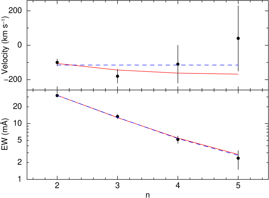
Figure 12: Equivalent width and line centroid for the 1s–2p to 1s–5p lines of O viii, plotted versus principal quantum number $n$ of the upper level. The predicted values for model 1 are shown as dashed lines, those for model 2 as solid lines.

For O viii we have measured velocities and equivalent widths for the 1s–2p to 1s–5p lines (Table 3). We have tried different models. The first model consists of a single Gaussian absorption line, with free centroid, width and column density. Model 2 has two Gaussian components, with the centroids frozen to the values given in Table 4 as derived from the O vi troughs, but with the widths and column densities free parameters. The results are shown in Table 12 and Fig. 12. Both models give a good fit and cannot be distinguished on statistical grounds. The total column densities for both models are the same within their error bars, and also the sum of the width of the Gaussians for Model 2 is consistent with the width of the single Gaussian for Model 1. Apparently, as far as the determination of total line width and column density is concerned, the detailed column density distribution as a function of velocity is not very important. This can be understood as the strongest line with the best statistics (1s–2p) has a large optical depth (12.7 and 4.9 for the two components in model 2). The line core is thus black, the line shape rather “rectangular” and to lowest order approximation the width of the line is given by the sum parts of the spectrum where the core is black.

For Model 2, the total width for each of the components agrees well with the total width of components 1–3 and 4–7 of the O vi line. Thus, O viii originates from multiple components, but the fastest outflow components have a larger column density than the slower outflow components.

Table 13: Parameters of the velocity components for O vii in the outflow of Mrk 509. Numbers in parenthesis were kept fixed.

Parameter	Model 1	Model 2
		comp. 1–3	comp. 4–7
$v$ (km s-1)	$-102\pm 17$	($-329$)	($+46$)
$\sigma$ (km s-1)	$96\pm 9$	$80(>60)$	$51\pm 8$
$N_{\rm ion}$ ($10^{20}$ m-2)	$5.9\pm 0.7$	$0.7(-0.1,+0.6)$	$6.9\pm 1.6$
		total: $7.8\pm 1.4$
$\chi^{2}$	22.57	12.93
d.o.f.	5	4

We have done a similar analysis for the 1s–2p to 1s–5p lines of O vii (Table 13). The velocity broadening is consistent with what we obtained for O viii, although there is somewhat larger uncertainty. For O vii, however, the low velocity components 4–7 have clearly the highest column density, similar to what was found for O vi (Kriss et al. 2000).

8 Statistics

Local continuum fits to RGS spectra in spectral bands that have few lines yield in general $\chi^{2}$ values that are too low. This is an artifact of the SAS procedures related to the rebinning of the data. Data have to be binned from the detector pixel grid to the fixed wavelength grid that we use in our analysis. However, the bin boundaries of both grids do not match. As a consequence of this process, the natural Poissonian fluctuations on the spectrum as a function of detector pixel are distributed over the wavelength bin coinciding most with the detector pixel and its neighbours. In addition, there is a small smoothing effect caused by pointing fluctuations of the satellite. Due to this tempering of the Poissonian fluctuations, $\chi^{2}$ values will be lower for a “perfect” spectral fit.

We have quantified the effect by fitting a linear model $F_{\lambda}=a+b\lambda$ to fluxed spectra in relatively line-poor spectral regions, in 1 Å wide bins in the 7–10, 17–18 and 35–38 Å ranges. The median reduced $\chi^{2}$ is 0.72, with a 67 % confidence range between 0.65 and 0.79. Over the full 7–38 Å range, we have at least 400 counts (and up to 3000 counts) in each bin of $\sim$0.02 Å width. Therefore, the Poissonian distribution is well approximated by the Gaussian distribution, and the usage of chi-squared statistics is well justified.

The rebinning process conserves the number of counts, hence the nominal error bars (square root of the number of counts) are properly determined. The lower reduced $\chi^{2}$ is caused by the smoothing effect on the data. For correct inferences about the spectrum, such a bias in $\chi^{2}$ is not appropriate. As we cannot change the observed flux values, we opt to multiply the nominal errors on the fluxes by $\sqrt{0.72}=0.85$, in order to get acceptable values for ideal data and models.

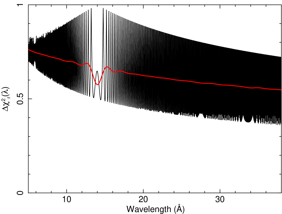
Figure 13: Relative contribution per wavelength bin to the reduced $\chi^{2}$. Calculated and shown is the ratio ${\rm Var}[Y_{i}]/{\rm E}[Y_{i}]$ (see text). The thick line is a low-resolution spline approximation showing the trends in the average value.

As a final check we have made a more robust estimate of the effect. For RGS1, the wavelength channel number $c_{\lambda}$ as a function of dispersion angle channel $c_{\beta}$ can be approximated well with

$$c_{\lambda}=5.3708506+0.66942769c_{\beta}+1.12824091\times 10^{-4}c_{\beta}^{2}.$$ (20)

Locally, if the spectrum on the $\beta$-grid is given by a set of random variables $X_{j}$ and the spectrum on the wavelength grid is given by $Y_{i}$, then we have

$$Y_{i}=\sum\limits_{j}f_{ij}X_{j},$$ (21)

for a small number of bins $j$ around the corresponding $\beta$-channel given by (20). It is here important to note that while the $X_{j}$ variables are statistically independent, the $Y_{i}$ variables are in general not statistically independent. Typically, the $f_{ij}$ factors are proportional to the overlap of wavelength bin $j$ with $\beta$-bin $i$. The clue is now that from elementary statistical considerations we have for the expected value of $Y_{i}$ and the variance

$${\rm E}[Y_{i}]=\sum\limits_{j}f_{ij}{\rm E}[X_{j}],$$ (22)

$${\rm Var}[Y_{i}]=\sum\limits_{j}f_{ij}^{2}{\rm Var}[X_{j}].$$ (23)

For instance, when the single $\beta$-bins $j$ would be exactly redistributed over two adjacent $\lambda$-bins, then there are two $f$-values, each $=0.5$, and we have ${\rm Var}[Y_{i}]/{\rm E}[Y_{i}]=0.5{\rm Var}[X_{j}]/{\rm E}[X_{j}]$, where the factor 0.5 comes from $0.5^{2}+0.5^{2}$. We have done the calculation exactly using the grids related through (20), and show our result in Fig. 13.

9 Conclusion

9.1 Wavelength scale and spectral resolution

By using five different methods, we have obtained a consistent wavelength scale with an accuracy of about 1.8 mÅ, four times better than the nominal wavelength accuracy of RGS. The only slightly deviant diagnostic remains the neutral gas in our galaxy (O i and N i), which are off from the mean by $8.8\pm 3.8$ mÅ (2.3$\sigma$). The systematics due to blending (for O i) and the lack of sufficiently reliable RGS data for N i may be slightly larger than we have estimated.

Our work shows that in cases like ours a dedicated effort to improve the wavelength scale is rewarding. As we showed, at this level of accuracy, Doppler shifts due to the orbit of Earth around the Sun become measurable. It also allows us to use X-ray lines as tools to study the dynamics of the outflow and the Galactic foreground at a level beyond the nominal resolution of the instrument (see Sect. 7).

9.2 Effective area corrections

The corrections that we have derived for the relative effective area of both RGS detectors, as well as for the relative effective area of both spectral orders are at the few percent level but should be taken into account for the high statistical quality spectrum that we consider here. This is due to the fact that there are data gaps for each individual RGS, but each time at a different wavelength range. Without such a correction, there would be artificial jumps at the boundaries of these regions of the order of a few percent. This leads any spectral fitting package to attempt to compensate for this by enhancing or decreasing astrophysical absorption lines or edges, in the hunt for the lowest $\chi^{2}$ value.

A disadvantage of our method is of course that the “true” effective area and hence absolute flux is known only to within a few percent, and the deviations are wavelength-dependent. In our subsequent spectral fitting (Detmers et al. 2011) we compensate for this by using a spline for the AGN continuum. This is clearly justified, as one might worry about the intrinsic applicability of e.g. pure power-law or blackbody components when the flux can be measured down to the percent level accuracy. The “true” continua may contain all kinds of features including e.g. relativistically broadened lines (e.g. Branduardi-Raymont et al. 2001; Sako et al. 2003) that can be discerned only in the highest-accuracy data, such as the present one.

9.3 Combination of spectra

The reduction of the combined response matrices of our 40 spectra with 2 Gb of memory into a single spectrum and response file of only 8 Mb, a reduction by more than two orders of magnitude, allows us to make complex spectral fits. In the most sophisticated models used by Detmers et al. (2011) the number of free parameters approaches 100, and without this efficient response matrix the analysis would have been impossible.

9.4 Final remarks

Due to the high statistical quality of our data, the binning problems mentioned in Sect. 8 became apparent. In many RGS spectra that have been obtained during the lifetime of XMM-Newton, the statistical quality of the spectra is not good enough to detect this effect. Still, this could imply that when users obtain a fit with reduced chi-squared of order unity, the fit is formally not acceptable because an ideal fit would yield a smaller reduced chi-squared. Clearly, here more work needs to be done to alleviate the problem, but due to the discretisation of wavelength in the detector corresponding to the natural size of the CCD pixels there is some natural limitation to what can be done. Even in the best observations there is always some small scatter in the satellite pointing, making some rebinning necessary.

Overall, however, the calibration of RGS is at a fairly advanced stage. Only for exceptionally good spectra like the Mrk 509 spectrum that we discussed here the sophisticated tools developed in this paper are needed, although also for weaker sources our improvements can be beneficial for the analysis. Our tools are publicly available as auxiliary programs (rgsfluxcombine, rgs_fmat) in the SPEX distribution.