VLBI-selected sample of Compact Symmetric Object candidates and frequency-dependent position of hotspots

Abstract

Context. The Compact Symmetric Objects (CSOs) are small ($<1$ kiloparsec) and powerful extragalactic radio sources showing emission on both sides of an active galactic nucleus and no signs of strong relativistic beaming. They may be young radio sources, progenitors of large FR II radio galaxies.

Aims. We aim to study the statistical properties of CSOs by constructing and investigating a new large sample of CSO candidates on the basis of dual-frequency, parsec-scale morphology.

Methods. For the candidate selection we utilized VLBI data for 4170 extragalactic objects obtained simultaneously at 2.3 and 8.6 GHz ($S$ and $X$ band) within the VLBA Calibrator Survey 1-6 and the Research and Development – VLBA projects. Properties of their broad-band radio spectra were characterized by using RATAN-600 observations. Numerical modeling was applied in an attempt to explain the observed effects.

Results. A sample of 64 candidate CSOs is identified. The median two-point $S$–$X$ band spectral index of parsec-scale hotspots is found to be $-0.52$; with the median brightness temperature $\sim 10^{9}$ K at $X$ band. Statistical analysis reveals a systematic difference between positions of brightest CSO components (associated with hotspots) measured in the $S$ and $X$ bands. The distance between these components is found to be on average $0.32\pm 0.06$ mas greater at $8.6$ GHz than at $2.3$ GHz.

Conclusions. This difference in distances cannot be explained by different resolutions at the $S$ and $X$ bands. It is a manifestation of spectral index gradients across CSO components, which may potentially provide important physical information about them. Despite our detailed numerical modeling of a CSO hotspot, the model was not able to reproduce the magnitude of the observed positional difference. A more detailed modeling may shed light on the origin of the effect. Multifrequency follow-up VLBI observations of the selected sample are needed to confirm and study newly identified CSOs from the list presented here.

1 Introduction

Compact Symmetric Objects (CSOs) are small ($<1$ kiloparsec), powerful extragalactic radio sources that show emission on both sides of an active galactic nucleus (Wilkinson et al., 1994; Readhead et al., 1996). In contrast to the majority of compact radio sources, relativistic beaming effects are believed to be small in CSOs owing to their orientation close to the plane of the sky. The parsec-scale core that marks position of the central engine is often weak or not detected at all. Kinematic studies of CSOs reveal no superluminal motion and suggest source ages of a few hundred to a few thousand years (Owsianik & Conway, 1998; Polatidis, 2009). CSOs may be progenitors of large-scale Fanaroff-Riley type II radio galaxies (Fanti et al., 1995; Readhead et al., 1996; Perucho & Martí, 2002). To draw solid conclusions about the properties of CSOs as a class, it is important to construct a large representative sample of them.

An interesting side effect of an investigation of a large CSO candidate sample is the possibility of finding a supermassive binary black hole pair (Maness et al., 2004; Rodriguez et al., 2006; Tremblay et al., 2009) that can mimic a CSO. Such an object would have two compact radio components that share the typical characteristics of the core: flat spectrum, high brightness temperature $T_{\mathrm{b}}$, and complex flux variability pattern. It has also been suggested that true CSOs are the likely hosts of supermassive black hole binaries (Willett et al., 2010). Finally, CSOs may be useful as calibrators for continuum observations of other radio sources thanks to their stable flux density and low fractional polarization (Taylor & Peck, 2003).

The largest homogeneously selected CSO sample to date is the COINS sample by Peck & Taylor (2000). An initial list of candidates for this sample was selected from Pearson & Readhead (1988) and Caltech–Jodrell Bank (Taylor et al., 1994) VLBI surveys and from the first VLBA Calibrator Survey (Beasley et al., 2002). Dedicated multifrequency polarimetric VLBA observations of the candidates have been performed to distinguish between true CSOs and contaminating core-jet type sources. The sample was further extended to the northern and southern extremities of the VLBA Calibrator Survey by Taylor & Peck (2003). Another CSO sample based on the VLBA Imaging and Polarization Survey is being constructed by Tremblay et al. (2009).

In this paper we present a list of CSO candidates selected by using publicly available $S$ band (central frequency 2.3 GHz) and $X$ band (central frequency 8.6 GHz) VLBI data collected in the course of the VLBA Calibrator Surveys (VCS) 1 to 6 by Beasley et al. (2002), Fomalont et al. (2003), Petrov et al. (2005, 2006), Kovalev et al. (2007), Petrov et al. (2008), and the Research and Development VLBA program (RDV, e.g., Fey et al., 1996; Fey & Charlot, 1997; Pushkarev & Kovalev, 2008; Petrov et al., 2009). We discuss the basic properties of the compiled sample of CSO candidates including an unexpected systematic difference in CSO component positions measured at the lower and higher frequencies and our attempt to reproduce this effect with detailed numerical modeling.

2 The VLBI-selected sample of CSO candidates and its basic characteristics

Among 4170 radio sources observed in the course of VCS and RDV VLBI experiments, we selected a list of 64 CSO candidates that meet the following criteria.

1. S and X band images show two dominating components of comparable brightness that are presumed to be hotspots on both sides of a two-sided jet.

2. Each component is detected in the $S$ and $X$ bands with signal-to-noise ratios greater than five.

3. Most of the residual emission, if present, is located between the two brightest components. This emission may come from the core, mini-lobes, or the jet itself.

The third criterion is meant to distinguish CSO from sources with a bright core and one-sided jet showing a single jet component comparable in brightness to the core.

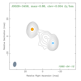
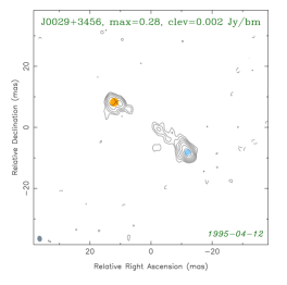
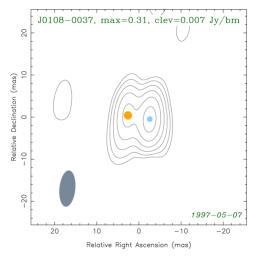
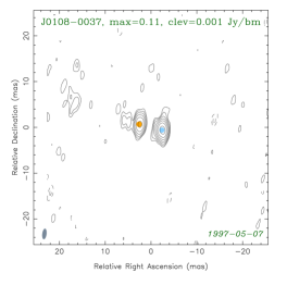
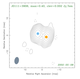
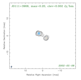
Figure 1: Dual-frequency simultaneous 2 and 8 GHz CLEAN images. The lowest contour value ‘clev’ is chosen at four times the rms level, and the peak brightness is given by ‘max’ (Jy/beam). The contour levels increase by factors of two. The dashed contours indicate negative flux. The beam is shown in the bottom left corner of the images at the half-power level. An epoch of observation is shown in the bottom right corner. Blue and orange spots indicate Gaussian model components 1 and 2, respectively. The brightness distribution is shown at the full resolution of naturally weighted data, while the model components are fitted in a restricted $uv$-range that is common to both bands, see § 4 for details.

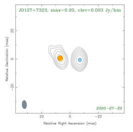
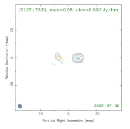
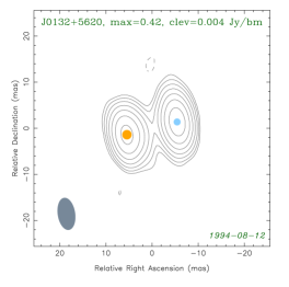
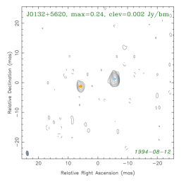
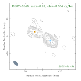
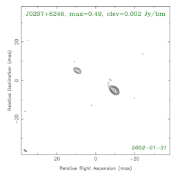
Figure 1: continued

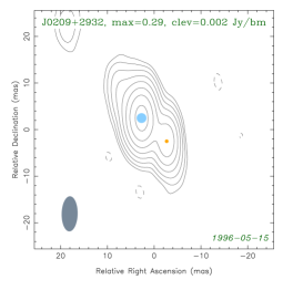
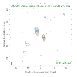
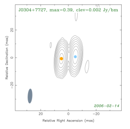
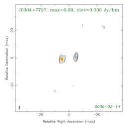
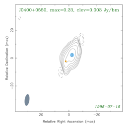
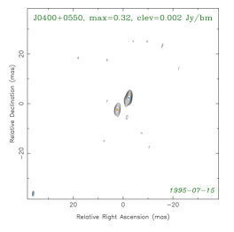
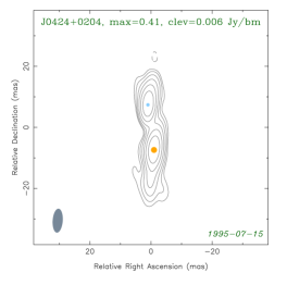
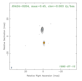
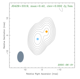
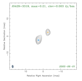
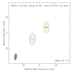
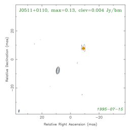
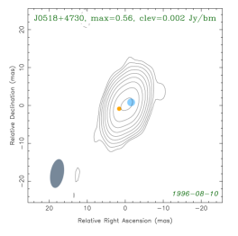
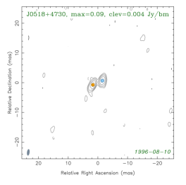
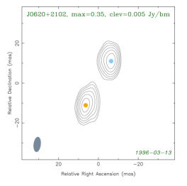
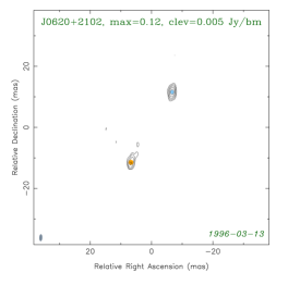
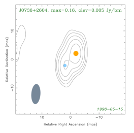
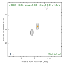
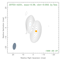
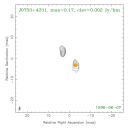
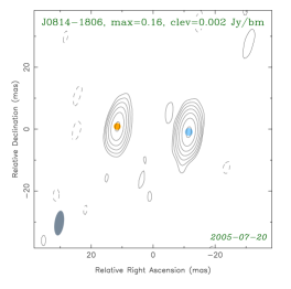
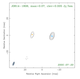
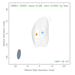
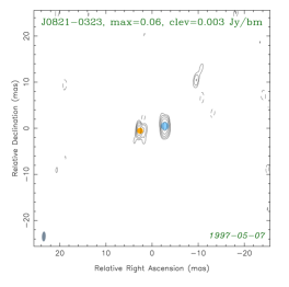
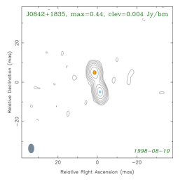
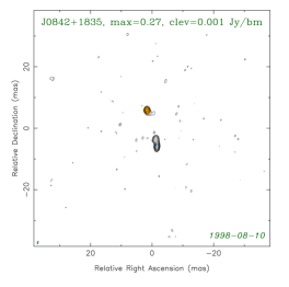
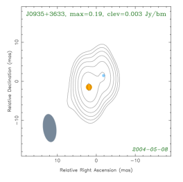
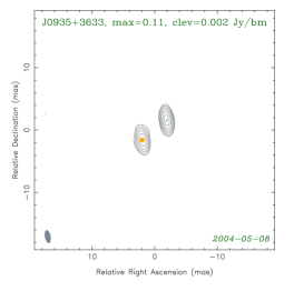
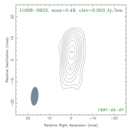
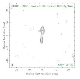
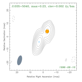
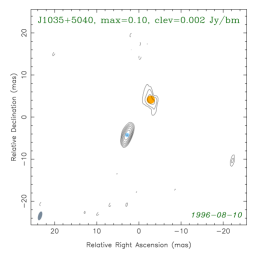
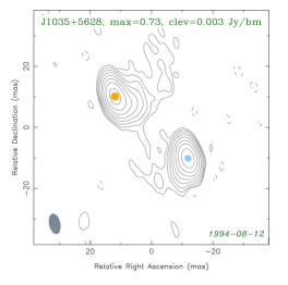
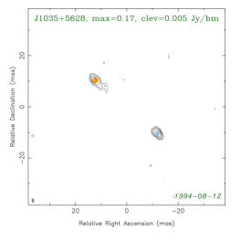
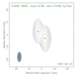
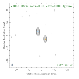
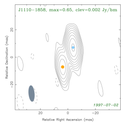
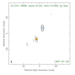
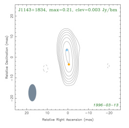
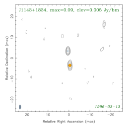
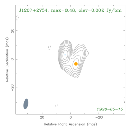
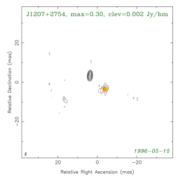
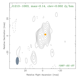
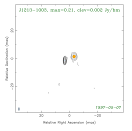
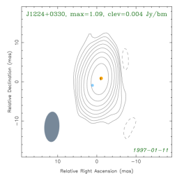
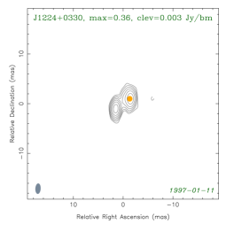
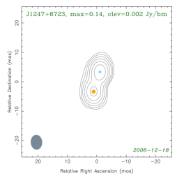
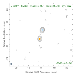
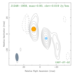
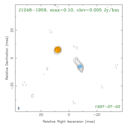
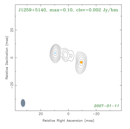
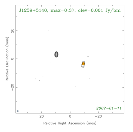
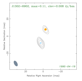
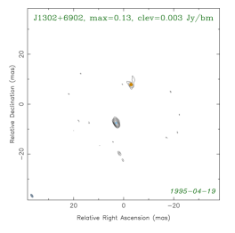
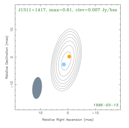
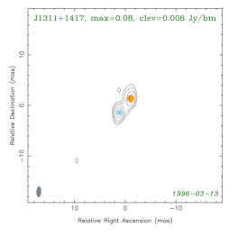
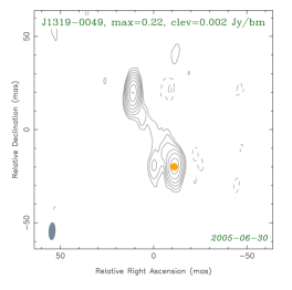
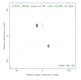
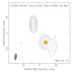
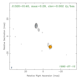
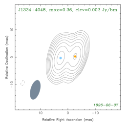
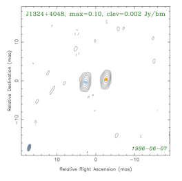
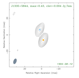
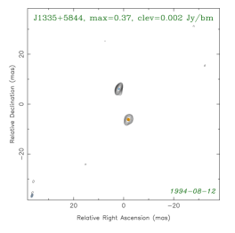
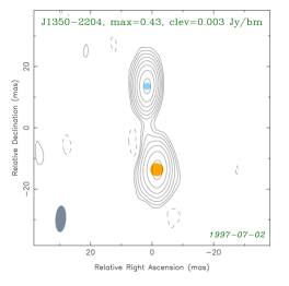
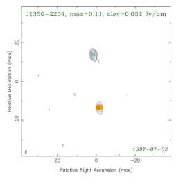
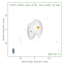
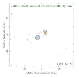
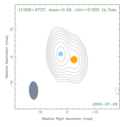
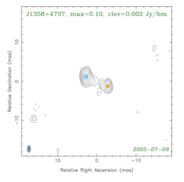
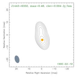
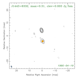
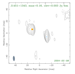
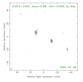
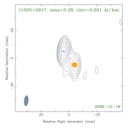
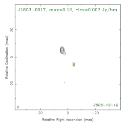
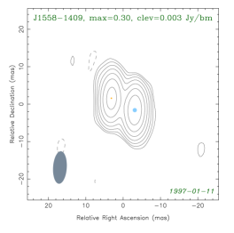
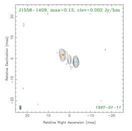
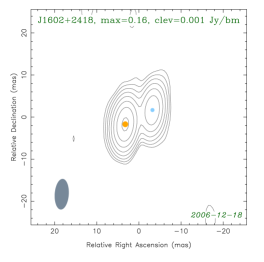
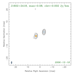
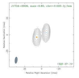
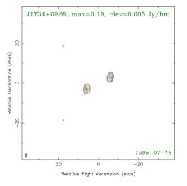
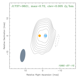
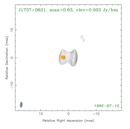
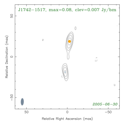
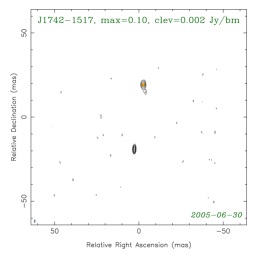
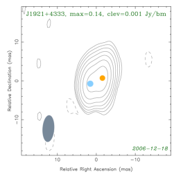
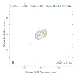
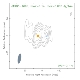
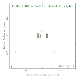
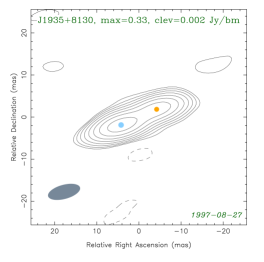
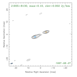
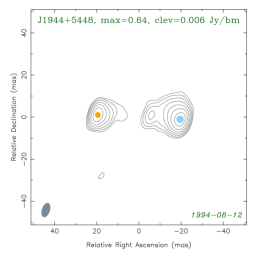
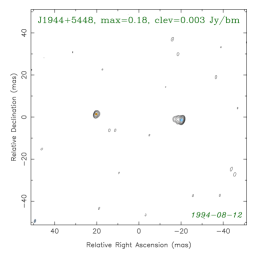
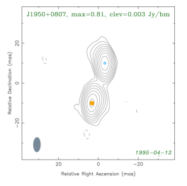
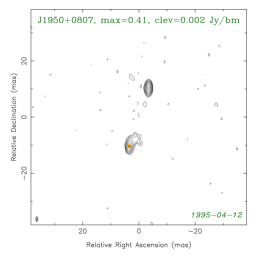
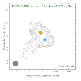
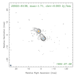
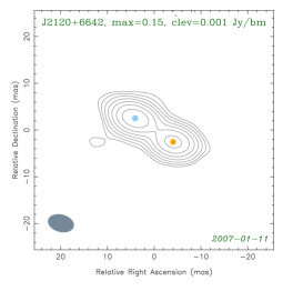
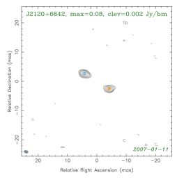
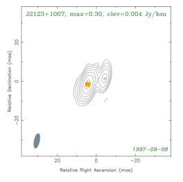
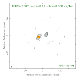
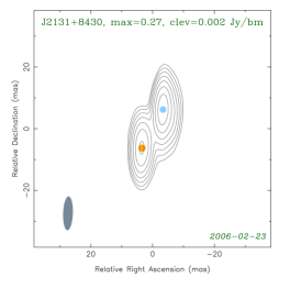
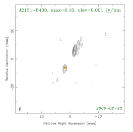
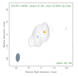
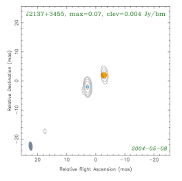
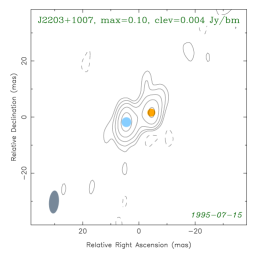
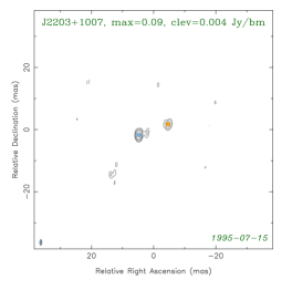
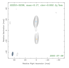
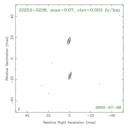
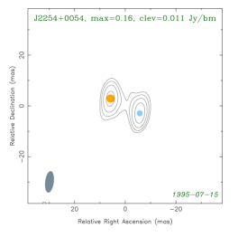
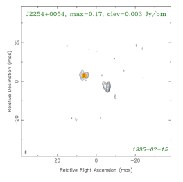
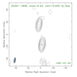
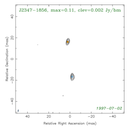
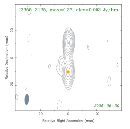
Figure 1: continued

The list of selected sources is presented in Table LABEL:table:srclist. We followed Fomalont (1999) to estimate errors of the model component parameters. The dual-frequency $S$- and $X$-band, naturally weighted CLEAN images of the sources are shown in Fig. 1. The lowest contour level was chosen at four times the image rms, and plotted contour levels increased by a factors of two. The beam is shown in the bottom left-hand corner of each image. Blue and orange spots indicate Gaussian model components 1 and 2 from Table LABEL:table:srclist, respectively. Table LABEL:table:srclist and Fig. 1 are available in the electronic version of the paper.

The information about broad-band radio spectra of the sources was obtained from the RATAN-600 multifrequency multi-epoch $1$–$22$ GHz observations in 1997-2006 (Kovalev et al., 1999; Kovalev et al., 2002) and data from the literature collected by means of the CATS database (Verkhodanov et al., 2005). Among the selected CSO candidates we identified 30 GHz–Peaked Spectrum (GPS) sources, 12 steep spectrum sources, and 22 flat spectrum sources. For a discussion of GPS sources observed by the RATAN-600, see Sokolovsky et al. (2009) and Sokolovsky & Kovalev (2008). We consider sources with peaked or steep spectra as the most promising CSO candidates.

Among 64 selected candidates, 13 are part of the COINS CSO sample (Peck & Taylor, 2000) and three more sources are listed as rejected candidates for the COINS sample on the basis of their parsec-scale spectra and polarization properties. Two of them (0357$+$057, 1734$+$063) have flat single-dish spectra, while the third source (0839$+$187, also known as OJ 164) shows a spectral peak at $\sim 1.2$ GHz. The last source is an important example of a kind of GPS quasar with core-jet morphology, which may contaminate CSO samples, including the one presented in this paper.

Optical identifications and redshifts of 28 CSO candidates are available from the Véron-Cetty & Véron (2006) catalog, while 36 objects have no known optical counterpart. Among the identified sources, 19 are quasars, seven are active galaxies, and two are BL Lac type objects. The boundary between quasars and active galaxies (which include Seyferts and Liners) is somewhat arbitrarily chosen in the Véron-Cetty & Véron (2006) catalog at an absolute optical magnitude $M_{B}=-23$. Since quasars are intrinsically brighter in the optical band, they are more likely to be detected than are radio galaxies. A similar effect for GPS sources was reported by Sokolovsky et al. (2009). However, we expect that at least half of the CSO candidates presented in this paper are associated with quasars. It is remarkable that the compact double radio structure that we associate with candidate CSOs is found in objects characterized by a wide range of optical luminosities (quasars, radio galaxies) and a variety of radio spectrum shapes (steep, GPS, flat).

None of the selected radio sources has a $\gamma$-ray counterpart in the Fermi Large Area Telescope first-year catalog (1FGL; Abdo et al. 2010a), the largest catalog of GeV sources to date. Since the extragalactic $\gamma$-ray sky is dominated by blazars (e.g., Abdo et al., 2010b; Kovalev, 2009; Thompson et al., 1993), this provides additional reassurance that the selected sample is not strongly contaminated by relativistically beamed objects.

3 Properties of the dominating parsec-scale components

As described above, we have selected sources that only show two dominant components both in the $S$ and $X$ bands. We associate these components with hotspots at opposite ends of a two-sided jet. To quantify the position, flux density, and size of the hotspots, each source was modeled in the visibility ($uv$) plane by two circular Gaussian components using the Difmap software (Shepherd, Pearson, & Taylor, 1994). To minimize the effect of the resolution difference between bands, only $uv$-range covered by both $S$- and $X$-band data was used for the modeling.

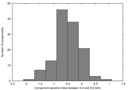
Figure 2: $S$–$X$ band spectral index, $\alpha$, distribution for bright CSO components ($S\propto\nu^{\alpha}$).

The distribution of the two-point, simultaneous $S$–$X$ band spectral index of the components is presented in Fig. 2. It shows values in the range from $-1.83$ to $+0.99$ with the median of $-0.52$. It is evident that the majority of the observed components in the selected CSO candidates have spectral indices that are not typical of flat-spectrum cores.

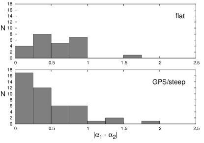
Figure 3: Absolute difference between $S$–$X$ band spectral indices of the components 1 ($\alpha_{1}$) and 2 ($\alpha_{2}$) for objects of various spectral types as presented in Table LABEL:table:srclist. The Kolmogorov-Smirnov test indicates at the 94 % confidence level that the distributions are different.

The similarity of broad-band spectra of the two dominant parsec-scale features is expected to indicate a true CSO. To establish this similarity, multifrequency VLBI follow-up observations of the selected sample of still unconfirmed CSO, similar to the study by Peck & Taylor (2000), are needed. Comparing the two-point simultaneous $S$–$X$ band spectral indices available from our modeling is not sufficient. However, it may provide a hint that a source is probably a true CSO, since a majority of true CSOs (e.g., from the COINS sample) are found to have similar $S$–$X$ band spectral indices, $\alpha_{1}$ and $\alpha_{2}$, for the two brightest parsec-scale components (Table LABEL:table:srclist). On the other hand, a typical core-jet source is expected to show significantly different spectral indices of the two dominant components (absolute difference near to or greater than 0.5) due to the flat radio spectrum of the synchrotron self-absorbed core and steep-spectrum synchrotron radiation of the optically thin jet feature. Figure 3 presents the distribution of the absolute difference $|\alpha_{1}-\alpha_{2}|$ of the indices for sources in our sample separated on the basis of their single-dish radio spectrum type — GPS/steep versus flat. Figure 3 supports the assumption that GPS/steep spectrum sources tend to have similar spectra of the two brightest parse-scale components, while flat spectrum sources tend to have dominant parsec-scale components with different spectra. The median component spectral index differences are $0.58$ for the flat and $0.34$ for the GPS/steep subsample. The Kolmogorov-Smirnov test indicates at the 94 % confidence level that the distributions may be different. Most of the contaminating core-jet sources — not true CSO — are expected to be found within the flat-spectrum subsample of the CSO candidates list.

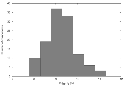
Figure 4: Brightness temperature distribution (measured at $X$ band) for bright CSO components.

We have also estimated the brightness temperature of the components at $X$ band, which is found to be typically $T_{\mathrm{b}}\sim 10^{9}$ K in the observer’s frame (see Table LABEL:table:srclist and Fig. 4) — systematically lower than the one measured in the parsec-scale cores of typical bright extragalactic Doppler-boosted core-jet sources (e.g., Kovalev et al., 2005; Pushkarev & Kovalev, 2011). The values of $T_{\mathrm{b}}$ presented in Table LABEL:table:srclist are computed using component parameters derived from modeling restricted $uv$-range data for consistency with parameters presented in other columns of Table LABEL:table:srclist. Brightness temperatures derived from the modeling, which takes full $uv$-range available at $X$ band into account, are consistent within a factor of two with the values obtained from the restricted $uv$-range models.

4 Frequency-dependent component position

5

(a) $2.3$ GHz

(b) $8.6$ GHz

Figure 5: $uv$-coverage obtained for the CSO candidate source J1357$+$4353 at $2.3$ GHz (5a) and $8.6$ GHz (5b) observed on 2002 May 14 within the VCS2 (Fomalont et al., 2003) VLBA experiment.

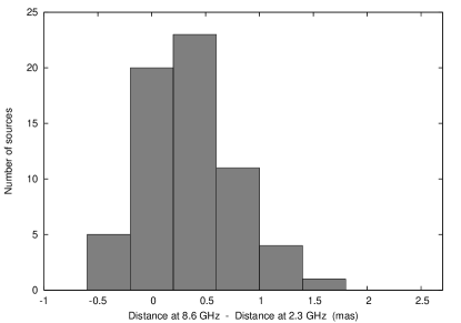
Figure 6: Difference in distances between two dominant source components measured in $X$- (8.6 GHz) and $S$ (2.3 GHz) bands. The median value of the distribution is $0.27$, which is significantly ($>99.9$ % probability according to the sign test) greater than zero.

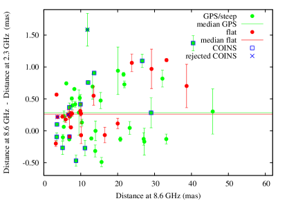
Figure 7: Difference in distances between two dominant source components measured in the $S$ and $X$ bands as a function of distance measured in the $X$ band. Green points represent GPS and steep spectrum sources, red points represent flat spectrum sources. Objects included in the COINS sample are marked with blue squares, while objects rejected from the COINS sample as probable core-jet sources are marked with blue crosses. The green line denotes the median distance difference for GPS/steep spectrum sources, the red line marks the same for flat spectrum sources.

Interestingly, we have found that distances between the two dominant parsec-scale components are systematically greater when measured in the $X$ band (8.6 GHz) than those measured in the $S$ band (2.3 GHz). An indication was first based on the full $uv$-range modeling at each frequency. The mean difference in CSO component separation measured in the $S$ and $X$ bands was found to be $0.40\pm 0.07$ mas (median value $0.34$ mas).

The distance between the two outer components of a CSO may appear different if measured at different frequencies because of (i) an observational effect caused by difference in $uv$-coverage, hence the resolution in $S$ and $X$ bands or (ii) real spectral index gradients across the components. The second possibility may potentially provide important information about physical conditions around the termination shock of a CSO jet, particle acceleration efficiency, and cooling rate, as investigated in Sect. 5. To eliminate the former possibility, we redid the model fitting and component position analysis restricting the used $uv$-range to spatial frequencies common to $S$- and $X$-band data. The mean difference was found for the restricted case to be $0.32\pm 0.06$ mas, while the median value is $0.27$ mas if all 64 CSO candidates are considered. These values are consistent with those obtained using the full $uv$-range on the one–$\sigma$ level, indicating that the difference in $uv$-coverage between the $S$ and $X$ bands only has a minor effect on the derived component positions. The magnitude of the difference between the values obtained for the full and restricted $uv$-range is comparable to the values obtained in our numerical modeling (Section 5, Table 2) where the effect of resolution difference was simulated in the image plane by convolving the high-resolution model jet image with Gaussian beams of different sizes.

In the following discussion and analysis we use the results obtained using the $uv$-range restricted to the spatial frequencies common to both bands in order to completely eliminate the systematic effect associated with the difference in resolution. A typical $uv$-coverage for the archival $S$- and $X$-band VLBI data used to select CSO candidates is presented in Fig. 5 (available in the online version of the paper). Figure 6 presents the distribution of the distance differences. We did not recalculate this value in the source frame because many sources in our sample have no redshift information available. The sign test (e.g., Mendenhall et al., 1989) confirms that the observed median difference is indeed greater than zero with a probability higher than 99.99 %. The sign test was chosen because it is a non-parametric test and makes very few assumptions about the nature of the distribution under investigation. Figure 7 illustrates the position difference as a function of component distance measured in the $X$ band for flat- and GPS/steep-spectrum CSO candidates. The correlation analysis indicates a positive correlation between the $S$–$X$ band distance difference and the distance measured at $X$ band with the Pearson’s correlation coefficient $r=0.35$, which corresponds to a 99.4 % probability of true correlation at the given sample size, if all candidates are considered together.

The observed frequency-dependent difference in component positions could be trivially explained as the well known “core shift” effect (e.g., Lobanov, 1998; Kovalev et al., 2008; Sokolovsky et al., 2011) if the presented sample of CSO candidates is heavily contaminated with core-jet type sources where one of the two observed bright components is actually a core instead of a hot spot. Spectral index of a component should be flat or inverted ($\alpha\geq 0$) if it is the core, so one may expect a positive correlation between $\alpha$ and the distance difference. However, no such correlation is observed. Also, no correlation was found between $T_{\mathrm{b}}$ of the first component and the observed distance difference (Table LABEL:table:srclist). Moreover, as shown in §3, most of the dominating parsec-scale features have steep spectral indices and relatively low brightness temperatures, which is not typical of Doppler-boosted, opaque parsec-scale cores.

To further test the core shift possibility, we divided the CSO candidates into two groups based on their single-dish radio spectra similar to the analysis presented in Fig. 3. The first group contained flat-spectrum sources that are more likely to be blazars with core-jet type morphology. The second group included sources with peaked and steep spectra, which are more likely to be true CSO. For the flat-spectrum group, the mean position difference was found to be $0.33\pm 0.08$, median value $0.26$, with $>99.9$ % probability that the median value is greater than zero. For the GPS/steep spectrum group, the mean difference is $0.31\pm 0.08$, the median value $0.28$, with $>99.9$ % probability of it being higher than zero. A Kolmogorov-Smirnov test can exclude ($p=0.06$) the possibility that the frequency-dependent position differences observed in flat-spectrum and GPS/steep-spectrum sources are drawn from the same parent distribution.

It is widely accepted (e.g., Stanghellini et al., 1997; Ostorero et al., 2010) that CSOs are often found among GPS sources identified with galaxies (as opposed to blazars). In the presented sample of CSO candidates there are only five GPS sources associated with galaxies, which is not enough for a statistical analysis. However, we note that among these five sources (which should be considered the best CSO candidates), four show a positive difference between component distances measured at $8.6$ and $2.3$ GHz.

Overall, it seems highly unlikely that the systematic difference in component positions at $2.3$ and $8.6$ GHz in the selected sources can be attributed to the core shift effect in core-jet type sources contaminating the CSO candidate sample. Intrigued by the observed effect, we have turned to detailed numerical modeling in search of an explanation.

5 Discussion

When the jet flow crosses the hotspot, it is deflected and starts to flow backwards towards the nucleus. This is known as the backflow. When radio-emitting particles cool in such a backflow, we expect the higher energy emission (caused by the faster cooling high-energy particles) to be concentrated closer to the hotspot, whereas the lower energy emission (from the slower cooling low energy particles) should be seen farther away towards the nucleus, while these particles are being dragged by the backflow. Thus, this should generate a spatial separation between the peaks of the emission at higher and lower frequencies such that the high-frequency peak is observed farther away from the nucleus than the lower frequency one. This is a possible cause of the observed bias.

We attempted to test this hypothesis by computing radio emission from simulated relativistic jets. The code and initial setup is similar to that of Perucho & Martí (2007). We performed two simulations, one with a one-sided jet (M1) and a second one with a two-sided jet (M2), by changing the boundary conditions at the inlet. The radio emission is computed using the SPEV code (Mimica et al., 2009).

The simulated jets are injected with an initial velocity $0.95$ c and the Mach number $1.66$. The density contrast between the jets and external medium at the injection point ($10$ pc from the nucleus) is $10^{-5}$, and their initial radius is $2$ pc. The jet composition is purely leptonic and the external medium is composed of the neutral hydrogen. We assume the profile of the external medium in a typical radio galaxy like 3C 31 (Perucho & Martí, 2007; Hardcastle et al., 2002).

The jets were evolved until they reach the distance of $110$ pc from the nucleus. We used these as an input for the SPEV code, and produced synthetic radio images at $2.3$ and $8.6$ GHz, assuming the jet angle to the line of sight to be $70^{\circ}$. Since the simulations do not include magnetic fields, for the purpose of computing the emission, we assumed a randomly oriented magnetic field in a fraction of equipartition with the thermal fluid, whereby the ratio of magnetic to internal energy density was fixed to $\epsilon_{B}=10^{-3}$. The relative properties of the emission at $2.3$ and $8.6$ GHz are expected to depend only weakly on the value of $\epsilon_{B}$ because the radio frequencies are always below the cooling frequency for the particle distribution. The typical value of the magnetic field at the injection point is $\approx 20\mu$G.

SPEV code uses Lagrangian particles as markers of the nonthermal particles responsible for the radio emission (details can be found in Mimica et al. 2009). In the current work we assume that these Lagrangian particles are inserted into the jet at the injection point and their spatial, temporal and spectral evolution is followed by taking synchrotron and adiabatic losses into account. We also have the possibility of accelerating additional particles in strong shock waves (e.g., Mach disk). We denote such models with a suffix ”s” (M1s and M2s). For both types of particle injection (at the jet injection point or in the shocks), we assume that the total particle number density is proportional to the thermal fluid density and that the total particle energy density is proportional to the fluid internal energy density. We fix the power-law index of the nonthermal energy distribution at the time of injection to $2.25$. These assumptions allow us to determine the lower cutoff of the particle injection spectrum (see Mimica et al. 2009 for more details). To determine the upper cutoff we equate the synchrotron cooling time with the electron acceleration time (see Mimica et al. 2010 for a more detailed discussion of the upper cutoff).

The synthetic radio maps obtained from the simulations have much better resolution than typical VLBI observations. In order to be able to compare them directly we artificially degrade the quality of synthetic radio maps to that of the observations. To this end we compute degraded images assuming the source to be at two redshifts, $z=0.04$ and $z=1$. We note that the angular resolution of the original synthetic radio maps is $0.14$ and $0.014$ milliarcseconds at $z=0.04$ and $z=1$, respectively. We convolve the images with a Gaussian beam whose characteristic half-power size is $6$ and $1.8$ milliarcesonds at $2.3$ and $8.6$ GHz, respectively. In Fig. 8 we show radio maps for model M1.

Table 2: Difference in positions of the peaks at $8.6$ and $2.3$ GHz.

Model	$\Delta_{0.04}$	$\Delta_{1}$
index	(mas)	(mas)
M1s	$<0.14$	$0.11$
M1	$<0.14$	$0.11$
M2s	$<0.14$	$0.11$
M2	$<0.14$	$0.11$
M2cs	$-0.28$	$0.055$
M2c	$-0.28$	$0.055$

Note: $\Delta_{0.04}$ and $\Delta_{1}$ are the differences for the source redshift of $0.04$ and $1$, respectively. Positive values indicate that the peak at the $8.6$ GHz is farther away from the nucleus than at $2.3$ GHz. M1s and M1 stand for the one-sided jet model with and without shock acceleration, respectively. Similarly, M2s and M2 stand for the jet of the double-sided jet model, while M2cs and M2c stand for the counter jet in that same model. When the difference is smaller than the angular resolution of the unconvolved maps, we give only upper bounds.

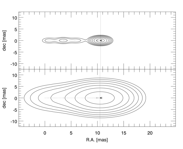
Figure 8: Synthetic radio maps at $2.3$ GHz (lower panel) and $8.6$ GHz (upper panel) of the simulated jet model M2s (see Fig. 2 in Perucho & Martí 2007 for the typical hydrodynamic structure of such simulated jets). Shades of gray show the normalized intensity of the unconvolved radio maps. Assuming that the source is located at $z=1$ contours show the degraded (convolved) image. Contour levels are 1, 2, 4, 8, 16, 32, and 64 % of the peak intensity. The bright feature in the center of each panel is the hot spot, and vertical lines denote the longitudinal position of the peak intensity in the convolved image. The difference in position of the peak at two frequencies is very small.

In Table 2 we summarize the results of our simulations. We see that the results do not confirm the hypothesis. Although models M1, M1s, M2, and M2s, as well as models M2c and M2cs for $z=1$, show the expected trend, the differences are too small to be detected, which can also be seen in Fig. 8, where vertical lines denote the position of the intensity peak. No such trend is observed for models M2c and M2cs for $z=0.04$.

The population of the nonthermal particles is dominated by the synchrotron cooling close to the injection site and by the adiabatic cooling further downstream (see e.g., Mimica et al. 2009). In the synchrotron-cooling region we expect that the higher energy particles lose their energy faster than the lower energy ones, whereas in the adiabatic-cooling region they all lose the energy at the same rate. Nonthermal particles inserted at the jet injection point reach the adiabatic-cooling region long before they reach the hotspot. Although there is substantial compression of the flow in the shock, if shock acceleration is not included, this compression alone is not enough to produce another synchrotron-cooling region. Therefore, the cooling rate of the high and low energy particles is the same, and no spatial separation between high and low frequency emission is expected. If we include shock acceleration, there is a synchrotron cooling zone behind the shock, but it is not large enough to reach into the backflow, because the shock does not accelerate particles to high enough energy to produce a larger synchrotron cooling dominated zone. Therefore, the result is qualitatively the same as when shock acceleration is not taken into account. This can be seen in the unconvolved radio maps (Fig. 8), where no noticeable difference between the positions of the peaks can be observed.

The systematic difference in hotspot positions obtained in our model (Table 2) results fro the fact that the convolution beam at $2.3$ GHz is larger than at $8.6$ GHz. The former includes more emission from jet and backflow regions closer to the nucleus (blending), and this generates a shift in the position of the apparent peak towards the nucleus. This results in the aforementioned apparent position difference in our models, which is an effect of model image convolution necessary to make it comparable to real observations. The same effect should be present in observations of real sources. However, the predicted magnitude of this blending effect is still smaller than the observed position difference. This is in accordance with minor difference between the modeling results obtained using full (different resolution) and restricted (matched resolution) $uv$-range as discussed in Section 4.

In future work we intend to study two possibilities that could explain the observations. On the one hand, a much more efficient shock acceleration could produce enough high-energy particles to create a longer synchrotron cooling zone. On the other hand, the process of shear layer acceleration (e.g., Stawarz & Ostrowski 2002; Aloy & Mimica 2008) could produce continuous injection of nonthermal particles into the backflow. Small velocity gradients present there would probably result in low acceleration efficiency, lower emission frequency, and ultimately, a shift in the position of the peak of emission towards the nucleus for those frequencies.

6 Summary

We selected a sample of 64 candidate compact symmetric objects (CSOs) using simultaneous $S$ (2.3 GHz) and $X$ (8.6 GHz) band VLBI data for $4170$ compact extragalactic radio sources from the VLBA Calibrator Survey 1–6 and Research and Development VLBA projects. Broad-band radio spectra of the selected sources were characterized using multifrequency observations with RATAN–600 and archival data from the literature. Among the selected CSO candidates, we identified 30 GPS, 12 steep-spectrum, and 22 flat-spectrum radio sources. The median two-point $S$–$X$ band spectral index for dominating parsec-scale components was found to be $-0.52$, while median brightness temperature is on the order of $10^{9}$ K. A multifrequency follow-up VLBI study of the whole selected sample is needed to confirm true CSO cases.

A systematic difference in distance measured at $2.3$ and $8.6$ GHz between the outer CSO components (presumed to be associated with hotspots) was detected. The $8.6$ GHz distance was found to be larger for most sources.

The analysis excluded the blending effect as the dominant cause for the observed component position difference. Even if some CSO candidates in our sample were misclassified and have a core-jet parsec-scale morphology, our analysis rules out the apparent frequency-dependent shift in the core position (the “core shift”) as an explanation for the observed effect.

Numerical modeling of a CSO hotspot was conducted but failed to reproduce the magnitude of the observed difference. The model suggested the observational blending effect as the dominating mechanism responsible for the position difference, which is too small to solely account for the observed difference. A more detailed modeling that fully accounts for the synchrotron opacity effects and dedicated simultaneous multifrequency VLBI observations are needed to determine the exact origin of the hotspot position difference effect.

1

Table 3: List of CSO candidates selected from VCS and RDV surveys

Name	Comp.	FS (Jy)	FX (Jy)	$\alpha$	RX${}^{\text{,}}$ (mas)	T${}_{\mathrm{b}\leavevmode\nobreak\ X}$${}^{\text{,}}$ (K)	DX (mas)	$D_{X}-D_{S}$ (mas)	opt.	$z$	Comments
J0029+3456	1	1.168$\pm$0.042	0.612$\pm$0.059	$-0.50\pm 0.08$	2.00$\pm$0.18	$3\times 10^{9}$	29.06$\pm$0.23	$+0.28\pm 0.23$	a	0.517	COINS, GPS $\nu_{m}$=1.41
	2	0.835$\pm$0.021	0.227$\pm$0.035	$-1.00\pm 0.12$	2.82$\pm$0.42	$5\times 10^{8}$
J0108-0037	1	0.332$\pm$0.007	0.217$\pm$0.004	$-0.33\pm 0.02$	1.13$\pm$0.02	$3\times 10^{9}$	5.15$\pm$0.02	$-0.10\pm 0.05$	q	1.378	STEEP
	2	0.159$\pm$0.009	0.097$\pm$0.003	$-0.38\pm 0.05$	1.24$\pm$0.04	$1\times 10^{9}$
J0111+3906	1	0.496$\pm$0.005	0.540$\pm$0.081	$+0.06\pm 0.11$	1.45$\pm$0.20	$4\times 10^{9}$	5.08$\pm$0.10	$-0.27\pm 0.10$	.	…..	COINS, GPS $\nu_{m}$=4.64
	2	0.400$\pm$0.005	0.254$\pm$0.009	$-0.34\pm 0.03$	0.24$\pm$0.01	$7\times 10^{10}$
J0127+7323	1	0.267$\pm$0.006	0.096$\pm$0.005	$-0.78\pm 0.04$	1.50$\pm$0.06	$7\times 10^{8}$	13.99$\pm$0.07	$-0.00\pm 0.15$	.	…..	GPS,
	2	0.107$\pm$0.008	0.014$\pm$0.002	$-1.57\pm 0.14$	1.11$\pm$0.14	$>2\times 10^{8}$
J0132+5620	1	0.458$\pm$0.007	0.313$\pm$0.004	$-0.29\pm 0.01$	0.87$\pm$0.01	$7\times 10^{9}$	11.98$\pm$0.01	$+0.76\pm 0.03$	.	…..	COINS, GPS $\nu_{m}$=3.01
	2	0.382$\pm$0.011	0.042$\pm$0.001	$-1.70\pm 0.03$	1.06$\pm$0.03	$7\times 10^{8}$
J0207+6246	1	1.085$\pm$0.014	0.650$\pm$0.001	$-0.39\pm 0.01$	0.80$\pm$0.00	$2\times 10^{10}$	21.58$\pm$0.00	$+0.88\pm 0.03$	.	…..	GPS $\nu_{m}$=2.50
	2	0.309$\pm$0.014	0.056$\pm$0.001	$-1.30\pm 0.03$	0.18$\pm$0.00	$>3\times 10^{10}$
J0209+2932	1	0.347$\pm$0.008	0.133$\pm$0.007	$-0.74\pm 0.05$	2.04$\pm$0.10	$6\times 10^{8}$	7.72$\pm$0.06	$+0.40\pm 0.07$	q	2.195	STEEP
	2	0.094$\pm$0.005	0.074$\pm$0.003	$-0.19\pm 0.05$	1.42$\pm$0.05	$6\times 10^{8}$
J0304+7727	1	0.320$\pm$0.006	0.144$\pm$0.005	$-0.61\pm 0.03$	1.37$\pm$0.04	$1\times 10^{9}$	10.30$\pm$0.05	$+0.13\pm 0.05$	.	…..	GPS,
	2	0.491$\pm$0.007	0.119$\pm$0.005	$-1.07\pm 0.03$	2.06$\pm$0.09	$5\times 10^{8}$
J0400+0550	1	0.338$\pm$0.015	0.383$\pm$0.007	$+0.10\pm 0.04$	0.78$\pm$0.01	$1\times 10^{10}$	6.60$\pm$0.01	$+0.25\pm 0.08$	q	0.761	COINS-REJ, FLAT
	2	0.108$\pm$0.009	0.068$\pm$0.002	$-0.35\pm 0.07$	0.60$\pm$0.01	$3\times 10^{9}$
J0424+0204	1	0.456$\pm$0.019	0.518$\pm$0.009	$+0.10\pm 0.04$	0.67$\pm$0.01	$2\times 10^{10}$	15.38$\pm$0.12	$+0.47\pm 0.13$	q	2.056	STEEP
	2	0.494$\pm$0.025	0.044$\pm$0.006	$-1.86\pm 0.11$	1.88$\pm$0.24	$2\times 10^{8}$
J0429+3319	1	0.450$\pm$0.003	0.286$\pm$0.007	$-0.34\pm 0.02$	0.93$\pm$0.02	$5\times 10^{9}$	7.06$\pm$0.01	$+0.22\pm 0.01$	.	…..	STEEP
	2	0.152$\pm$0.003	0.082$\pm$0.002	$-0.47\pm 0.02$	0.50$\pm$0.01	$5\times 10^{9}$
J0511+0110	1	0.132$\pm$0.005	0.173$\pm$0.003	$+0.21\pm 0.03$	0.80$\pm$0.01	$5\times 10^{9}$	23.84$\pm$0.13	$+1.07\pm 0.14$	.	…..	FLAT
	2	0.097$\pm$0.005	0.040$\pm$0.005	$-0.69\pm 0.11$	2.06$\pm$0.25	$2\times 10^{8}$
J0518+4730	1	0.561$\pm$0.006	0.158$\pm$0.011	$-0.98\pm 0.06$	1.23$\pm$0.08	$2\times 10^{9}$	3.48$\pm$0.06	$-0.10\pm 0.06$	.	…..	COINS, GPS $\nu_{m}$=2.17
	2	0.379$\pm$0.005	0.146$\pm$0.014	$-0.73\pm 0.08$	1.13$\pm$0.09	$2\times 10^{9}$
J0620+2102	1	0.417$\pm$0.019	0.174$\pm$0.003	$-0.67\pm 0.04$	1.23$\pm$0.02	$2\times 10^{9}$	26.65$\pm$0.09	$+1.09\pm 0.10$	.	…..	COINS, GPS $\nu_{m}$=1.51
	2	0.351$\pm$0.016	0.087$\pm$0.010	$-1.07\pm 0.10$	1.63$\pm$0.17	$6\times 10^{8}$
J0736+2604	1	0.107$\pm$0.007	0.235$\pm$0.002	$+0.60\pm 0.05$	0.13$\pm$0.00	$>3\times 10^{11}$	5.89$\pm$0.01	$+0.18\pm 0.05$	.	…..	FLAT
	2	0.193$\pm$0.009	0.084$\pm$0.002	$-0.64\pm 0.04$	1.17$\pm$0.03	$1\times 10^{9}$
J0753+4231	1	0.229$\pm$0.007	0.202$\pm$0.004	$-0.09\pm 0.03$	0.54$\pm$0.01	$1\times 10^{10}$	8.72$\pm$0.08	$-0.47\pm 0.09$	q	3.59	COINS, GPS $\nu_{m}$=1.01
	2	0.453$\pm$0.014	0.069$\pm$0.007	$-1.44\pm 0.08$	1.75$\pm$0.16	$4\times 10^{8}$
J0814-1806	1	0.220$\pm$0.004	0.112$\pm$0.004	$-0.51\pm 0.03$	1.84$\pm$0.06	$5\times 10^{8}$	23.26$\pm$0.10	$+0.04\pm 0.10$	.	…..	STEEP
	2	0.102$\pm$0.003	0.017$\pm$0.003	$-1.35\pm 0.12$	1.61$\pm$0.18	$>1\times 10^{8}$
J0821-0323	1	0.336$\pm$0.010	0.136$\pm$0.004	$-0.69\pm 0.03$	1.72$\pm$0.05	$8\times 10^{8}$	5.46$\pm$0.06	$+0.23\pm 0.08$	q	2.352	GPS $\nu_{m}$=1.46
	2	0.128$\pm$0.010	0.067$\pm$0.006	$-0.49\pm 0.09$	1.29$\pm$0.10	$7\times 10^{8}$
J0842+1835	1	0.495$\pm$0.021	0.429$\pm$0.014	$-0.11\pm 0.04$	0.97$\pm$0.03	$7\times 10^{9}$	11.81$\pm$0.25	$+1.58\pm 0.26$	q	1.272	COINS-REJ, GPS $\nu_{m}$=1.17
	2	0.370$\pm$0.021	0.126$\pm$0.026	$-0.81\pm 0.16$	2.46$\pm$0.51	$3\times 10^{8}$
J0935+3633	1	0.091$\pm$0.002	0.121$\pm$0.001	$+0.21\pm 0.02$	0.41$\pm$0.00	$1\times 10^{10}$	5.02$\pm$0.01	$+0.22\pm 0.01$	q	2.835	FLAT
	2	0.211$\pm$0.003	0.079$\pm$0.001	$-0.75\pm 0.02$	0.78$\pm$0.01	$2\times 10^{9}$
J1008-0933	1	0.504$\pm$0.004	0.216$\pm$0.004	$-0.65\pm 0.02$	1.13$\pm$0.02	$3\times 10^{9}$	7.64$\pm$0.01	$+0.27\pm 0.04$	.	…..	FLAT
	2	0.057$\pm$0.004	0.068$\pm$0.003	$+0.13\pm 0.06$	0.58$\pm$0.02	$4\times 10^{9}$
J1035+5040	1	0.234$\pm$0.002	0.140$\pm$0.004	$-0.39\pm 0.02$	0.97$\pm$0.02	$3\times 10^{9}$	10.09$\pm$0.13	$-0.07\pm 0.13$	.	…..	FLAT, GPS-REJ
	2	0.099$\pm$0.003	0.032$\pm$0.004	$-0.87\pm 0.11$	1.92$\pm$0.25	$2\times 10^{8}$
J1035+5628	1	0.897$\pm$0.029	0.393$\pm$0.023	$-0.63\pm 0.05$	1.54$\pm$0.08	$3\times 10^{9}$	32.13$\pm$0.11	$+0.82\pm 0.13$	a	0.460	GPS $\nu_{m}$=1.08
	2	0.811$\pm$0.048	0.269$\pm$0.027	$-0.85\pm 0.09$	2.18$\pm$0.21	$1\times 10^{9}$
J1036-0605	1	0.146$\pm$0.002	0.276$\pm$0.003	$+0.49\pm 0.02$	0.75$\pm$0.01	$9\times 10^{9}$	8.26$\pm$0.01	$+0.65\pm 0.01$	.	…..	GPS $\nu_{m}$=4.50
	2	0.306$\pm$0.002	0.092$\pm$0.002	$-0.92\pm 0.01$	0.84$\pm$0.01	$2\times 10^{9}$
J1110-1858	1	0.713$\pm$0.005	0.184$\pm$0.003	$-1.04\pm 0.01$	1.53$\pm$0.02	$1\times 10^{9}$	15.63$\pm$0.06	$-0.49\pm 0.07$	a	0.497	STEEP, GPS-REJ
	2	0.143$\pm$0.005	0.065$\pm$0.004	$-0.61\pm 0.06$	2.17$\pm$0.13	$2\times 10^{8}$
J1143+1834	1	0.189$\pm$0.003	0.102$\pm$0.004	$-0.47\pm 0.04$	0.47$\pm$0.01	$8\times 10^{9}$	6.94$\pm$0.03	$-0.09\pm 0.03$	.	…..	COINS, FLAT
	2	0.167$\pm$0.003	0.107$\pm$0.005	$-0.34\pm 0.04$	1.44$\pm$0.06	$9\times 10^{8}$
J1207+2754	1	0.488$\pm$0.018	0.340$\pm$0.004	$-0.28\pm 0.03$	0.53$\pm$0.01	$2\times 10^{10}$	10.06$\pm$0.13	$+0.27\pm 0.16$	q	2.177	FLAT
	2	0.168$\pm$0.015	0.044$\pm$0.005	$-1.02\pm 0.12$	2.32$\pm$0.27	$1\times 10^{8}$
J1213-1003	1	0.115$\pm$0.004	0.216$\pm$0.002	$+0.49\pm 0.03$	0.42$\pm$0.00	$2\times 10^{10}$	7.23$\pm$0.02	$+0.27\pm 0.04$	b	…..	FLAT
	2	0.175$\pm$0.004	0.075$\pm$0.002	$-0.65\pm 0.02$	2.20$\pm$0.05	$3\times 10^{8}$
J1224+0330	1	0.262$\pm$0.004	0.360$\pm$0.001	$+0.24\pm 0.01$	0.08$\pm$0.00	$>1\times 10^{12}$	3.43$\pm$0.00	$+0.57\pm 0.01$	q	0.960	FLAT
	2	1.022$\pm$0.005	0.300$\pm$0.002	$-0.94\pm 0.01$	1.10$\pm$0.01	$4\times 10^{9}$
J1247+6723	1	0.146$\pm$0.003	0.091$\pm$0.004	$-0.36\pm 0.03$	0.89$\pm$0.03	$2\times 10^{9}$	7.57$\pm$0.02	$+0.51\pm 0.03$	.	…..	GPS
	2	0.103$\pm$0.003	0.054$\pm$0.001	$-0.49\pm 0.03$	1.30$\pm$0.03	$5\times 10^{8}$
J1248-1959	1	1.245$\pm$0.058	0.489$\pm$0.076	$-0.72\pm 0.12$	2.81$\pm$0.43	$1\times 10^{9}$	20.07$\pm$0.32	$+0.94\pm 0.37$	q	1.275	STEEP
	2	0.825$\pm$0.061	0.381$\pm$0.039	$-0.59\pm 0.10$	4.57$\pm$0.46	$3\times 10^{8}$
J1259+5140	1	0.108$\pm$0.004	0.396$\pm$0.001	$+0.98\pm 0.02$	0.06$\pm$0.00	$>2\times 10^{12}$	20.00$\pm$0.06	$+0.11\pm 0.08$	.	…..	FLAT
	2	0.060$\pm$0.004	0.027$\pm$0.002	$-0.60\pm 0.07$	2.09$\pm$0.12	$1\times 10^{8}$
J1302+6902	1	0.127$\pm$0.005	0.160$\pm$0.003	$+0.17\pm 0.04$	0.83$\pm$0.01	$4\times 10^{9}$	16.51$\pm$0.07	$-0.07\pm 0.12$	a	0.57	FLAT
	2	0.051$\pm$0.005	0.023$\pm$0.003	$-0.59\pm 0.11$	1.39$\pm$0.13	$2\times 10^{8}$
J1311+1417	1	0.454$\pm$0.003	0.136$\pm$0.003	$-0.92\pm 0.02$	1.02$\pm$0.02	$2\times 10^{9}$	3.54$\pm$0.02	$+0.10\pm 0.03$	q	1.952	COINS, GPS $\nu_{m}$=1.17
	2	0.383$\pm$0.003	0.115$\pm$0.004	$-0.92\pm 0.03$	1.31$\pm$0.04	$1\times 10^{9}$
J1319-0049	1	0.245$\pm$0.005	0.215$\pm$0.006	$-0.10\pm 0.02$	0.75$\pm$0.01	$6\times 10^{9}$	45.75$\pm$0.35	$+0.30\pm 0.35$	q	0.892	STEEP
	2	0.151$\pm$0.005	0.046$\pm$0.010	$-0.90\pm 0.17$	3.21$\pm$0.70	$7\times 10^{7}$
J1320+0140	1	0.259$\pm$0.011	0.346$\pm$0.005	$+0.22\pm 0.03$	0.64$\pm$0.01	$1\times 10^{10}$	29.17$\pm$0.28	$+0.97\pm 0.31$	q	1.232	FLAT
	2	0.189$\pm$0.011	0.096$\pm$0.015	$-0.52\pm 0.13$	3.59$\pm$0.57	$1\times 10^{8}$
J1324+4048	1	0.369$\pm$0.004	0.131$\pm$0.002	$-0.80\pm 0.01$	0.81$\pm$0.01	$4\times 10^{9}$	5.39$\pm$0.01	$+0.06\pm 0.01$	q	0.495	GPS $\nu_{m}$=2.79
	2	0.284$\pm$0.003	0.124$\pm$0.001	$-0.64\pm 0.01$	0.79$\pm$0.01	$4\times 10^{9}$
J1335+5844	1	0.197$\pm$0.005	0.453$\pm$0.004	$+0.64\pm 0.02$	0.72$\pm$0.01	$2\times 10^{10}$	12.87$\pm$0.01	$-0.12\pm 0.02$	.	…..	GPS $\nu_{m}$=6.45
	2	0.493$\pm$0.005	0.174$\pm$0.004	$-0.80\pm 0.02$	1.26$\pm$0.03	$2\times 10^{9}$
J1350-2204	1	0.526$\pm$0.009	0.209$\pm$0.005	$-0.71\pm 0.02$	1.57$\pm$0.04	$1\times 10^{9}$	27.23$\pm$0.21	$-0.17\pm 0.21$	.	…..	GPS $\nu_{m}$=0.65
	2	0.402$\pm$0.007	0.062$\pm$0.008	$-1.44\pm 0.10$	3.27$\pm$0.41	$1\times 10^{8}$
J1357+4353	1	0.425$\pm$0.015	0.223$\pm$0.013	$-0.49\pm 0.05$	1.83$\pm$0.10	$1\times 10^{9}$	11.15$\pm$0.08	$-0.27\pm 0.12$	.	…..	COINS, GPS $\nu_{m}$=1.75
	2	0.281$\pm$0.018	0.101$\pm$0.009	$-0.77\pm 0.08$	1.55$\pm$0.12	$7\times 10^{8}$
J1358+4737	1	0.454$\pm$0.003	0.174$\pm$0.004	$-0.73\pm 0.02$	1.19$\pm$0.02	$2\times 10^{9}$	6.08$\pm$0.02	$+0.74\pm 0.02$	a	0.230	GPS $\nu_{m}$=2.41
	2	0.159$\pm$0.003	0.059$\pm$0.002	$-0.75\pm 0.03$	0.83$\pm$0.02	$1\times 10^{9}$
J1443+6332	1	0.191$\pm$0.007	0.322$\pm$0.002	$+0.40\pm 0.03$	0.26$\pm$0.00	$8\times 10^{10}$	8.49$\pm$0.04	$+0.42\pm 0.04$	q	1.380	GPS $\nu_{m}$=1.53
	2	0.535$\pm$0.009	0.067$\pm$0.004	$-1.59\pm 0.05$	1.46$\pm$0.08	$6\times 10^{8}$
J1451+1343	1	0.173$\pm$0.007	0.086$\pm$0.002	$-0.53\pm 0.03$	1.07$\pm$0.02	$1\times 10^{9}$	27.04$\pm$0.02	$-0.13\pm 0.10$	.	…..	STEEP
	2	0.192$\pm$0.017	0.082$\pm$0.002	$-0.64\pm 0.07$	1.45$\pm$0.03	$6\times 10^{8}$
J1503+0917	1	0.336$\pm$0.010	0.189$\pm$0.006	$-0.44\pm 0.03$	0.98$\pm$0.03	$3\times 10^{9}$	13.20$\pm$0.13	$+0.69\pm 0.20$	.	…..	STEEP
	2	0.064$\pm$0.006	0.011$\pm$0.003	$-1.32\pm 0.21$	1.16$\pm$0.25	$1\times 10^{8}$
J1558-1409	1	0.309$\pm$0.005	0.160$\pm$0.003	$-0.51\pm 0.02$	0.94$\pm$0.02	$3\times 10^{9}$	6.89$\pm$0.01	$-0.13\pm 0.02$	a	0.097	GPS $\nu_{m}$=2.39
	2	0.228$\pm$0.005	0.140$\pm$0.003	$-0.37\pm 0.02$	1.02$\pm$0.02	$2\times 10^{9}$
J1602+2418	1	0.068$\pm$0.002	0.094$\pm$0.001	$+0.25\pm 0.02$	0.66$\pm$0.01	$4\times 10^{9}$	7.34$\pm$0.01	$+0.05\pm 0.02$	.	…..	FLAT
	2	0.174$\pm$0.002	0.070$\pm$0.002	$-0.69\pm 0.03$	1.11$\pm$0.03	$9\times 10^{8}$
J1734+0926	1	0.904$\pm$0.009	0.319$\pm$0.005	$-0.80\pm 0.01$	1.15$\pm$0.01	$4\times 10^{9}$	13.62$\pm$0.02	$+0.91\pm 0.02$	.	…..	COINS, GPS $\nu_{m}$=2.18
	2	0.636$\pm$0.005	0.215$\pm$0.006	$-0.83\pm 0.02$	1.41$\pm$0.03	$2\times 10^{9}$
J1737+0621	1	0.821$\pm$0.011	0.724$\pm$0.003	$-0.10\pm 0.01$	0.51$\pm$0.00	$5\times 10^{10}$	3.69$\pm$0.01	$+0.22\pm 0.02$	q	1.207	COINS-REJ, FLAT
	2	0.519$\pm$0.006	0.183$\pm$0.004	$-0.80\pm 0.02$	1.52$\pm$0.03	$1\times 10^{9}$
J1742-1517	1	0.056$\pm$0.013	0.109$\pm$0.001	$+0.51\pm 0.17$	0.20$\pm$0.00	$>5\times 10^{10}$	38.68$\pm$0.06	$+0.70\pm 0.34$	.	…..	FLAT,
	2	0.144$\pm$0.018	0.059$\pm$0.003	$-0.68\pm 0.10$	2.07$\pm$0.11	$2\times 10^{8}$
J1921+4333	1	0.112$\pm$0.002	0.114$\pm$0.005	$+0.01\pm 0.04$	1.18$\pm$0.05	$1\times 10^{9}$	3.25$\pm$0.04	$-0.20\pm 0.04$	.	…..	FLAT
	2	0.150$\pm$0.003	0.080$\pm$0.005	$-0.47\pm 0.05$	1.23$\pm$0.07	$9\times 10^{8}$
J1935-1602	1	0.061$\pm$0.003	0.140$\pm$0.001	$+0.63\pm 0.04$	0.35$\pm$0.00	$2\times 10^{10}$	9.96$\pm$0.01	$+0.28\pm 0.04$	q	1.460	FLAT
	2	0.175$\pm$0.003	0.138$\pm$0.002	$-0.18\pm 0.02$	1.84$\pm$0.03	$7\times 10^{8}$
J1935+8130	1	0.355$\pm$0.007	0.159$\pm$0.010	$-0.62\pm 0.05$	1.21$\pm$0.07	$2\times 10^{9}$	9.74$\pm$0.03	$+0.51\pm 0.04$	.	…..	GPS $\nu_{m}$=3.41
	2	0.180$\pm$0.005	0.088$\pm$0.003	$-0.55\pm 0.03$	0.69$\pm$0.02	$3\times 10^{9}$
J1944+5448	1	0.932$\pm$0.059	0.338$\pm$0.016	$-0.78\pm 0.06$	1.39$\pm$0.06	$3\times 10^{9}$	40.45$\pm$0.04	$+1.37\pm 0.12$	.	…..	COINS, GPS $\nu_{m}$=1.06
	2	0.456$\pm$0.027	0.099$\pm$0.007	$-1.17\pm 0.07$	1.02$\pm$0.06	$2\times 10^{9}$
J1950+0807	1	0.888$\pm$0.014	0.485$\pm$0.005	$-0.46\pm 0.01$	0.64$\pm$0.01	$2\times 10^{10}$	21.83$\pm$0.04	$+0.73\pm 0.05$	.	…..	GPS $\nu_{m}$=2.43
	2	0.640$\pm$0.028	0.244$\pm$0.016	$-0.74\pm 0.06$	1.25$\pm$0.07	$3\times 10^{9}$
J2022+6136	1	1.238$\pm$0.051	2.208$\pm$0.034	$+0.44\pm 0.03$	0.76$\pm$0.01	$7\times 10^{10}$	6.91$\pm$0.01	$+0.37\pm 0.07$	a	0.227	COINS, GPS $\nu_{m}$=5.91
	2	1.480$\pm$0.064	0.879$\pm$0.013	$-0.40\pm 0.04$	0.78$\pm$0.01	$3\times 10^{10}$
J2120+6642	1	0.164$\pm$0.004	0.100$\pm$0.001	$-0.38\pm 0.02$	1.03$\pm$0.01	$2\times 10^{9}$	9.87$\pm$0.01	$+0.31\pm 0.02$	.	…..	FLAT
	2	0.117$\pm$0.004	0.054$\pm$0.001	$-0.58\pm 0.03$	0.92$\pm$0.02	$1\times 10^{9}$
J2123+1007	1	0.076$\pm$0.008	0.117$\pm$0.003	$+0.33\pm 0.08$	0.49$\pm$0.01	$8\times 10^{9}$	9.49$\pm$0.34	$+0.29\pm 0.35$	q	0.932	STEEP
	2	0.393$\pm$0.014	0.118$\pm$0.026	$-0.91\pm 0.17$	3.17$\pm$0.69	$2\times 10^{8}$
J2131+8430	1	0.333$\pm$0.007	0.137$\pm$0.004	$-0.67\pm 0.03$	1.02$\pm$0.03	$2\times 10^{9}$	13.92$\pm$0.09	$-0.32\pm 0.09$	.	…..	STEEP,
	2	0.223$\pm$0.004	0.031$\pm$0.004	$-1.48\pm 0.11$	1.46$\pm$0.18	$2\times 10^{8}$
J2137+3455	1	0.210$\pm$0.006	0.089$\pm$0.005	$-0.65\pm 0.05$	1.05$\pm$0.05	$1\times 10^{9}$	6.94$\pm$0.17	$+0.23\pm 0.17$	.	…..	FLAT
	2	0.127$\pm$0.005	0.030$\pm$0.005	$-1.10\pm 0.13$	2.11$\pm$0.33	$1\times 10^{8}$
J2203+1007	1	0.150$\pm$0.009	0.157$\pm$0.006	$+0.03\pm 0.06$	1.36$\pm$0.05	$1\times 10^{9}$	9.92$\pm$0.04	$+0.42\pm 0.15$	.	…..	COINS, GPS $\nu_{m}$=4.58
	2	0.100$\pm$0.011	0.057$\pm$0.004	$-0.43\pm 0.09$	1.32$\pm$0.07	$6\times 10^{8}$
J2253+0236	1	0.193$\pm$0.002	0.094$\pm$0.002	$-0.55\pm 0.02$	1.02$\pm$0.02	$1\times 10^{9}$	33.24$\pm$0.01	$+1.11\pm 0.02$	.	…..	FLAT
	2	0.047$\pm$0.002	0.061$\pm$0.003	$+0.19\pm 0.04$	0.52$\pm$0.01	$>4\times 10^{9}$
J2254+0054	1	0.205$\pm$0.009	0.221$\pm$0.005	$+0.06\pm 0.04$	1.03$\pm$0.02	$4\times 10^{9}$	13.47$\pm$0.13	$+0.55\pm 0.15$	b	…..	FLAT
	2	0.180$\pm$0.009	0.082$\pm$0.009	$-0.60\pm 0.09$	2.51$\pm$0.26	$2\times 10^{8}$
J2347-1856	1	0.497$\pm$0.010	0.195$\pm$0.008	$-0.72\pm 0.04$	1.90$\pm$0.07	$1\times 10^{9}$	33.17$\pm$0.08	$-0.13\pm 0.08$	.	…..	GPS $\nu_{m}$=2.07
	2	0.328$\pm$0.006	0.140$\pm$0.011	$-0.66\pm 0.06$	1.84$\pm$0.13	$7\times 10^{8}$
J2355-2125	1	0.303$\pm$0.004	0.231$\pm$0.002	$-0.21\pm 0.01$	0.84$\pm$0.01	$5\times 10^{9}$	20.72$\pm$0.03	$-0.13\pm 0.04$	.	…..	GPS,
	2	0.216$\pm$0.005	0.071$\pm$0.003	$-0.84\pm 0.04$	1.58$\pm$0.06	$5\times 10^{8}$

Figure 1: continued

Figure 1: continued

Figure 1: continued

Figure 1: continued

Figure 1: continued

Figure 1: continued

Figure 1: continued

Figure 1: continued

Figure 1: continued

Figure 1: continued

Figure 1: continued

Figure 1: continued

Figure 1: continued

Figure 1: continued

Figure 1: continued

Figure 1: continued

Figure 1: continued

Figure 1: continued

Figure 1: continued.

References

- Abdo et al. (2010a) Abdo A. A., Ackermann M., Ajello M., et al. 2010a, ApJS, 188, 405
- Abdo et al. (2010b) Abdo A. A., Ackermann M., Ajello M., et al. 2010b, ApJ, 715, 429
- Aloy & Mimica (2008) Aloy M. A., Mimica P., 2008, ApJ, 681, 84
- Beasley et al. (2002) Beasley A. J., Gordon D., Peck A. B., Petrov L., MacMillan D. S., Fomalont E. B., Ma C., 2002, ApJS, 141, 13
- Fanti et al. (1995) Fanti C., Fanti R., Dallacasa D., Schilizzi R. T., Spencer R. E., Stanghellini C., 1995, A&A, 302, 317
- Fey et al. (1996) Fey, A. L., Clegg, A. W., & Fomalont, E. B. 1996, ApJS, 105, 299
- Fey & Charlot (1997) Fey A. L., Charlot P., 1997, ApJS, 111, 95
- Fomalont (1999) Fomalont E. B., 1999, ASPC, 180, 301
- Fomalont et al. (2003) Fomalont, E. B., Petrov, L., MacMillan, D. S., Gordon, D., & Ma, C. 2003, AJ, 126, 2562
- Hardcastle et al. (2002) Hardcastle M. J., Birkinshaw M., Cameron R. A., Harris D. E., Looney L. W., Worrall D. M., 2002, ApJ, 581, 948
- Kovalev (2009) Kovalev, Y. Y., 2009, ApJ, 707, L56
- Kovalev et al. (1999) Kovalev Y. Y., Nizhelsky N. A., Kovalev Yu. A., Berlin A. B., Zhekanis G. V., Mingaliev M. G., & Bogdantsov A. V., 1999, A&AS, 139, 545
- Kovalev et al. (2002) Kovalev Y. Y., Kovalev Yu. A., Nizhelsky N. A., Bogdantsov A. B., 2002, PASA, 19, 83
- Kovalev et al. (2005) Kovalev Y. Y., Kellermann K. I., Lister M. L., et al. 2005, AJ, 130, 2473
- Kovalev et al. (2007) Kovalev Y. Y., Petrov L., Fomalont E. B., & Gordon D., 2007, AJ, 133, 1236
- Kovalev et al. (2008) Kovalev Y. Y., Lobanov A. P., Pushkarev A. B., Zensus J. A., 2008, A&A, 483, 759
- Lobanov (1998) Lobanov A. P., 1998, A&A, 330, 79
- Maness et al. (2004) Maness H. L., Taylor G. B., Zavala R. T., Peck A. B., Pollack L. K., 2004, ApJ, 602, 123
- Marecki et al. (1999) Marecki A., Falcke H., Niezgoda J., Garrington S. T., Patnaik A. R., 1999, A&AS, 135, 273
-
Mendenhall et
al. (1989)
Mendenhall W., Wackerly D. D., Scheaffer R. L., 1989, ”15: Nonparametric statistics”, Mathematical statistics with
applications (Fourth ed.), PWS-Kent, pp. 674-679, ISBN 0-534-92026-8
See also http://en.wikipedia.org/wiki/Sign_test - Mimica et al. (2009) Mimica P., Aloy M.-A., Agudo I., Martí J. M., Gómez J. L., Miralles J. A., 2009, ApJ, 696, 1142
- Mimica et al. (2010) Mimica P., Giannios D., Aloy, M. A., 2010, MNRAS, in press
- Ostorero et al. (2010) Ostorero L., Moderski R., Stawarz Ł, et al. 2010, ApJ, 715, 1071
- Owsianik & Conway (1998) Owsianik I., Conway J. E., 1998, A&A, 337, 69
- Pearson & Readhead (1988) Pearson T. J., Readhead A. C. S., 1988, ApJ, 328, 114
- Peck & Taylor (2000) Peck A. B., Taylor G. B., 2000, ApJ, 534, 90
- Perucho & Martí (2002) Perucho M., Martí J. M., 2002, ApJ, 568, 639
- Perucho & Martí (2007) Perucho M., Martí J. M., 2007, MNRAS, 382, 526
- Petrov et al. (2005) Petrov L., Kovalev Y. Y., Fomalont E. B., & Gordon D., 2005, AJ, 129, 1163
- Petrov et al. (2006) Petrov L., Kovalev Y. Y., Fomalont E. B., & Gordon D., 2006, AJ, 131, 1872
- Petrov et al. (2008) Petrov L., Kovalev Y. Y., Fomalont E. B., Gordon D., 2008, AJ, 136, 580
- Petrov et al. (2009) Petrov L., Gordon D., Gipson J., MacMillan D., Ma C., Fomalont E., Walker R. C., Carabajal C., Jour. Geod., 2009, 83, 859
- Polatidis (2009) Polatidis A. G., 2009, AN, 330, 149
- Pushkarev & Kovalev (2008) Pushkarev, A., & Kovalev, Y. 2008, The role of VLBI in the Golden Age for Radio Astronomy, Proceedings of Science, 86
- Pushkarev & Kovalev (2011) Pushkarev A.B., Kovalev, Y.Y., A&A, 2011 (in prep.)
- Readhead et al. (1996) Readhead A. C. S., Taylor G. B., Pearson T. J., Wilkinson P. N., 1996, ApJ, 460, 634
- Readhead et al. (1996) Readhead A. C. S., Taylor G. B., Xu W., Pearson T. J., Wilkinson P. N., Polatidis A. G., 1996, ApJ, 460, 612
- Rodriguez et al. (2006) Rodriguez C., Taylor G. B., Zavala R. T., Peck A. B., Pollack L. K., Romani R. W., 2006, ApJ, 646, 49
- Shepherd, Pearson, & Taylor (1994) Shepherd M. C., Pearson T. J., Taylor G. B., 1994, BAAS, 26, 987
- Sokolovsky & Kovalev (2008) Sokolovsky K., Kovalev Y., 2008, EVN Symposium proceedings, 96
- Sokolovsky et al. (2009) Sokolovsky K. V., Kovalev Y. Y., Kovalev Y. A., Nizhelskiy N. A., Zhekanis G. V., 2009, AN, 330, 199
- Sokolovsky et al. (2011) Sokolovsky K. V., Kovalev Y. Y., Pushkarev A. B., Lobanov A. P., 2011, A&A, 532, A38
- Stanghellini et al. (1997) Stanghellini C., O’Dea C. P., Baum S. A., Dallacasa D., Fanti R., Fanti C., 1997, A&A, 325, 943
- Stawarz & Ostrowski (2002) Stawarz Ł., Ostrowski M., 2002, ApJ, 578, 763
- Taylor et al. (1994) Taylor G. B., Vermeulen R. C., Pearson T. J., Readhead A. C. S., Henstock D. R., Browne I. W. A., Wilkinson P. N., 1994, ApJS, 95, 345
- Taylor & Peck (2003) Taylor G. B., Peck A. B., 2003, ApJ, 597, 157
- Thompson et al. (1993) Thompson D. J., Bertsch D. L., Dingus B. L., et al. 1993, ApJ, 415, L13
- Tremblay et al. (2009) Tremblay S. E., Taylor G. B., Helmboldt J. F., Fassnacht C. D., Romani R. W., 2009, AN, 330, 206
- Verkhodanov et al. (2005) Verkhodanov O. V., Trushkin S. A., Andernach H., & Chernenkov, V. N., 2005, Bull. SAO, 58, 118
- Véron-Cetty & Véron (2006) Véron-Cetty M.-P., Véron P., 2006, A&A, 455, 773
- Volmer et al. (2008) Vollmer B., Krichbaum T. P., Angelakis E., & Kovalev Y. Y., 2009, A&A, 489, 49
- Wilkinson et al. (1994) Wilkinson P. N., Polatidis A. G., Readhead A. C. S., Xu W., Pearson T. J., 1994, ApJ, 432, L87
- Willett et al. (2010) Willett K. W., Stocke J. T., Darling J., Perlman E. S., 2010, ApJ, 713, 1393