Relatively Large Theta13 from Modification to the Tri-bimaximal, Bimaximal and Democratic Neutrino Mixing Matrices

Abstract

Inspired by the recent T2K indication of a relatively large $\theta_{13}$, we provide a systematic study of some general modifications to three mostly discussed neutrino mixing patterns, i.e., tri-bimaximal, bimaximal and democratic mixing matrices. The correlation between $\theta_{13}$ and two large mixing angles are provided according to each modifications. The phenomenological predictions of $\theta_{12}$ and $\theta_{23}$ are also discussed. After the exclusion of several minimal modifications, we still have reasonable predictions of three mixing angles in $3\sigma$ level for other scenarios.

I Introduction

The observation of neutrino oscillations has revealed that neutrinos may have non-zero masses and lepton flavors are mixedpdg . In the basis where the flavor eigenstate of three charged leptons are identical to their mass eigenstates, the mixing of neutrino flavors can be described by the standard parameterizationstandpara , which is expressed by three mixing angles $\theta_{12}$, $\theta_{23}$, $\theta_{13}$ and three CP-violating phases $\delta,\rho,\sigma$:

$$V=\left(\begin{array}[]{ccc}c_{12}c_{13}&s_{12}c_{13}&s_{13}e^{-i\delta}\\ -s_{12}c_{23}-c_{12}s_{13}s_{23}e^{i\delta}&c_{12}c_{23}-s_{12}s_{13}s_{23}e^{i\delta}&c_{13}s_{23}\\ s_{12}s_{23}-c_{12}s_{13}c_{23}e^{i\delta}&-c_{12}s_{23}-s_{12}s_{13}c_{23}e^{i\delta}&c_{13}c_{23}\end{array}\right)P_{\nu}\;,$$ (4)

where $c_{ij}\equiv\cos\theta_{ij}$, $s_{ij}\equiv\sin\theta_{ij}$ and $P_{\nu}\equiv\{e^{ip},e^{i\sigma},1\}$ is a diagonal phase matrix, which is physically relevant if neutrinos are Majorana particles. It is possible to fit neutrino masses and mixing parameters from various neutrino oscillation experiments. Fromglobalfit , we have

$$\Delta m^{2}_{21}=7.59\pm 0.20(^{+0.61}_{-0.69})\times 10^{-5}\mbox{eV}^{2}\;,$$

$$\Delta m^{2}_{31}=-2.36\pm 0.11(\pm 0.37)[+2.46\pm 0.12(\pm 0.37)]\times 10^{-3}\mbox{eV}^{2}\;,$$

$$\theta_{12}=34.5\pm 1.0(^{+3.2}_{-2.8})^{\circ}\;,\;\;\theta_{23}=42.8^{+4.7}_{-2.9}(^{+10.7}_{-7.3})^{\circ}\;,\;\;\theta_{13}=5.1^{+3.0}_{-3.3}(\leq 12.0)^{\circ}\;,$$ (5)

at $1\sigma(3\sigma)$ level.

However, the latest result from long baseline neutrino oscillation experiment ${\rm T2K}$ indicates that $\theta_{13}$ is relatively large. At the $90\%$ confidence level, the T2K datatsk are

$$5.0^{\circ}\lesssim\theta_{13}\lesssim 16.0^{\circ}~{}~{}~{}~{}({\rm~{}NH~{}}),$$

$$5.8^{\circ}\lesssim\theta_{13}\lesssim 17.8^{\circ}~{}~{}~{}~{}(~{}{\rm IH}~{}),$$ (6)

for a vanishing Dirac CP-violating phase $\delta=0^{\circ}$, where ”NH” and ”IH” correspond to the normal and inverted neutrino mass hierarchies respectively. The best fit values are $\theta_{13}=9.7^{\circ}$ (NH) and $11.0^{\circ}$ (IH). There are already some literatures discussing on this issue xing ; hezee ; zheng ; Manst ; zhou ; Araki ; haba ; meloni ; sterli .

From the theoretical point of view, there are three types of well motivated neutrino mixing patterns: tri-bimaximal mixing pattern (TB) tri , bimaximal mixing pattern (BM)bi , and democratic mixing pattern (DC) minzhu , which may arise from some discrete flavor symmetries, such as $A_{4}$ and $\mu-\tau$ symmetry, or some very special structures of neutrino mass matrices. The explicit forms of them read as follows:

$$V_{\rm TB}=\left(\begin{array}[]{rrr}\sqrt{2\over 3}&\sqrt{1\over 3}&0\\ -\sqrt{{1\over 6}}&\sqrt{{1\over 3}}&\sqrt{1\over 2}\\ -\sqrt{{1\over 6}}&\sqrt{{1\over 3}}&-\sqrt{{1\over 2}}\end{array}\right)\;,\hskip 28.45274ptV_{\rm BM}=\left(\begin{array}[]{rrr}\sqrt{1\over 2}&\sqrt{1\over 2}&0\\ -{1\over 2}&{1\over 2}&\sqrt{1\over 2}\\ {1\over 2}&-{1\over 2}&\sqrt{1\over 2}\end{array}\right)\;,\hskip 28.45274ptV_{\rm DC}=\left(\begin{array}[]{rrr}\sqrt{\frac{1}{2}}&\sqrt{\frac{1}{2}}&0\\ \sqrt{\frac{1}{6}}&-\sqrt{\frac{1}{6}}&-\sqrt{\frac{2}{3}}\\ -\sqrt{\frac{1}{3}}&\sqrt{\frac{1}{3}}&-\sqrt{\frac{1}{3}}\end{array}\right)\;.$$ (16)

It is obvious that all these three mixing patterns are not consistent with the current neutrino mixing data, because they all have predictions of vanishing $\theta_{13}$. Actually, the paper xing considered possible perturbations to the Democratic neutrino mixing pattern to get the relatively large $\theta_{13}$. While the paper hezee considered minimal modifications to the tri-bimaximal mixing pattern to fit the T2K data.

In this paper, we consider some general modifications to these neutrino mixing patterns to get appropriate neutrino mixing angles that may fit the T2K result. Since $U_{\rm PMNS}=U_{\ell}^{\dagger}U_{\nu}$, where $U_{\ell}$ and $U_{\nu}$ are used to diagonalize the charged lepton mass matrix and neutrino mass matrix respectively, these modifications may come from the neutrino sector or from the charged lepton sector, and even both. We will discuss these cases in detail.

The remaining part of this paper is arranged as follows: In section II, possible modifications are listed. Section III is devoted to study their phenomenological results. We summarize in section IV.

II Possible modifications for $V_{\rm TB}$, $V_{\rm BM}$ and $V_{\rm DC}$

In this section, we consider possible modifications for $V_{\rm TB}$, $V_{\rm BM}$ and $V_{\rm DC}$. For a given neutrino mixing matrix $U$, there are three possible forms of modifications: $U\cdot X$, $Y\cdot U$ or $Y\cdot U\cdot X$, where $X$ and $Y$ denote generic perturbation matrix. Notice that the neutrino mixing matrix, which comes from the mismatch between the diagonalizations of the neutrino mass matrix and the charged lepton mass matrix, is given by $U_{\rm PMNS}=V_{l}^{\dagger}V_{\nu}$. $U\cdot X$ may come from perturbations to the original neutrino mass matrix, which is obtained from certain flavor symmetry, $Y\cdot U$ may come from perturbations to the original charged lepton mass matrix, while $Y\cdot U\cdot X$ may come form perturbations to the both sector.

From the mathematic point of view. $X$ and $Y$ can be expressed as $X(Y)=V_{23}V_{13}V_{12}$ in general, where $V_{23}$, $V_{13}$ and $V_{12}$ are given by

$$V_{12}=\left(\begin{array}[]{ccc}\cos x&\sin x&0\\ -\sin x&\cos x&0\\ 0&0&1\end{array}\right)\;,\;\;V_{23}=\left(\begin{array}[]{ccc}1&0&0\\ 0&\cos y&\sin y~{}e^{i\delta}\\ 0&-\sin y~{}e^{-i\delta}&\cos y\end{array}\right)\;,\;\;V_{13}=\left(\begin{array}[]{ccc}\cos z&0&\sin z~{}e^{i\delta}\\ 0&1&0\\ -\sin z~{}e^{-i\delta}&0&\cos z\end{array}\right)\;.$$ (26)

where $x$, $y$, $z$ denote rotation angles and $\delta$ denote possible CP-violating phases. For simplicity, we may turn off one or two $V_{ij}$ ($ij=1,2,3$). In this way, we may explore easily the physical meanings of these perturbation, see Refxing ; hezee for illustration. To be consecutive, we first classify possible simple perturbations and list them below:

$$V^{c1}_{\rm PMNS}=V_{\alpha}\cdot V_{ij}\;,$$ (27)

$$V^{c2}_{\rm PMNS}=V_{ij}\cdot V_{\alpha}\;,$$ (28)

$$V^{c3}_{\rm PMNS}=V_{\alpha}\cdot V_{ij}\cdot V_{kl}\;,$$ (29)

$$V^{c4}_{\rm PMNS}=V_{ij}\cdot V_{kl}\cdot V_{\alpha}\;,$$ (30)

where $\alpha={\rm TB,BM~{}or~{}DC}$ and $(ij),(kl)=(12),(13),(23)$ respectively. We left $Y\cdot U\cdot X$ case for future discussion due to its tedious calculation. In the next section, we will investigate the phenomenology of these perturbations, by indicating their predication on the most mysterious neutrino mixing angle $\theta_{13}$. Then, future neutrino oscillation result of $\theta_{13}$ may also exclude or support these modifications.

III Phenomenology

We investigate in this section phenomenologies of perturbation scenarios listed in Eqs. 27-30. We first investigate the most simple cases presented Eqs. 27 and 28. The phenomenologies of scenarios $V_{\rm TB}\cdot V_{ij}$ and $V_{ij}\cdot V_{\rm TB}$ were already studied in Ref.hezee , such that we will only investigate the other two cases.

For the $V_{\rm BM}\cdot V_{ij}$ and $V_{ij}\cdot V_{\rm BM}$ case:

• $\mathbf{V_{\rm BM}\cdot V_{12}}:$ We have $\theta_{13}=0$ and $\theta_{23}<45^{\circ}$ in this case. It’s thus excluded by T2K.

• $\mathbf{V_{\rm BM}\cdot V_{13}}:$ We have $\theta_{12}>45^{\circ}$ in this case. It’s thus excluded.

• $\mathbf{V_{\rm BM}\cdot V_{23}}:$ Given $\theta_{12}\subset[31.7^{\circ},~{}37.7^{\circ}]$, $\theta_{13}$ lies in the range $[26.7^{\circ},~{}33.7^{\circ}]$. It’s thus excluded.

• $\mathbf{V_{23}\cdot V_{\rm BM}:}$ $\theta_{13}=0$ and $\theta_{12}=45^{\circ}$. It’s thus excluded.

• $\mathbf{V_{13}\cdot V_{\rm BM}:}$ In this case, we have

  $$\tan\theta_{12}=\left|{\sqrt{2}\cos z-\sin ze^{i\delta}\over\sqrt{2}\cos z+\sin ze^{i\delta}}\right|\;,$$ (31)

  $$\sin\theta_{13}=\left|{\sin z\over\sqrt{2}}\right|\;,$$ (32)

  $$\tan\theta_{13}=\left|\sec z\right|\;.$$ (33)

  In the left panel of Fig. III.1 we plot $\theta_{12}$, $\theta_{13}$ and $\theta_{23}$ as functions of $z$. For simplicity, we choose $\delta=0$. It’s clear that there are enough parameter space for this scenario to fit both the T2K’s result on $\theta_{13}$ and other neutrino oscillation data. For the case $\delta\neq 0$, we can derive the Jarlskog of this scenario.

  $$J={\sin 2z(2-\sin^{2}z)\over 4\sqrt{2}(1+\cos^{2}z)}\cdot{(3+\cos 2z)^{2}-8\sin^{2}2z\cos^{2}\delta\over(3+\cos 2z)^{2}+8\sin^{2}2z\cos^{2}\delta}\sin\delta$$ (34)

  Given $\theta_{13}=9.7^{\circ}$, we plot in the right panel of Fig. III.1, the Jarlskog as function of $\delta$. We may read from the figure that $J$ lies in the range $[0,~{}0.08]$ in this scenario.

  

  

  Figure III.1: Case BM1. $\theta_{ij}$ as a function of $\theta$ (left panel) and Jarlskog invariant as a function of $\delta$ (right panel).

• $\mathbf{V_{12}\cdot V_{\rm BM}:}$ We have the following correlations:

  $$\tan\theta_{12}=\left|{\sqrt{2}\cos z+\sin ze^{i\delta}\over\sqrt{2}\cos z-\sin ze^{i\delta}}\right|\;,$$ (35)

  $$\sin\theta_{13}=\left|{\sin z\over\sqrt{2}}\right|\;,$$ (36)

  $$\tan\theta_{13}=\left|\cos z\right|\;.$$ (37)

  To generate proper $\theta_{12}$, we set $\delta=\pi$. We may find that this scenario is quite similar to the last one. The only difference is that this scenario predict $\theta_{23}<45^{\circ}$, while the last scenario predict $\theta_{23}>45^{\circ}$. Both scenarios are workable.

For the $V_{\rm DC}\cdot V_{ij}$ and $V_{ij}\cdot V_{\rm DC}$ case,

• $\mathbf{V_{\rm DC}\cdot V_{12}}:$ $\theta_{13}=0$ in this case. It’s thus excluded.

• $\mathbf{V_{\rm DC}\cdot V_{13}}:$ We have $\theta_{12}>45^{\circ}$ in this case. It can be excluded.

• $\mathbf{V_{\rm DC}\cdot V_{23}}:$ Given $\theta_{12}\subset[31^{\circ},~{}38^{\circ}]$, $\theta_{13}$ lies in the range $[26^{\circ},~{}35^{\circ}]$ in this scenario. It’s thus excluded.

• $\mathbf{V_{23}\cdot V_{\rm DC}}:$ $\theta_{13}=0$. It’s excluded.

• $\mathbf{V_{13}\cdot V_{\rm DC}}:$ $\theta_{23}>54.7^{\circ}$ in this scenario. It’s thus excluded.

• $\mathbf{V_{12}\cdot V_{\rm DC}}:$ In this scenario, we have $\sin\theta_{13}=\sqrt{(2-\tan^{2}\theta_{23})/3}$. Given $\theta_{23}\subset[35.5^{\circ},~{}53.5^{\circ}]$, $\theta_{13}$ lies in the range $[13.5^{\circ},~{}45^{\circ}]$. It’s excluded by the best fit value but allowed by T2K’s data. If $\theta_{23}$ is precisely given in the future neutrino oscillation experiments, We may get to the denial of this scenario. It would be worth mentioning that proper $\theta_{12}$ can always be obtained in this case.

Now we go to investigate phenomenologies of a little more complicated cases: $V_{\rm\alpha}\cdot V_{ij}\cdot V_{kl}$ and $V_{ij}\cdot V_{kl}\cdot V_{\rm\alpha}$ $(\alpha={\rm BM,TB,DC})$.

• $\mathbf{VTBrr1=V_{\rm TB}V_{23}V_{13}:}$ We get the following correlations

  $$\tan\theta_{12} = \left|\frac{\cos y}{\sqrt{2}\cos z-\sin y\sin z}\right|,$$ (38)

  $$\sin\theta_{13} = \left|\frac{1}{\sqrt{3}}(\sqrt{2}\sin z+\cos z\sin y)\right|,$$ (39)

  $$\tan\theta_{23} = \left|\frac{\cos z(\sqrt{3}\cos y+\sqrt{2}\sin y)-\sin z}{\cos z(-\sqrt{3}\cos y+\sqrt{2}\sin y)-\sin z}\right|.$$ (40)

  Here $\sin y$ can be expressed as functions of $\theta_{13}$ and $\theta_{12}$

  $$\sin y=\sqrt{\frac{1-2\tan^{2}\theta_{12}+3\sin^{2}\theta_{13}}{1+\tan^{2}\theta_{12}}}.$$ (41)

  Then we can get $\sin z$ from the relation of $\theta_{13}$ with $y$ and $z$, i.e.

  $$\sin z=\frac{\sqrt{6}\sin\theta_{13}+\sin y\sqrt{2-3\sin\theta_{13}^{2}+\sin^{2}y}}{2+\sin^{2}y}.$$ (42)

  Substituting Eq.41 and 42 into $\tan\theta_{23}$, we can obtain the relations between $\theta_{23}$ and $\theta_{13}$ which is shown in Fig.III.2.

  

  Figure III.2: Case VTBrr1. $\theta_{23}$ as a function of $\theta_{13}$.

  We can see from Fig. III.2 that as $\theta_{13}$ increases from $0^{\circ}$ to $18^{\circ}$, decreasing $\theta_{23}$ from $50^{\circ}$ to $39^{\circ}$ could be get. Both $\theta_{13}$ and $\theta_{23}$ are predicted in the experimentally allowed region.

• $\mathbf{VTBrr2=V_{\rm TB}V_{23}V_{12}:}$ We have

  $$\tan\theta_{12} = \left|\frac{\cos x\cos y+\sqrt{2}\sin x}{\sqrt{2}\cos x-\cos y\sin x}\right|,$$

  $$\sin\theta_{13} = \left|\frac{1}{\sqrt{3}}\sin y\right|,$$

  $$\tan\theta_{23} = \left|\frac{\sqrt{3}\cos y+\sqrt{2}\sin y}{-\sqrt{3}\cos y+\sqrt{2}\sin y}\right|,$$ (43)

  From the above equations, we could get

  $$\sin\theta_{13}=\left|\frac{1-\tan\theta_{23}}{\sqrt{5(1+\tan\theta_{23}^{2})-2\tan\theta_{23}}}\right|.$$ (44)

  

  

  Figure III.3: Case VTBrr2. $\theta_{13}$ as a function of $\theta_{23}$ (left panel) and $\theta_{12}$ as a function of $x$ (right panel).

  The illustration of $\theta_{13}$ as a function of $\theta_{23}$ and $\theta_{12}$ as a function of Euler angle $x$ is shown in Fig. III.3. We can see from the left panel that this kind of modification from tribimaximal mixing pattern provides the prediction of $\theta_{13}$ value up to $6^{\circ}$ while the $\theta_{23}$ varies in the region allowed by current experimental data. In the right panel, reasonable $\theta_{12}$ could also be produced in this case when rotation angle $x$ is changed.
  

• $\mathbf{VTBrr3=V_{\rm TB}V_{13}V_{12}:}$ For this scenario, we have

  $$\tan\theta_{12} = \left|\frac{\sqrt{2}\cos z\sin x+\cos x}{\sqrt{2}\cos x\cos z-\sin x}\right|,$$

  $$\sin\theta_{13} = \left|\sqrt{\frac{2}{3}}\sin z\right|,$$

  $$\tan\theta_{23} = \left|\frac{\sqrt{3}\cos z-\sin z}{-\sqrt{3}\cos z-\sin z}\right|.$$ (45)

  Thus $\theta_{13}$ and $\theta_{23}$ have the following correlation:

  $$\sin\theta_{13}=\frac{1-\tan\theta_{23}}{\sqrt{2(1-\tan\theta_{23}+\tan^{2}\theta_{23})}}.$$ (46)

  The numerical results of this scenario is shown in Fig. III.4

  

  

  Figure III.4: Case VTBrr3. $\theta_{13}$ as a function of $\theta_{23}$ (left panel) and $\theta_{12}$ as a function of $x$ (right panel).

  In this case, $\theta_{13}$ varies from $0^{\circ}$ to almost $12^{\circ}$ when $\theta_{23}$ is set in its experimentally allowed region. In addition, when we change the corresponding rotaion angle $x$ from $0^{\circ}$ to $10^{\circ}$, $\theta_{12}$ varies from $35.7^{\circ}$ to $38.2^{\circ}$, which is consistent with its global fit data in $3\sigma$ level.
  

  $\mathbf{VTBll1=V_{23}V_{13}V_{\rm TB}:}$ In this case we have

  $$\tan\theta_{12} = \left|\frac{\sqrt{2}(\cos z+\sin z)}{2\cos z-\sin z}\right|,$$ (47)

  $$\sin\theta_{13} = \left|-\sqrt{\frac{1}{2}}\sin z\right|,$$ (48)

  $$\tan\theta_{23} = \left|\frac{\cos y-\cos z\sin y}{-\cos y\cos z-\sin y}\right|.$$ (49)

  Then $\theta_{13}$ could be represented by $\theta_{12}$, i.e.

  $$\sin\theta_{13}=\frac{|\sqrt{2}\tan\theta_{12}-1|}{\sqrt{4+5\tan^{2}\theta_{12}-2\sqrt{2}\tan\theta_{12}}}.$$ (50)

  

  

  Figure III.5: Case VTBll1. $\theta_{13}$ as a function of $\theta_{12}$ (left panel) and $\theta_{23}$ as a function of $y$ (right panel).

  From Fig. III.5, we can see in the left panel that $\theta_{13}$ is less than $6^{\circ}$in this modification scenario from the tribimaximal mixing pattern. In the right panel, $\theta_{23}$ from $34^{\circ}$ to $46^{\circ}$ could be produced which lies in the region of global fit data globalfit in $3\sigma$ level .
  

• $\mathbf{VTBll2=V_{23}V_{12}V_{\rm TB}:}$

  $$\tan\theta_{12} = \left|\frac{\sqrt{2}(\cos x+\sin x)}{2\cos x-\sin x}\right|,$$

  $$\sin\theta_{13} = \left|\sqrt{\frac{1}{2}}\sin x\right|,$$

  $$\tan\theta_{23} = \left|\frac{\cos x\cos y-\sin y}{-\cos y-\cos x\sin y}\right|,$$ (51)

  Thus, $\theta_{13}$ could be produced, i.e.,

  $$\sin\theta_{13}=\frac{\sqrt{2}\tan\theta_{12}-1}{\sqrt{4+5\tan\theta_{12}^{2}-2\sqrt{2}\tan\theta_{12}}}.$$ (52)

  

  

  Figure III.6: Case VTBll2. $\theta_{13}$ as a function of $\theta_{12}$ (left panel) and $\theta_{23}$ as a function of $y$ (right panel).

  Numerical results are illustrated in Fig. III.6, it is obvious that this case shares the same $\theta_{13}$ prediction with the last case, which could only provides very little $\theta_{13}$, i.e. less than $6^{\circ}$. But $\theta_{23}$ evolves differently, the prediction of this mixing angle could be $44^{\circ}$ at most, which is $2^{\circ}$ smaller than the last scenario.

• $\mathbf{VTBll3=V_{13}V_{12}V_{\rm TB}:}$

  $$\tan\theta_{12} = \left|\frac{\sqrt{2}(\cos x\cos z+\cos z\sin x+\sin z)}{2\cos x\cos z-\cos z\sin x-\sin z}\right|,$$

  $$\sin\theta_{13} = \left|\sqrt{\frac{1}{2}}(\cos z\sin x-\sin z)\right|,$$

  $$\tan\theta_{23} = \left|\frac{\cos x}{-\cos z-\sin x\sin z}\right|,$$ (53)

  $\cos x$ could be deduced from the above equations, i.e.,

  $$\cos x=\sqrt{\frac{2\tan^{2}\theta_{23}(1-2\sin^{2}\theta_{13})}{1+\tan^{2}\theta_{23}}},$$ (54)

  so is the $\cos z$:

  $$\cos z=\frac{\sqrt{2}\sin x\sin\theta_{13}-\sqrt{\sin^{2}x-2\sin^{2}\theta_{13}-1}}{\sin^{2}x+1}$$ (55)

  

  Figure III.7: Case VTBll3. $\theta_{12}$ as a function of $\theta_{13}$.

  Numerical results is shown in Fig III.7. In this case, as $\theta_{13}$ increases from $0^{\circ}$ to $18^{\circ}$ we can get $\theta_{12}$ from $35^{\circ}$ to $5^{\circ}$. It is obvious that $\theta_{13}$ less than $5^{\circ}$ is favored if we choose only reasonable $\theta_{12}$ from $30^{\circ}$ to $35^{\circ}$ in the $3\sigma$ region.

For the scenarios $V_{\rm BM}\cdot V_{ij}\cdot V_{kl}$ and $V_{ij}\cdot V_{kl}\cdot V_{\rm BM}$, we have

• $\mathbf{VBMrr1=V_{BM}\cdot V_{13}\cdot V_{12}}:$ For this case, we obtain

  $$\tan\theta_{12}=\left|{\cos x-\cos z\sin x\over\cos x\cos z-\sin x}\right|\;,$$ (56)

  $$\sin\theta_{13}=\left|{\sin z\over\sqrt{2}}\right|\;,$$ (57)

  $$\tan\theta_{23}=\left|{\sqrt{2}\cos z-\sin z\over\sqrt{2}\cos z+\sin z}\right|\;.$$ (58)

  Since both $\theta_{13}$ and $\theta_{23}$depend on a single parameter $y$, they have the following correlation:

  $$\sin\theta_{13}={1-\tan\theta_{23}\over\sqrt{3-2\tan\theta_{23}+3\tan^{2}\theta_{23}}}\;.$$ (59)

  

  

  Figure III.8: Case BMrr1. $\theta_{13}$ as a function of $\theta_{23}$ (left panel) and $\theta_{12}$ as a function of $y$ (right panel).

  In the left panel of Fig. III.8, we plot $\theta_{13}$ as a function of $\theta_{23}$. Taking into account the $3\sigma$ constraint on $\theta_{23}$, the $\theta_{13}$ predicted by this kind of modification lies in the range $[0^{\circ},~{}9.5^{\circ}]$, the upper bound of which is approach to the T2K’s best fit value for normal hierarchy case. Appropriate value of $\theta_{12}$ may be obtained by varying $y$, which is shown in the right panel of Fig. III.8.

• $\mathbf{VBMrr2=V_{\rm BM}\cdot V_{23}\cdot V_{12}:}$ In this case, we have

  $$\tan\theta_{12}=\left|{\cos x\cos y-\sin x\over\cos x-\cos y\sin x}\right|\;,$$ (60)

  $$\sin\theta_{13}=\left|{\sin y\over\sqrt{2}}\right|\;,$$ (61)

  $$\tan\theta_{23}=\left|{\sqrt{2}\cos y+\sin y\over\sqrt{2}\cos y-\sin y}\right|\;.$$ (62)

  It’s easy to check that the correlation between $\theta_{13}$ and $\theta_{23}$ is the same as that of Eq. 59. The only difference between this scenario and the last one is that their $\theta_{12}$ evolve differently. Both scenarios predict reasonable $\theta_{12}$ with a big rotation angle $x$.

• $\mathbf{VBMrr3=V_{\rm BM}\cdot V_{23}\cdot V_{13}}:$ For this case, we derive the following a little complicated correlations

  $$\tan\theta_{12}=\left|{\cos y\over\cos z-\sin y\sin z}\right|\;,$$ (63)

  $$\sin\theta_{13}=\left|{\cos z\sin y+\sin z\over\sqrt{2}}\right|\;,$$ (64)

  $$\tan\theta_{23}=\left|{\sqrt{2}\cos y\cos z+\cos z\sin y-\sin z\over\sqrt{2}\cos y\cos z-\cos z\sin y+\sin z}\right|\;.$$ (65)

  We may express $\sin y$ and $\sin z$ as function of $\theta_{ij}$:

  $$\sin y=\sqrt{\cot^{2}\theta_{12}+2\sin^{2}\theta_{13}-1\over 1+\cot^{2}\theta_{12}}\;,$$ (66)

  $$\sin z={\sin\theta_{13}(1+\tan\theta_{23})+\tan\theta_{12}(1-\tan\theta_{23})\over\sqrt{2}[1+\tan\theta_{23}+\sin\theta_{13}\tan\theta_{12}(1-\tan\theta_{23})]}\;.$$ (67)

  

  Figure III.9: Case VBMrr3. $\theta_{23}$ as a function of $\theta_{13}$ .

  The relationship between $\theta_{ij}$ is a little more complicated. Here, we only show their numerical results. In the left panel of Fig. III.9, we plot $\theta_{23}$ as function of $\theta_{13}$, choosing the best fit value of $\theta_{12}$. We may read from the figure that the upper bound for the $\theta_{13}$ is $6.1^{\circ}$ for this case.

• $\mathbf{VBM\ell\ell 1=V_{13}\cdot V_{12}\cdot V_{\rm BM}}:$    It has the following correlations:

  $$\tan\theta_{12}=\left|{-\sqrt{2}\cos x\cos z+\cos z\sin x+\sin z\over\sqrt{2}\cos x\cos z+\cos z\sin x+\sin z}\right|\;,$$ (68)

  $$\sin\theta_{13}=\left|{-\cos z\sin x+\sin z\over\sqrt{2}}\right|\;,$$ (69)

  $$\tan\theta_{23}=\left|{\cos x\over\cos z+\sin z\sin x}\right|\;.$$ (70)

  Here $x$ and $z$ can be expressed as function of $\theta_{ij}$

  $$\sin x=\sqrt{{2\sin^{2}\theta_{13}-1+2\cot^{2}\theta_{23}\over 1+\cot^{2}\theta_{23}}}\;,$$ (71)

  $$\sin z={\sin\theta_{13}(1-\tan\theta_{12})+\tan\theta_{23}(1+\tan\theta_{12})\over\sqrt{2}[1-\tan\theta_{12}+\sin\theta_{13}\tan\theta_{23}(1+\tan\theta_{12})]}\;.$$ (72)

  

  Figure III.10: Case BMll1. $\theta_{12}$ as a function of $\theta_{13}$.

  We show in Fig. III.10, $\theta_{12}$ as function of $\theta_{13}$, setting $\theta_{23}$ its best fit value. We may find that $\theta_{13}$ lies in the range $[3.7^{\circ},~{}7.2^{\circ}]$, given $\theta_{12}\subset[31.5^{\circ},~{}37.5^{\circ}]$. It’s impossible to generate larger $\theta_{13}$ in this scenario.

• $\mathbf{VBM\ell\ell 2=V_{23}\cdot V_{13}\cdot V_{\rm BM}}:$ We may derive the following relationships from this scenario

  $$\tan\theta_{12}=\left|\frac{\cos z-\sin z}{\cos z+\sin z}\right|\;,$$ (73)

  $$\sin\theta_{13}=\left|\sqrt{\frac{1}{2}}\sin z\right|,$$ (74)

  $$\tan\theta_{23}=\left|\frac{\cos y+\cos z\sin y}{\cos y\cos z-\sin y}\right|,$$ (75)

  It’s easy to check that $\theta_{13}$ and $\theta_{12}$ have the following correlation:

  $$\sin\theta_{13}=\frac{1-\tan\theta_{12}}{2\sqrt{1+\tan\theta_{12}^{2}}}$$ (76)

  Since the value $\theta_{13}$ only depend on $\theta_{12}$, we may constraint the $\theta_{13}$’s parameter space, according to this equation. It’s numerical result is shown in Fig. III.11. We may read from this figure that $\theta_{13}$ lies in the range $[6.4^{\circ},~{}10.6^{\circ}]$. We plot in the right panel of Fig. III.11 $\theta_{23}$ as function of $y$. Appropriate $\theta_{23}$ can be obtained by small perturbation to $y$.

  

  

  Figure III.11: Case BMll2. $\theta_{13}$ as a function of $\theta_{12}$ (left panel) and $\theta_{23}$ as a function of $y$ (right panel).

• $\mathbf{VBM\ell\ell 3=V_{23}\cdot V_{12}\cdot V_{\rm BM}}:$ The following equations arise in this scenario

  $$\tan\theta_{12} = \left|\frac{\cos x+\sin x}{\cos x-\sin x}\right|\;,$$

  $$\sin\theta_{13} = \left|\sqrt{\frac{1}{2}}\sin x\right|\;,$$ (77)

  $$\tan\theta_{23} = \left|\frac{\cos x\cos y+\sin y}{\cos y-\cos x\sin y}\right|\;,$$ (78)

  where $\theta_{12}$ and $\theta_{13}$ has the following correlation:

  $$\sin\theta_{13}=\frac{1-\tan\theta_{12}}{2\sqrt{\tan\theta_{12}}}$$ (79)

  

  

  Figure III.12: Case VBMll3. $\theta_{13}$ as a function of $\theta_{12}$ (left panel) and $\theta_{23}$ as a function of Euler angle y (right panel).

  As shown in Fig.III.12, $\theta_{13}$ decreases with the increase of $\theta_{12}$ in this case. When $\theta_{12}$ is set to lie in its $3\sigma$ global fit region, $\theta_{13}$ ranging from $8^{\circ}$ to $15^{\circ}$ could be predicted which lies in the larger part of the T2K allowed region. When Euler angle $y$ varies, $\theta_{23}$ changes from $44^{\circ}$ to $54^{\circ}$ which is consistent with its $3\sigma$ global fit data.

For the scenarios $V_{\rm BM}\cdot V_{ij}\cdot V_{kl}$ and $V_{ij}\cdot V_{kl}\cdot V_{\rm BM}$, we have

• $\mathbf{VDCrr1=V_{\rm DC}\cdot V_{13}\cdot V_{12}}:$ In this scenario, we have

  $$\tan\theta_{12}=\left|{\cos x-\cos z\sin x\over\cos x\cos z-\sin x}\right|\;,$$ (80)

  $$\sin\theta_{13}=\left|{\sin z\over\sqrt{2}}\right|\;,$$ (81)

  $$\tan\theta_{23}=\left|{2\cos z-\sin z\over\sqrt{2}(\cos z+\sin z)}\right|\;,$$ (82)

  where $\theta_{13}$ and $\theta_{23}$ have the following correlation:

  $$\sin\theta_{13}={\sqrt{2}-\tan\theta_{23}\over\sqrt{4\tan^{2}\theta_{23}-2\sqrt{2}\tan\theta_{23}+5}}\;.$$ (83)

  

  

  Figure III.13: Case VDCrr1. $\theta_{13}$ as a function of $\theta_{22}$ (left panel) and $\theta_{12}$ as a function of $y$ (right panel).

  We plot in the left panel of Fig. III.13 $\theta_{13}$ as function of $\theta_{23}$. In this scenario the possible parameter range of $\theta_{13}$ is $[3.5^{\circ},~{}16.5^{\circ}]$. Big $\theta_{13}$ is permitted in this scenario. If future reactor neutrino oscillation experiment constraint $\theta_{13}$ lying below $3^{\circ}$, this scenario can be excluded. We also plot $\theta_{12}$ as function of $x$, given $\theta$ it’s best fit value $9.7^{\circ}$. We may obtain appropriate $\theta$ with big rotation angle $x$.

• $\mathbf{VDCrr2=V_{\rm DC}\cdot V_{23}\cdot V_{12}}:$ The phenomenology of this scenario was already studied in paper xing . We won’t repeat them here.

• $\mathbf{VDCrr3=V_{\rm DC}\cdot V_{23}\cdot V_{13}:}$ We may derive the following equations in this scenario

  $$\tan\theta_{12}=\left|{\cos y\over\cos z-\sin y\sin z}\right|\;,$$ (84)

  $$\sin\theta_{13}=\left|{\sin z+\cos z\sin y\over\sqrt{2}}\right|\;,$$ (85)

  $$\tan\theta_{23}=\left|{2\cos y\cos z+\cos z\sin y-\sin z\over\sqrt{2}(\cos y\cos z-\cos z\sin y+\sin z)}\right|\;.$$ (86)

  And we have

  $$\sin z={(1+\sqrt{2}\tan\theta_{23})\sin\theta_{13}+\tan\theta_{12}(\sqrt{2}-\tan\theta_{23})\over\sqrt{2}+2\tan\theta_{23}+\sin\theta_{13}\tan\theta_{12}(2-\sqrt{2}\tan\theta_{23})}\;,$$ (87)

  $$\sin y=\sqrt{\cot^{2}\theta_{12}+2\sin^{2}\theta_{13}-1\over 1+\cot^{2}\theta_{12}}\;.$$ (88)

  

  Figure III.14: Case VDCrr3. $\theta_{23}$ as a function of $\theta_{13}$ .

  Given these correlations, we may plot $\theta_{23}$ as function of $\theta_{13}$ by choosing $\theta_{12}$ its best fit value. From Fig. III.14, we may read parameter space of $\theta_{13}$ by setting $\theta_{23}$ changing in it’s $3\sigma$ range, which is $[0.9^{\circ},~{}11.1^{\circ}]$. It’s an excellent parameter space, covering T2K’s best fit value for both normal hierarchy case and inverted hierarchy case.

• $\mathbf{VDC\ell\ell 1=V_{13}\cdot V_{12}\cdot V_{\rm DC}:}$ In this scenario, we have

  $$\tan\theta_{12}=\left|{\sqrt{6}\cos x\cos z+\sqrt{2}\sin x\cos z+2\sin z\over\sqrt{6}\cos x\cos z-\sqrt{2}\sin x\cos z-2\sin z}\right|\;,$$ (89)

  $$\sin\theta_{13}=\left|{\sqrt{2}\sin x\cos z-\sin z\over\sqrt{3}}\right|\;,$$ (90)

  $$\tan\theta_{23}=\left|{\sqrt{2}\cos x\over\cos z+\sqrt{2}\sin x\sin z}\right|\;.$$ (91)

  Here, $x$ and $y$ may be expressed as functions of $\theta_{ij}$

  $$\sin x=\sqrt{{2\cot^{2}\theta_{23}+3\sin^{2}\theta_{13}-1\over 2(1+\cot^{2}\theta_{23})}}\;,$$ (92)

  $$\sin z={\tan\theta_{23}(\tan\theta_{12}-1)-\sin\theta_{13}(1+\tan\theta_{12})\over 3(1+\tan\theta_{12})+\sqrt{6}\sin\theta_{13}\tan\theta_{23}(1-\tan\theta_{12})}\;.$$ (93)

  

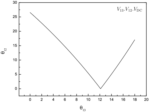
  Figure III.15: Case VDCll1. $\theta_{13}$ as a function of $\theta_{12}$ .

  We plot in Fig. III.15 $\theta_{23}$ as function of $\theta_{13}$, by setting $\theta_{23}$ its best fit value. It’s clear that we can not get the appropriate $\theta_{12}$ when $\theta_{13}$ changes in the range $[0^{\circ},~{}18^{\circ}]$ in this case. Such that it’s excluded. However, if we let $\theta_{23}$ changing in its $3\sigma$ range, a narrow appropriate parameter space of $\theta_{12}$ can be obtained. In short, this scenario doesn’t work for the best value.

• $\mathbf{VDC\ell\ell 2=V_{23}\cdot V_{12}\cdot V_{\rm DC}:}$ In this case we have

  $$\tan\theta_{12}=\left|{\sqrt{3}\cos x+\sin x\over\sqrt{3}\cos x-\sin x}\right|\;,$$ (94)

  $$\sin\theta_{13}=\left|{\sqrt{2\over 3}\sin x}\right|\;,$$ (95)

  $$\tan\theta_{23}=\left|{\sqrt{2}\cos x\cos y+\sin y\over\cos y-\sqrt{2}\cos x\sin y}\right|\;,$$ (96)

  The correlation between $\theta_{13}$ and $\theta_{12}$ is

  $$\sin\theta_{13}={1-\tan\theta_{12}\over\sqrt{2+2\tan^{2}\theta_{12}-2\tan\theta_{12}}}\;.$$ (97)

  We plot in the left panel of Fig. III.16, $\theta_{13}$ as function of $\theta_{12}$ and in the right panel of Fig. III.16 $\theta_{23}$ as function of y. We find that $\theta_{13}$ can only changes only in the range $[12.5^{\circ},~{}21.3^{\circ}]$. This range is excluded by the best fit value, but allowed by the T2K’s result. If future reactor neutrino oscillation experiments negate the T2K’s result, this scenario will be excluded definitely.

• $\mathbf{VDC\ell\ell 3=V_{23}\cdot V_{13}\cdot V_{\rm DC}:}$ The following equations can be obtained from this scenario

  $$\tan\theta_{12}=\left|{\sqrt{3}\cos z+\sqrt{2}\sin z\over\sqrt{3}\cos z-\sqrt{2}\sin z}\right|\;,$$ (98)

  $$\sin\theta_{13}=\left|{\sin z\over\sqrt{3}}\right|\;,$$ (99)

  $$\tan\theta_{23}=\left|{\sqrt{2}\cos y+\cos z\sin y\over\cos y\cos z-\sqrt{2}\sin y}\right|\;.$$ (100)

  We have

  $$\sin\theta_{13}={1-\tan\theta_{12}\over\sqrt{5\tan^{2}\theta_{12}-2\tan\theta_{12}+5}}\;.$$ (101)

  We plot in Fig.III.17 $\theta_{13}$ as function of $\theta_{12}$ and $\theta_{23}$ as function of y. It’s clear from the figure that $\theta_{13}$ can only change in the space $[6.4^{\circ},~{}10.5^{\circ}]$ in this scenario. We can get appropriate $\theta_{23}$ with big rotation angle $y$, which can be the result of certain flavor symmetry.

  

  

  Figure III.16: Case VDCll2. $\theta_{13}$ as a function of $\theta_{12}$ (left panel) and $\theta_{23}$ as a function of $y$ (right panel).

  

  

  Figure III.17: Case VDCll3. $\theta_{13}$ as a function of $\theta_{12}$ (left panel) and $\theta_{23}$ as a function of $y$ (right panel).

IV Summary

Among the knowns and unknowns of neutrino physics, the nonzero smallest lepton mixing angle $\theta_{13}$ has received a lot of attentions. The studying and measurement of $\theta_{13}$ is important to enrich our understanding of neutrino properties. Inspired by the recent T2K result of a relatively large $\theta_{13}$, We investigated some general modifications, which may minimal modifications or non-minimal modifications to the three well-known neutrino mixing pattern: Bimaximal, Tri-bimaximal and Democratic mixing patterns. Some non-trivial correlations between $\theta_{12}$, $\theta_{23}$ and $\theta_{13}$ were obtained. We investigated constraints on the $\theta_{13}$ by these correlations. Some modifications are already excluded by the current neutrino oscillation data, while the others give their predications on $\theta_{13}$. Future neutrino oscillation experiments may confirm or negate these models. Since $\theta_{13}$ is not so small, investigating leptonic CP-violating effects become relevant, but beyond the scope of this preliminary work. We will study this interesting and important topic somewhere else.

- (1) K. Nakamura et al., (Particle Data Group), J. Phys. G 37, 075021 (2010).
- (2) L. L. Chau and W. Y. Keung, Phys. Rev. Lett. 53, 1802 (1984).
- (3) M. Gonzales-Carcia, M. Maltoni and J. Salvado, arXiv:1001.4524; G. Fogli et al., J. Phys. Con. Ser, 203, 012103 (2010).
- (4) K. Abe et al., The T2K Collaboration, arXiv:1106.2822[hep-ex].
- (5) Z. Z. Xing, arXiv:1106.3244[hep-ph].
- (6) X. G. He and A. Zee, arXiv:1106.4359[hep-ph].
- (7) F. Vissani, hep-ph/9708483; V.D. Barger, S.Pakvasa, T.J. Weiler, and K. Whisnant, Phys. Lett. B437, 107 (1998); A.J. Baltz, A.S. Goldhaber, and M. Goldhaber, Phys. Rev. Lett. 81, 5730 (1998); I. Stancu and D.V. Ahluwalia, Phys. Lett. B460, 431 (1999); H. Georgi and S.L. Glashow, Phy. Rev. D61, 097301 (2000); N. Li and B.-Q. Ma, Phys. Lett. B 600, 248 (2004) [arXiv:hep-ph/0408235].
- (8) P.F. Harrison, D.H. Perkins, and W.G. Scott, Phys. Lett. B458, 79 (1999); Phys. Lett. B530, 167 (2002); Z.Z. Xing, Phys. Lett. B533, 85 (2002); P.F. Harrison and W.G. Scott, Phys. Lett. B535, 163 (2002); Phys. Lett. B557, 76 (2003); X.-G. He and A. Zee, Phys. Lett. B560, 87 (2003); See also L. Wolfenstein, Phys. Rev. D18, 958 (1978); Y. Yamanaka, H. Sugawara, and S. Pakvasa, Phys. Rev. D25, 1895 (1982); D29, 2135(E) (1984); N. Li and B.-Q. Ma, Phys. Rev. D 71, 017302 (2005) [arXiv:hep-ph/0412126].
- (9) H. Fritzsch and Z. Z. Xing, Phys. Lett. B 372, 265 (1996); Phys. Lett. B 440, 313 (1998); Phys. Rev. D 61,073016 (2000).
- (10) Y. J. Zheng and B. Q. Ma, arXiv:1106.4040[hep-ph].
- (11) E. Ma and D. Wegman, arXiv:1106.4269[hep-ph].
- (12) S. Zhou, arXiv:1106.4808[hep-ph].
- (13) T. Araki, arXiv:1106.5211[hep-ph].
- (14) N. Haba, R. Takahashi, arXiv:1106.5926[hep-ph].
- (15) D. Meloni, arXiv:1107.0221[hep-ph].
- (16) S. N. Gninenko, arXiv:1107.0279[hep-ph].