Distributed Matrix Completion
and Robust Factorization

Abstract

If learning methods are to scale to the massive sizes of modern datasets, it is essential for the field of machine learning to embrace parallel and distributed computing. Inspired by the recent development of matrix factorization methods with rich theory but poor computational complexity and by the relative ease of mapping matrices onto distributed architectures, we introduce a scalable divide-and-conquer framework for noisy matrix factorization. We present a thorough theoretical analysis of this framework in which we characterize the statistical errors introduced by the “divide” step and control their magnitude in the “conquer” step, so that the overall algorithm enjoys high-probability estimation guarantees comparable to those of its base algorithm. We also present experiments in collaborative filtering and video background modeling that demonstrate the near-linear to superlinear speed-ups attainable with this approach.

^a Department of Statistics, Stanford
^b Department of Engineering and Computer Science, UC Berkeley
^c Department of Statistics, UC Berkeley
^$\dagger$ These authors contributed equally.

1 Introduction

The scale of modern scientific and technological datasets poses major new challenges for computational and statistical science. Data analyses and learning algorithms suitable for modest-sized datasets are often entirely infeasible for the terabyte and petabyte datasets that are fast becoming the norm. There are two basic responses to this challenge. One response is to abandon algorithms that have superlinear complexity, focusing attention on simplified algorithms that—in the setting of massive data—may achieve satisfactory results because of the statistical strength of the data. While this is a reasonable research strategy, it requires developing suites of algorithms of varying computational complexity for each inferential task and calibrating statistical and computational efficiencies. There are many open problems that need to be solved if such an effort is to bear fruit.

The other response to the massive data problem is to retain existing algorithms but to apply them to subsets of the data. To obtain useful results under this approach, one embraces parallel and distributed computing architectures, applying existing base algorithms to multiple subsets of the data in parallel and then combining the results. Such a divide-and-conquer methodology has two main virtues: (1) it builds directly on algorithms that have proven their value at smaller scales and that often have strong theoretical guarantees, and (2) it requires little in the way of new algorithmic development. The major challenge, however, is in preserving the theoretical guarantees of the base algorithm once one embeds the algorithm in a computationally-motivated divide-and-conquer procedure. Indeed, the theoretical guarantees often refer to subtle statistical properties of the data-generating mechanism (e.g., sparsity, information spread, and near low-rankedness). These may or may not be retained under the “divide” step of a putative divide-and-conquer solution. In fact, we generally would expect subsampling operations to damage the relevant statistical structures. Even if these properties are preserved, we face the difficulty of combining the intermediary results of the “divide” step into a final consilient solution to the original problem. The question, therefore, is whether we can design divide-and-conquer algorithms that manage the tradeoffs relating these statistical properties to the computational degrees of freedom such that the overall algorithm provides a scalable solution that retains the theoretical guarantees of the base algorithm.

In this paper, we explore this issue in the context of an important class of machine learning algorithms—the matrix factorization algorithms underlying a wide variety of practical applications, including collaborative filtering for recommender systems (e.g., [22] and the references therein), link prediction for social networks [17], click prediction for web search [6], video surveillance [2], graphical model selection [4], document modeling [31], and image alignment [37]. We focus on two instances of the general matrix factorization problem: noisy matrix completion [3], where the goal is to recover a low-rank matrix from a small subset of noisy entries, and noisy robust matrix factorization [2, 4], where the aim is to recover a low-rank matrix from corruption by noise and outliers of arbitrary magnitude. These two classes of matrix factorization problems have attracted significant interest in the research community.

Various approaches have been proposed for scalable noisy matrix factorization problems, in particular for noisy matrix completion, though the vast majority tackle rank-constrained non-convex formulations of these problems with no assurance of finding optimal solutions [47, 12, 39, 10, 46]. In contrast, convex formulations of noisy matrix factorization relying on the nuclear norm have been shown to admit strong theoretical estimation guarantees [1, 2, 3, 34], and a variety of algorithms [e.g., 27, 28, 42] have been developed for solving both matrix completion and robust matrix factorization via convex relaxation. Unfortunately, however, all of these methods are inherently sequential, and all rely on the repeated and costly computation of truncated singular value decompositions (SVDs), factors that severely limit the scalability of the algorithms. Moreover, previous attempts at reducing this computational burden have introduced approximations without theoretical justification [33].

To address this key problem of noisy matrix factorization in a scalable and theoretically sound manner, we propose a divide-and-conquer framework for large-scale matrix factorization. Our framework, entitled Divide-Factor-Combine (DFC), randomly divides the original matrix factorization task into cheaper subproblems, solves those subproblems in parallel using a base matrix factorization algorithm for nuclear norm regularized formulations, and combines the solutions to the subproblems using efficient techniques from randomized matrix approximation. We develop a thoroughgoing theoretical analysis for the DFC framework, linking statistical properties of the underlying matrix to computational choices in the algorithms and thereby providing conditions under which statistical estimation of the underlying matrix is possible. We also present experimental results for several DFC variants demonstrating that DFC can provide near-linear to superlinear speed-ups in practice.

The remainder of the paper is organized as follows. In Sec. 2, we define the setting of noisy matrix factorization and introduce the components of the DFC framework. Secs. 3, 4, and 5 present our theoretical analysis of DFC, along with a new analysis of convex noisy matrix completion and a novel characterization of randomized matrix approximation algorithms. To illustrate the practical speed-up and robustness of DFC, we present experimental results on collaborative filtering, video background modeling, and simulated data in Sec. 6. Finally, we conclude in Sec. 7.

Notation

For a matrix ${\mathbf{M}}\in\mathbb{R}^{m\times n}$, we define ${\mathbf{M}}_{(i)}$ as the $i$th row vector, ${\mathbf{M}}^{(j)}$ as the $j$th column vector, and ${\mathbf{M}}_{ij}$ as the $ij$th entry. If $\mathrm{rank}({{\mathbf{M}}})=r$, we write the compact singular value decomposition (SVD) of ${\mathbf{M}}$ as ${\mathbf{U}}_{M}{\mathbf{\Sigma}}_{M}{\mathbf{V}}_{M}^{\top}$, where ${\mathbf{\Sigma}}_{M}$ is diagonal and contains the $r$ non-zero singular values of ${\mathbf{M}}$, and ${\mathbf{U}}_{M}\in\mathbb{R}^{m\times r}$ and ${\mathbf{V}}_{M}\in\mathbb{R}^{n\times r}$ are the corresponding left and right singular vectors of ${\mathbf{M}}$. We define ${\mathbf{M}}^{+}={\mathbf{V}}_{M}{\mathbf{\Sigma}}_{M}^{-1}{\mathbf{U}}_{M}^{\top}$ as the Moore-Penrose pseudoinverse of ${\mathbf{M}}$ and ${\mathbf{P}}_{M}={\mathbf{M}}{\mathbf{M}}^{+}$ as the orthogonal projection onto the column space of ${\mathbf{M}}$. We let ${\|{\cdot}\|}_{2}$, ${\|{\cdot}\|}_{F}$, and ${\|{\cdot}\|}_{*}$ respectively denote the spectral, Frobenius, and nuclear norms of a matrix, ${\|{\cdot}\|}_{\infty}$ denote the maximum entry of a matrix, and ${\|{\cdot}\|}$ represent the $\ell_{2}$ norm of a vector.

2 The Divide-Factor-Combine Framework

In this section, we present a general divide-and-conquer framework for scalable noisy matrix factorization. We begin by defining the problem setting of interest.

2.1 Noisy Matrix Factorization (MF)

In the setting of noisy matrix factorization, we observe a subset of the entries of a matrix ${\mathbf{M}}={\mathbf{L}}_{0}+{\mathbf{S}}_{0}+{\mathbf{Z}}_{0}\in\mathbb{R}^{m\times n}$, where ${\mathbf{L}}_{0}$ has rank $r\ll m,n$, ${\mathbf{S}}_{0}$ represents a sparse matrix of outliers of arbitrary magnitude, and ${\mathbf{Z}}_{0}$ is a dense noise matrix. We let ${\Omega}$ represent the locations of the observed entries and ${\mathcal{P}}_{{\Omega}}$ be the orthogonal projection onto the space of $m\times n$ matrices with support ${\Omega}$, so that

$$({\mathcal{P}}_{{\Omega}}({\mathbf{M}}))_{ij}={\mathbf{M}}_{ij},\ \text{if}\ (i,j)\in\Omega\quad\text{and}\quad({\mathcal{P}}_{{\Omega}}({\mathbf{M}}))_{ij}=0\ \text{otherwise}.$$

Our goal is to estimate the low-rank matrix ${\mathbf{L}}_{0}$ from ${\mathcal{P}}_{{\Omega}}({\mathbf{M}})$ with error proportional to the noise level $\Delta\triangleq{\|{{\mathbf{Z}}_{0}}\|}_{F}$. We will focus on two specific instances of this general problem:

• Noisy Matrix Completion (MC): $s\triangleq|{\Omega}|$ entries of ${\mathbf{M}}$ are revealed uniformly without replacement, along with their locations. There are no outliers, so that ${\mathbf{S}}_{0}$ is identically zero.

• Noisy Robust Matrix Factorization (RMF): ${\mathbf{S}}_{0}$ is identically zero save for $s$ outlier entries of arbitrary magnitude with unknown locations distributed uniformly without replacement. All entries of ${\mathbf{M}}$ are observed, so that ${\mathcal{P}}_{{\Omega}}({\mathbf{M}})={\mathbf{M}}$.

2.2 Divide-Factor-Combine

The Divide-Factor-Combine (DFC) framework divides the expensive task of matrix factorization into smaller subproblems, executes those subproblems in parallel, and then efficiently combines the results into a final low-rank estimate of ${\mathbf{L}}_{0}$. We highlight three variants of this general framework in Algorithms 1, 2, and 3. These algorithms, which we refer to as DFC-Proj, DFC-RP, and DFC-Nys, differ in their strategies for division and recombination but adhere to a common pattern of three simple steps:

(D step)

Divide input matrix into submatrices: DFC-Proj and DFC-RP randomly partition ${\mathcal{P}}_{{\Omega}}({\mathbf{M}})$ into $t$ $l$-column submatrices, $\{{\mathcal{P}}_{{\Omega}}({\mathbf{C}}_{1}),\ldots,{\mathcal{P}}_{{\Omega}}({\mathbf{C}}_{t})\}$, while DFC-Nys selects an $l$-column submatrix, ${\mathcal{P}}_{{\Omega}}({\mathbf{C}})$, and a $d$-row submatrix, ${\mathcal{P}}_{{\Omega}}({\mathbf{R}})$, uniformly at random.

(F step)

Factor each submatrix in parallel using any base MF algorithm: DFC-Proj and DFC-RP perform $t$ parallel submatrix factorizations, while DFC-Nys performs two such parallel factorizations. Standard base MF algorithms output the following low-rank approximations: $\{\hat{\mathbf{C}}_{1},\ldots,\hat{\mathbf{C}}_{t}\}$ for DFC-Proj and DFC-RP; $\hat{\mathbf{C}}$ and $\hat{\mathbf{R}}$ for DFC-Nys. All matrices are retained in factored form.

(C step)

Combine submatrix estimates: DFC-Proj generates a final low-rank estimate ${\hat{{\mathbf{L}}}^{proj}}$ by projecting $[\hat{\mathbf{C}}_{1},\ldots,\hat{\mathbf{C}}_{t}]$ onto the column space of $\hat{\mathbf{C}}_{1}$, DFC-RP uses random projection to compute a rank-$k$ estimate ${\hat{{\mathbf{L}}}^{rp}}$ of $[\hat{\mathbf{C}}_{1}\cdots\hat{\mathbf{C}}_{t}]$ where $k$ is the median rank of the returned subproblem estimates, and DFC-Nys forms the low-rank estimate ${\hat{{\mathbf{L}}}^{nys}}$ from $\hat{\mathbf{C}}$ and $\hat{\mathbf{R}}$ via the generalized Nyström method. These matrix approximation techniques are described in more detail in Sec. 2.3.

Algorithm 1 DFC-Proj

  Input: ${\mathcal{P}}_{{\Omega}}({\mathbf{M}})$, $t$

  $\{{\mathcal{P}}_{{\Omega}}({\mathbf{C}}_{i})\}_{1\leq i\leq t}$ = SampCol(${\mathcal{P}}_{{\Omega}}({\mathbf{M}})$, $t)$ do in parallel

        $\hat{{\mathbf{C}}}_{1}$ = Base-MF-Alg$({\mathcal{P}}_{{\Omega}}({\mathbf{C}}_{1}))$

                             ⋮

        $\hat{{\mathbf{C}}}_{t}$ = Base-MF-Alg$({\mathcal{P}}_{{\Omega}}({\mathbf{C}}_{t}))$end do

  ${\hat{{\mathbf{L}}}^{proj}}$ = ColProjection($\hat{{\mathbf{C}}}_{1},\ldots,\hat{{\mathbf{C}}}_{t})$

Algorithm 2 DFC-RP

  Input: ${\mathcal{P}}_{{\Omega}}({\mathbf{M}})$, $t$

  $\{{\mathcal{P}}_{{\Omega}}({\mathbf{C}}_{i})\}_{1\leq i\leq t}$ = SampCol(${\mathcal{P}}_{{\Omega}}({\mathbf{M}})$, $t)$ do in parallel

        $\hat{{\mathbf{C}}}_{1}$ = Base-MF-Alg$({\mathcal{P}}_{{\Omega}}({\mathbf{C}}_{1}))$

                             ⋮

        $\hat{{\mathbf{C}}}_{t}$ = Base-MF-Alg$({\mathcal{P}}_{{\Omega}}({\mathbf{C}}_{t}))$end do

  $k=\text{median}_{i\in\{1\ldots t\}}\big{(}\text{rank}(\hat{\mathbf{C}}_{i})\big{)}$

  ${\hat{{\mathbf{L}}}^{proj}}$ = RandProjection($\hat{{\mathbf{C}}}_{1},\ldots,\hat{{\mathbf{C}}}_{t},k)$

Algorithm 3 DFC-Nys

  Input: ${\mathcal{P}}_{{\Omega}}({\mathbf{M}})$, $l$, $d$

  ${\mathcal{P}}_{{\Omega}}({\mathbf{C}})\,,{\mathcal{P}}_{{\Omega}}({\mathbf{R}})$ = SampColRow(${\mathcal{P}}_{{\Omega}}({\mathbf{M}})$, $l$, $d)$ do in parallel

        $\hat{{\mathbf{C}}}$ = Base-MF-Alg$({\mathcal{P}}_{{\Omega}}({\mathbf{C}}))$

        $\hat{{\mathbf{R}}}$ = Base-MF-Alg$({\mathcal{P}}_{{\Omega}}({\mathbf{R}}))$end do

  ${\hat{{\mathbf{L}}}^{nys}}$ = GenNyström($\hat{{\mathbf{C}}}$, $\hat{{\mathbf{R}}})$

2.3 Randomized Matrix Approximations

Underlying the C step of each DFC algorithm is a method for generating randomized low-rank approximations to an arbitrary matrix ${\mathbf{M}}$.

Column Projection

DFC-Proj (Algorithm 1) uses the column projection method of Frieze et al. [11]. Suppose that ${\mathbf{C}}$ is a matrix of $l$ columns sampled uniformly and without replacement from the columns of ${\mathbf{M}}$. Then, column projection generates a “matrix projection” approximation [23] of ${\mathbf{M}}$ via

$${\mathbf{L}}^{proj}={\mathbf{C}}{\mathbf{C}}^{+}{\mathbf{M}}={\mathbf{U}}_{C}{\mathbf{U}}_{C}^{\top}{\mathbf{M}}.$$ (1)

In practice, we do not reconstruct ${\mathbf{L}}^{proj}$ but rather maintain low-rank factors, e.g., ${\mathbf{U}}_{C}$ and ${\mathbf{U}}_{C}^{\top}{\mathbf{M}}$.

Random Projection

The celebrated result of Johnson and Lindenstrauss [20] shows that random low-dimensional embeddings preserve Euclidean geometry. Inspired by this result, several random projection algorithms [e.g., 36, 25, 40] have been introduced for approximating a matrix by projecting it onto a random low-dimensional subspace (see Halko et al. [15] for further discussion). DFC-RP (Algorithm 2) utilizes such a random projection method due to Halko et al. [15]. Given a target low-rank parameter $k$, let ${\mathbf{G}}$ be an $n\times(k+p)$ standard Gaussian matrix ${\mathbf{G}}$, where $p$ is an oversampling parameter. Next, let ${\mathbf{Y}}=({\mathbf{M}}{\mathbf{M}}^{\top})^{q}{\mathbf{M}}{\mathbf{G}}$, and define ${\mathbf{Q}}\in\mathbb{R}^{m\times k}$ as the top $k$ left singular vectors of ${\mathbf{Y}}$. The random projection approximation of ${\mathbf{M}}$ is then given by

$${\mathbf{L}}^{rp}={\mathbf{Q}}{\mathbf{Q}}^{+}{\mathbf{M}}.$$ (2)

We work with an implementation [43] of a numerically stable variant of this algorithm described in Algorithm $4.4$ of Halko et al. [15]. Moreover, the parameters $p$ and $q$ are typically set to small positive constants [43, 15], and we set $p=5$ and $q=2$.

Generalized Nyström Method

The Nyström method was developed for the discretization of integral equations [35] and has since been used to speed up large-scale learning applications involving symmetric positive semidefinite matrices [45]. DFC-Nys (Algorithm 3) makes use of a generalization of the Nyström method for arbitrary real matrices [13]. Suppose that ${\mathbf{C}}$ consists of $l$ columns of ${\mathbf{M}}$, sampled uniformly without replacement, and that ${\mathbf{R}}$ consists of $d$ rows of ${\mathbf{M}}$, independently sampled uniformly and without replacement. Let ${\mathbf{W}}$ be the $d\times l$ matrix formed by sampling the corresponding rows of ${\mathbf{C}}$. Then, the generalized Nyström method computes a “spectral reconstruction” approximation [23] of ${\mathbf{M}}$ via

$${\mathbf{L}}^{nys}={\mathbf{C}}{\mathbf{W}}^{+}{\mathbf{R}}={\mathbf{C}}{\mathbf{V}}_{W}{\mathbf{\Sigma}}_{W}^{+}{\mathbf{U}}_{W}^{\top}{\mathbf{R}}\,.$$ (3)

As with ${\mathbf{M}}^{proj}$, we store low-rank factors of ${\mathbf{L}}^{nys}$, such as ${\mathbf{C}}{\mathbf{V}}_{W}{\mathbf{\Sigma}}_{W}^{+}$ and ${\mathbf{U}}_{W}^{\top}{\mathbf{R}}$.

2.4 Running Time of DFC

Many state-of-the-art MF algorithms have $\Omega(mnk_{M})$ per-iteration time complexity due to the rank-$k_{M}$ truncated SVD performed on each iteration. DFC significantly reduces the per-iteration complexity to O$(mlk_{C_{i}})$ time for ${\mathbf{C}}_{i}$ (or ${\mathbf{C}}$) and O$(ndk_{R})$ time for ${\mathbf{R}}$. The cost of combining the submatrix estimates is even smaller when using column projection or the generalized Nyström method, since the outputs of standard MF algorithms are returned in factored form. Indeed, if we define $k^{\prime}\triangleq\max_{i}k_{C_{i}}$, then the column projection step of DFC-Proj requires only O$(mk^{\prime 2}+lk^{\prime 2})$ time: O$(mk^{\prime 2}+lk^{\prime 2})$ time for the pseudoinversion of $\hat{\mathbf{C}}_{1}$ and O$(mk^{\prime 2}+lk^{\prime 2})$ time for matrix multiplication with each $\hat{\mathbf{C}}_{i}$ in parallel. Similarly, the generalized Nyström step of DFC-Nys requires only O$(l\bar{k}^{2}+d\bar{k}^{2}+\min\mathopen{}\mathclose{{}\left({m,n}}\right)\bar{k}^{2})$ time, where $\bar{k}\triangleq\max\mathopen{}\mathclose{{}\left({k_{C},k_{R}}}\right)$.

DFC-RP also benefits from the factored form of the outputs of standard MF algorithms. Assuming that $p$ and $q$ are positive constants, the random projection step of DFC-RP requires O($mkt+mkk^{\prime}+nk$) time where $k$ is the low-rank parameter of ${\mathbf{Q}}$: O($nk$) time to generate ${\mathbf{G}}$, O($mkk^{\prime}+mkt$) to compute ${\mathbf{Y}}$ in parallel, O($mk^{2}$) to compute the SVD of ${\mathbf{Y}}$, and O$(mk^{\prime 2}+lk^{\prime 2})$ time for matrix multiplication with each $\hat{\mathbf{C}}_{i}$ in parallel in the final projection step. Note that the running time of the random projection step depends on $t$ (even when executed in parallel) and thus has a larger complexity than the column projection and generalized Nyström variants. Nevertheless, the random projection step need be performed only once and thus yields a significant savings over the repeated computation of SVDs required by typical base algorithms.

2.5 Ensemble Methods

Ensemble methods have been shown to improve performance of matrix approximation algorithms, while straightforwardly leveraging the parallelism of modern many-core and distributed architectures [24]. As such, we propose ensemble variants of the DFC algorithms that demonstrably reduce estimation error while introducing a negligible cost to the parallel running time. For DFC-Proj-Ens, rather than projecting only onto the column space of $\hat{\mathbf{C}}_{1}$, we project $[\hat{\mathbf{C}}_{1},\ldots,\hat{\mathbf{C}}_{t}]$ onto the column space of each $\hat{\mathbf{C}}_{i}$ in parallel and then average the $t$ resulting low-rank approximations. For DFC-RP-Ens, rather than projecting only onto a column space derived from a single random matrix ${\mathbf{G}}$, we project $[\hat{\mathbf{C}}_{1},\ldots,\hat{\mathbf{C}}_{t}]$ onto $t$ column spaces derived from $t$ random matrices in parallel and then average the $t$ resulting low-rank approximations. For DFC-Nys-Ens, we choose a random $d$-row submatrix ${\mathcal{P}}_{{\Omega}}({\mathbf{R}})$ as in DFC-Nys and independently partition the columns of ${\mathcal{P}}_{{\Omega}}({\mathbf{M}})$ into $\{{\mathcal{P}}_{{\Omega}}({\mathbf{C}}_{1}),\ldots,{\mathcal{P}}_{{\Omega}}({\mathbf{C}}_{t})\}$ as in DFC-Proj and DFC-RP. After running the base MF algorithm on each submatrix, we apply the generalized Nyström method to each $(\hat{\mathbf{C}}_{i},\hat{\mathbf{R}})$ pair in parallel and average the $t$ resulting low-rank approximations. Sec. 6 highlights the empirical effectiveness of ensembling.

3 Roadmap of Theoretical Analysis

While DFC in principle can work with any base matrix factorization algorithm, it offers the greatest benefits when united with accurate but computationally expensive base procedures. Convex optimization approaches to matrix completion and robust matrix factorization [e.g., 27, 28, 42] are prime examples of this class, since they admit strong theoretical estimation guarantees [1, 2, 3, 34] but suffer from poor computational complexity due to the repeated and costly computation of truncated SVDs. Sec. 6 will provide empirical evidence that DFC provides an attractive framework to improve the scalability of these algorithms, but we first present a thorough theoretical analysis of the estimation properties of DFC.

Over the course of the next three sections, we will show that the same assumptions that give rise to strong estimation guarantees for standard MF formulations also guarantee strong estimation properties for DFC. In the remainder of this section, we first introduce these standard assumptions and then present simplified bounds to build intuition for our theoretical results and our underlying proof techniques.

3.1 Standard Assumptions for Noisy Matrix Factorization

Since not all matrices can be recovered from missing entries or gross outliers, recent theoretical advances have studied sufficient conditions for accurate noisy MC [3, 21, 34] and RMF [1, 48]. Informally, these conditions capture the degree to which information about a single entry is “spread out” across a matrix. The ease of matrix estimation is correlated with this spread of information. The most prevalent set of conditions are matrix coherence conditions, which limit the extent to which the singular vectors of a matrix are correlated with the standard basis. However, there exist classes of matrices that violate the coherence conditions but can nonetheless be recovered from missing entries or gross outliers. Negahban and Wainwright [34] define an alternative notion of matrix spikiness in part to handle these classes.

3.1.1 Matrix Coherence

Letting ${\mathbf{e}}_{i}$ be the $i$th column of the standard basis, we define two standard notions of coherence [38]:

Definition 1 ($\mu_{0}$-Coherence).

Let ${\mathbf{V}}\in\mathbb{R}^{n\times r}$ contain orthonormal columns with $r\leq n$. Then the $\mu_{0}$-coherence of ${\mathbf{V}}$ is:

$$\textstyle\mu_{0}({\mathbf{V}})\triangleq\frac{n}{r}\max_{1\leq i\leq n}{\|{{\mathbf{P}}_{V}{\mathbf{e}}_{i}}\|}^{2}=\frac{n}{r}\max_{1\leq i\leq n}{\|{{\mathbf{V}}_{(i)}}\|}^{2}\,.$$

Definition 2 ($\mu_{1}$-Coherence).

Let ${\mathbf{L}}\in\mathbb{R}^{m\times n}$ have rank $r$. Then, the $\mu_{1}$-coherence of ${\mathbf{L}}$ is:

$$\textstyle\mu_{1}({\mathbf{L}})\triangleq\sqrt{\frac{mn}{r}}\max_{ij}|{\mathbf{e}}_{i}^{\top}{\mathbf{U}}_{L}{\mathbf{V}}_{L}^{\top}{\mathbf{e}}_{j}|\,.$$

For conciseness, we extend the definition of $\mu_{0}$-coherence to an arbitrary matrix ${\mathbf{L}}\in\mathbb{R}^{m\times n}$ with rank $r$ via $\mu_{0}({\mathbf{L}})\triangleq\max\mathopen{}\mathclose{{}\left({\mu_{0}({\mathbf{U}}_{L}),\mu_{0}({\mathbf{V}}_{L})}}\right).$ Further, for any $\mu>0$, we will call a matrix ${\mathbf{L}}$ $(\mu,r)$-coherent if $\mathrm{rank}({{\mathbf{L}}})=r$, $\mu_{0}({\mathbf{L}})\leq\mu$, and $\mu_{1}({\mathbf{L}})\leq\sqrt{\mu}$. Our analysis in Sec. 4 will focus on base MC and RMF algorithms that express their estimation guarantees in terms of the $(\mu,r)$-coherence of the target low-rank matrix ${\mathbf{L}}_{0}$. For such algorithms, lower values of $\mu$ correspond to better estimation properties.

3.1.2 Matrix Spikiness

The matrix spikiness condition of Negahban and Wainwright [34] captures the intuition that a matrix is easier to estimate if its maximum entry is not much larger than its average entry (in the root mean square sense):

Definition 3 (Spikiness).

The spikiness of ${\mathbf{L}}\in\mathbb{R}^{m\times n}$ is:

$$\textstyle\alpha({\mathbf{L}})\triangleq\sqrt{mn}{\|{{\mathbf{L}}}\|}_{\infty}/{\|{{\mathbf{L}}}\|}_{F}.$$

We call a matrix $\alpha$-spiky if $\alpha({\mathbf{L}})\leq\alpha$.

Our analysis in Sec. 5 will focus on base MC algorithms that express their estimation guarantees in terms of the $\alpha$-spikiness of the target low-rank matrix ${\mathbf{L}}_{0}$. For such algorithms, lower values of $\alpha$ correspond to better estimation properties.

3.2 Prototypical Estimation Bounds

We now present a prototypical estimation bound for DFC. Suppose that a base MC algorithm solves the noisy nuclear norm heuristic, studied in Candès and Plan [3]:

$$\text{minimize}_{{\mathbf{L}}}\quad{\|{{\mathbf{L}}}\|}_{*}\quad\text{subject\, to}\quad{\|{{\mathcal{P}}_{{\Omega}}({\mathbf{M}}-{\mathbf{L}})}\|}_{F}\leq\Delta,$$

and that, for simplicity, ${\mathbf{M}}$ is square. The following prototype bound, derived from a new noisy MC guarantee in Thm. 10, describes the behavior of this estimator under matrix coherence assumptions. Note that the bound implies exact recovery in the noiseless setting, i.e., when $\Delta=0$.

Proto-Bound 1 (MC under Incoherence).

Suppose that ${\mathbf{L}}_{0}$ is $(\mu,r)$-coherent, $s$ entries of ${\mathbf{M}}\in\mathbb{R}^{n\times n}$ are observed uniformly at random where $s=\Omega(\mu rn\log^{2}(n))$, and ${\|{{\mathbf{M}}-{\mathbf{L}}_{0}}\|}_{F}\leq\Delta$. If $\hat{\mathbf{L}}$ solves the noisy nuclear norm heuristic, then

$${\|{{\mathbf{L}}_{0}-\hat{\mathbf{L}}}\|}_{F}\leq f(n)\Delta$$

with high probability, where $f$ is a function of $n$.

Now we present a corresponding prototype bound for DFC-Proj, a simplified version of our Cor. 13, under precisely the same coherence assumptions. Notably, this bound i) preserves accuracy with a flexible $(2+\epsilon)$ degradation in estimation error over the base algorithm, ii) allows for speed-up by requiring only a vanishingly small fraction of columns to be sampled (i.e., $l/n\rightarrow 0$) whenever $s=\omega(n\log^{2}(n))$ entries are revealed, and iii) maintains exact recovery in the noiseless setting.

Proto-Bound 2 (DFC-MC under Incoherence).

Suppose that ${\mathbf{L}}_{0}$ is $(\mu,r)$-coherent, $s$ entries of ${\mathbf{M}}\in\mathbb{R}^{n\times n}$ are observed uniformly at random, and ${\|{{\mathbf{M}}-{\mathbf{L}}_{0}}\|}_{F}\leq\Delta$. Then

$$l=O\bigg{(}\frac{\mu^{2}r^{2}n^{2}\log^{2}(n)}{s\epsilon^{2}}\bigg{)}$$

random columns suffice to have

$${\|{{\mathbf{L}}_{0}-{\hat{{\mathbf{L}}}^{proj}}}\|}_{F}\leq(2+\epsilon)f(n)\Delta$$

with high probability when the noisy nuclear norm heuristic is used as a base algorithm, where $f$ is the same function of $n$ defined in Proto. 1.

The proof of Proto. 2, and indeed of each of our main DFC results, consists of three high-level steps:

1. Bound information spread of submatrices: Recall that the F step of DFC operates by applying a base MF algorithm to submatrices. We show that, with high probability, uniformly sampled submatrices are only moderately more coherent and moderately more spiky than the matrix from which they are drawn. This allows for accurate estimation of submatrices using base algorithms with standard coherence or spikiness requirements. The conservation of incoherence result is summarized in Lem. 4, while the conservation of non-spikiness is presented in Lem. 15.

2. Bound error of randomized matrix approximations: The error introduced by the C step of DFC depends on the framework variant. Drawing upon tools from randomized $\ell_{2}$ regression [9], randomized matrix multiplication [7, 8], and matrix concentration [19], we show that the same assumptions on the spread of information responsible for accurate MC and RMF also yield high fidelity reconstructions for column projection (Cor. 6 and Thm. 16) and the Nyström method (Cor. 7 and Cor. 8). We additionally present general approximation guarantees for random projection due to Halko et al. [15] in Cor. 9. These results give rise to “master theorems” for coherence (Thm. 12) and spikiness (Thm. 18) that generically relate the estimation error of DFC to the error of any base algorithm.

3. Bound error of submatrix factorizations: The final step combines a master theorem with a base estimation guarantee applied to each DFC subproblem. We study both new (Thm. 10) and established bounds (Thm. 11 and Cor. 17) for MC and RMF and prove that DFC submatrices satisfy the base guarantee preconditions with high probability. We present the resulting coherence-based estimation guarantees for DFC in Cor. 13 and Cor. 14 and the spikiness-based estimation guarantee in Cor. 19.

The next two sections present the main results contributing to each of these proof steps, as well as their consequences for MC and RMF. Sec. 4 presents our analysis under coherence assumptions, while Sec. 5 contains our spikiness analysis.

4 Coherence-based Theoretical Analysis

4.1 Coherence Analysis of Randomized Approximation Algorithms

We begin our coherence-based analysis by characterizing the behavior of randomized approximation algorithms under standard coherence assumptions. The derived properties will aid us in deriving DFC estimation guarantees. Hereafter, $\epsilon\in(0,1]$ represents a prescribed error tolerance, and $\delta,\delta^{\prime}\in(0,1]$ denote target failure probabilities.

4.1.1 Conservation of Incoherence

Our first result bounds the $\mu_{0}$ and $\mu_{1}$-coherence of a uniformly sampled submatrix in terms of the coherence of the full matrix. This conservation of incoherence allows for accurate submatrix completion or submatrix outlier removal when using standard MC and RMF algorithms. Its proof is given in Sec. B.

Lemma 4 (Conservation of Incoherence).

Let ${\mathbf{L}}\in\mathbb{R}^{m\times n}$ be a rank-$r$ matrix and define ${\mathbf{L}}_{C}\in\mathbb{R}^{m\times l}$ as a matrix of $l$ columns of ${\mathbf{L}}$ sampled uniformly without replacement. If $l\geq cr\mu_{0}({\mathbf{V}}_{L})\log(n)\log(1/\delta)/\epsilon^{2},$ where $c$ is a fixed positive constant defined in Cor. 6, then

1. $\mathrm{rank}({{\mathbf{L}}_{C}})=\mathrm{rank}({{\mathbf{L}}})$

2. $\mu_{0}({\mathbf{U}}_{L_{C}})=\mu_{0}({\mathbf{U}}_{L})$

3. $\displaystyle\mu_{0}({\mathbf{V}}_{L_{C}})\leq\frac{\mu_{0}({\mathbf{V}}_{L})}{1-\epsilon/2}$

4. $\displaystyle\mu_{1}^{2}({\mathbf{L}}_{C})\leq\frac{r\mu_{0}({\mathbf{U}}_{L})\mu_{0}({\mathbf{V}}_{L})}{1-\epsilon/2}$

all hold jointly with probability at least $1-\delta/n$.

4.1.2 Column Projection Analysis

Our next result shows that projection based on uniform column sampling leads to near optimal estimation in matrix regression when the covariate matrix has small coherence. This statement will immediately give rise to estimation guarantees for column projection and the generalized Nyström method.

Theorem 5 (Subsampled Regression under Incoherence).

Given a target matrix ${\mathbf{B}}\in\mathbb{R}^{p\times n}$ and a rank-$r$ matrix of covariates ${\mathbf{L}}\in\mathbb{R}^{m\times n}$, choose $l\geq 3200r\mu_{0}({\mathbf{V}}_{L})\log(4n/\delta)/\epsilon^{2},$ let ${\mathbf{B}}_{C}\in\mathbb{R}^{p\times l}$ be a matrix of $l$ columns of ${\mathbf{B}}$ sampled uniformly without replacement, and let ${\mathbf{L}}_{C}\in\mathbb{R}^{m\times l}$ consist of the corresponding columns of ${\mathbf{L}}$. Then,

$${\|{{\mathbf{B}}-{\mathbf{B}}_{C}{\mathbf{L}}_{C}^{+}{\mathbf{L}}}\|}_{F}\leq(1+\epsilon){\|{{\mathbf{B}}-{\mathbf{B}}{\mathbf{L}}^{+}{\mathbf{L}}}\|}_{F}$$

with probability at least $1-\delta-0.2$.

Fundamentally, Thm. 5 links the notion of coherence, common in matrix estimation communities, to the randomized approximation concept of leverage score sampling  [30]. The proof of Thm. 5, given in Sec. A, builds upon the randomized $\ell_{2}$ regression work of Drineas et al. [9] and the matrix concentration results of Hsu et al. [19] to yield a subsampled regression guarantee with better sampling complexity than that of Drineas et al. [9, Thm. 5].

A first consequence of Thm. 5 shows that, with high probability, column projection produces an estimate nearly as good as a given rank-$r$ target by sampling a number of columns proportional to the coherence and $r\log n$.

Corollary 6 (Column Projection under Incoherence).

Given a matrix ${\mathbf{M}}\in\mathbb{R}^{m\times n}$ and a rank-$r$ approximation ${\mathbf{L}}\in\mathbb{R}^{m\times n}$, choose $l\geq cr\mu_{0}({\mathbf{V}}_{L})\log(n)\log(1/\delta)/\epsilon^{2},$ where $c$ is a fixed positive constant, and let ${\mathbf{C}}\in\mathbb{R}^{m\times l}$ be a matrix of $l$ columns of ${\mathbf{M}}$ sampled uniformly without replacement. Then,

$${\|{{\mathbf{M}}-{\mathbf{C}}{\mathbf{C}}^{+}{\mathbf{M}}}\|}_{F}\leq(1+\epsilon){\|{{\mathbf{M}}-{\mathbf{L}}}\|}_{F}$$

with probability at least $1-\delta$.

Our result generalizes Thm. 1 of Drineas et al. [9] by providing improved sampling complexity and guarantees relative to an arbitrary low-rank approximation. Notably, in the “noiseless” setting, when ${\mathbf{M}}={\mathbf{L}}$, Cor. 6 guarantees exact recovery of ${\mathbf{M}}$ with high probability. The proof of Cor. 6 is given in Sec. C.

4.1.3 Generalized Nyström Analysis

Thm. 5 and Cor. 6 together imply an estimation guarantee for the generalized Nyström method relative to an arbitrary low-rank approximation ${\mathbf{L}}$. Indeed, if the matrix of sampled columns is denoted by ${\mathbf{C}}$, then, with appropriately reduced probability, O($\mu_{0}({\mathbf{V}}_{L})r\log n$) columns and O($\mu_{0}({\mathbf{U}}_{C})r\log m$) rows suffice to match the reconstruction error of ${\mathbf{L}}$ up to any fixed precision. The proof can be found in Sec. D.

Corollary 7 (Generalized Nyström under Incoherence).

Given a matrix ${\mathbf{M}}\in\mathbb{R}^{m\times n}$ and a rank-$r$ approximation ${\mathbf{L}}\in\mathbb{R}^{m\times n}$, choose $l\geq cr\mu_{0}({\mathbf{V}}_{L})\log(n)\log(1/\delta)/\epsilon^{2}$ with $c$ a constant as in Cor. 6, and let ${\mathbf{C}}\in\mathbb{R}^{m\times l}$ be a matrix of $l$ columns of ${\mathbf{M}}$ sampled uniformly without replacement. Further choose $d\geq cl\mu_{0}({\mathbf{U}}_{C})\log(m)\log(1/\delta^{\prime})/\epsilon^{2},$ and let ${\mathbf{R}}\in\mathbb{R}^{d\times n}$ be a matrix of $d$ rows of ${\mathbf{M}}$ sampled independently and uniformly without replacement. Then,

$${\|{{\mathbf{M}}-{\mathbf{C}}{\mathbf{W}}^{+}{\mathbf{R}}}\|}_{F}\leq(1+\epsilon)^{2}{\|{{\mathbf{M}}-{\mathbf{L}}}\|}_{F}$$

with probability at least $(1-\delta)(1-\delta^{\prime}-0.2)$.

Like the generalized Nyström bound of Drineas et al. [9, Thm. 4] and unlike our column projection result, Cor. 7 depends on the coherence of the submatrix ${\mathbf{C}}$ and holds only with probability bounded away from 1. Our next contribution shows that we can do away with these restrictions in the noiseless setting, where ${\mathbf{M}}={\mathbf{L}}$.

Corollary 8 (Noiseless Generalized Nyström under Incoherence).

Let ${\mathbf{L}}\in\mathbb{R}^{m\times n}$ be a rank-$r$ matrix. Choose $l\geq 48r\mu_{0}({\mathbf{V}}_{L})\log(4n/(1-\sqrt{1-\delta}))$ and $d\geq 48r\mu_{0}({\mathbf{U}}_{L})\log(4m/(1-\sqrt{1-\delta}))$. Let ${\mathbf{C}}\in\mathbb{R}^{m\times l}$ be a matrix of $l$ columns of ${\mathbf{L}}$ sampled uniformly without replacement, and let ${\mathbf{R}}\in\mathbb{R}^{d\times n}$ be a matrix of $d$ rows of ${\mathbf{L}}$ sampled independently and uniformly without replacement. Then,

$${\mathbf{L}}={\mathbf{C}}{\mathbf{W}}^{+}{\mathbf{R}}$$

with probability at least $1-\delta$.

The proof of Cor. 8, given in Sec. E, adapts a strategy of Talwalkar and Rostamizadeh [41] developed for the analysis of positive semidefinite matrices.

4.1.4 Random Projection Analysis

We next present an estimation guarantee for the random projection method relative to an arbitrary low-rank approximation ${\mathbf{L}}$. The result implies that using a random matrix with oversampled columns proportional to $r\log(1/\delta)$ suffices to match the reconstruction error of ${\mathbf{L}}$ up to any fixed precision with probability $1-\delta$. The result is a direct consequence of the random projection analysis of Halko et al. [15, Thm. 10.7], and the proof can be found in Sec. F.

Corollary 9 (Random Projection).

Given a matrix ${\mathbf{M}}\in\mathbb{R}^{m\times n}$ and a rank-$r$ approximation ${\mathbf{L}}\in\mathbb{R}^{m\times n}$ with $r\geq 2$, choose an oversampling parameter

$$p\geq 242\ r\log(7/\delta)/\epsilon^{2}.$$

Draw an $n\times(r+p)$ standard Gaussian matrix ${\mathbf{G}}$ and define ${\mathbf{Y}}={\mathbf{M}}{\mathbf{G}}$. Then, with probability at least $1-\delta$,

$${\|{{\mathbf{M}}-{\mathbf{P}}_{Y}{\mathbf{M}}}\|}_{F}\leq(1+\epsilon){\|{{\mathbf{M}}-{\mathbf{L}}}\|}_{F}.$$

Moreover, define ${\mathbf{L}}^{rp}$ as the best rank-$r$ approximation of ${\mathbf{P}}_{Y}{\mathbf{M}}$ with respect to the Frobenius norm. Then, with probability at least $1-\delta$,

$${\|{{\mathbf{M}}-{\mathbf{L}}^{rp}}\|}_{F}\leq(2+\epsilon){\|{{\mathbf{M}}-{\mathbf{L}}}\|}_{F}.$$

We note that, in contrast to Cor. 6 and Cor. 7, Cor. 9 does not depend on the coherence of ${\mathbf{L}}$ and hence can be fruitfully applied even in the absence of an incoherence assumption. We demonstrate such a use case in Sec. 5.

4.2 Base Algorithm Guarantees

As prototypical examples of the coherence-based estimation guarantees available for noisy MC and noisy RMF, consider the following two theorems. The first bounds the estimation error of a convex optimization approach to noisy matrix completion, under the assumptions of incoherence and uniform sampling.

Theorem 10 (Noisy MC under Incoherence).

Suppose that ${\mathbf{L}}_{0}\in\mathbb{R}^{m\times n}$ is $(\mu,r)$-coherent and that, for some target rate parameter $\beta>1$,

$$s\geq 32\mu r(m+n)\beta\log^{2}(m+n)$$

entries of ${\mathbf{M}}$ are observed with locations ${\Omega}$ sampled uniformly without replacement. Then, if $m\leq n$ and ${\|{{\mathcal{P}}_{{\Omega}}({\mathbf{M}})-{\mathcal{P}}_{{\Omega}}({\mathbf{L}}_{0})}\|}_{F}\leq\Delta$ a.s., the minimizer $\hat{{\mathbf{L}}}$ of the problem

$$\text{minimize}_{{\mathbf{L}}}\quad{\|{{\mathbf{L}}}\|}_{*}\quad\text{subject\, to}\quad{\|{{\mathcal{P}}_{{\Omega}}({\mathbf{M}}-{\mathbf{L}})}\|}_{F}\leq\Delta.$$ (4)

satisfies

$${\|{{\mathbf{L}}_{0}-\hat{{\mathbf{L}}}}\|}_{F}\leq 8\sqrt{\frac{2m^{2}n}{s}+m+\frac{1}{16}}\Delta\leq c_{e}\sqrt{mn}\Delta$$

with probability at least $1-4\log(n)n^{2-2\beta}$ for $c_{e}$ a positive constant.

A similar estimation guarantee was obtained by Candès and Plan [3] under stronger assumptions. We give the proof of Thm. 10 in Sec. J.

The second result, due to Zhou et al. [48] and reformulated for a generic rate parameter $\beta$, as described in Candès et al. [2, Section 3.1], bounds the estimation error of a convex optimization approach to noisy RMF, under the assumptions of incoherence and uniformly distributed outliers.

Theorem 11 (Noisy RMF under Incoherence [48, Thm. 2]).

Suppose that ${\mathbf{L}}_{0}$ is $(\mu,r)$-coherent and that the support set of ${\mathbf{S}}_{0}$ is uniformly distributed among all sets of cardinality $s$. Then, if $m\leq n$ and ${\|{{\mathbf{M}}-{\mathbf{L}}_{0}-{\mathbf{S}}_{0}}\|}_{F}\leq\Delta$ a.s., there is a constant $c_{p}$ such that with probability at least $1-c_{p}n^{-\beta}$, the minimizer $(\hat{{\mathbf{L}}},\hat{{\mathbf{S}}})$ of the problem

$$\text{minimize}_{{\mathbf{L}},{\mathbf{S}}}\quad{\|{{\mathbf{L}}}\|}_{*}+\lambda{\|{{\mathbf{S}}}\|}_{1}\quad\text{subject\, to}\quad{\|{{\mathbf{M}}-{\mathbf{L}}-{\mathbf{S}}}\|}_{F}\leq\Delta\quad\text{with}\quad\lambda=1/\sqrt{n}$$ (5)

satisfies ${\|{{\mathbf{L}}_{0}-\hat{{\mathbf{L}}}}\|}_{F}^{2}+{\|{{\mathbf{S}}_{0}-\hat{{\mathbf{S}}}}\|}_{F}^{2}\leq c_{e}^{\prime 2}mn\Delta^{2}$, provided that

$$r\leq\frac{\rho_{r}m}{\mu\log^{2}(n)}\quad and\quad s\leq(1-\rho_{s}\beta)mn$$

for target rate parameter $\beta>2$, and positive constants $\rho_{r},\rho_{s},$ and $c_{e}^{\prime}$.

4.3 Coherence Master Theorem

We now show that the same coherence conditions that allow for accurate MC and RMF also imply high-probability estimation guarantees for DFC. To make this precise, we let ${\mathbf{M}}={\mathbf{L}}_{0}+{\mathbf{S}}_{0}+{\mathbf{Z}}_{0}\in\mathbb{R}^{m\times n}$, where ${\mathbf{L}}_{0}$ is $(\mu,r)$-coherent and ${\|{{\mathcal{P}}_{{\Omega}}({\mathbf{Z}}_{0})}\|}_{F}\leq\Delta$. Then, our next theorem provides a generic bound on the estimation error of DFC used in combination with an arbitrary base algorithm. The proof, which builds upon the results of Sec. 4.1, is given in Sec. G.

Theorem 12 (Coherence Master Theorem).

Choose $t=n/l$, $l\geq cr\mu\log(n)\log(2/\delta)/\epsilon^{2}$, where $c$ is a fixed positive constant, and $p\geq 242\ r\log(14/\delta)/\epsilon^{2}$. Under the notation of Algorithms 1 and 2, let $\{{\mathbf{C}}_{0,1},\cdots,{\mathbf{C}}_{0,t}\}$ be the corresponding partition of ${\mathbf{L}}_{0}$. Then, with probability at least $1-\delta$, ${\mathbf{C}}_{0,i}$ is $(\frac{r\mu^{2}}{1-\epsilon/2},r)$-coherent for all $i$, and

$${\|{{\mathbf{L}}_{0}-\hat{{\mathbf{L}}}^{*}}\|}_{F}\leq(2+\epsilon)\sqrt{{\textstyle\sum}_{i=1}^{t}{\|{{\mathbf{C}}_{0,i}-\hat{{\mathbf{C}}}_{i}}\|}_{F}^{2}},$$

where $\hat{{\mathbf{L}}}^{*}$ is the estimate returned by either DFC-Proj or DFC-RP.

Under the notation of Algorithm 3, let ${\mathbf{C}}_{0}$ and ${\mathbf{R}}_{0}$ be the corresponding column and row submatrices of ${\mathbf{L}}_{0}$. If in addition $d\geq cl\mu_{0}(\hat{\mathbf{C}})\log(m)\log(4/\delta)/\epsilon^{2}$, then, with probability at least $(1-\delta)(1-\delta-0.2)$, DFC-Nys guarantees that ${\mathbf{C}}_{0}$ and ${\mathbf{R}}_{0}$ are $(\frac{r\mu^{2}}{1-\epsilon/2},r)$-coherent and that

$${\|{{\mathbf{L}}_{0}-{\hat{{\mathbf{L}}}^{nys}}}\|}_{F}\leq(2+3\epsilon)\sqrt{{\|{{\mathbf{C}}_{0}-\hat{\mathbf{C}}}\|}_{F}^{2}+{\|{{\mathbf{R}}_{0}-\hat{\mathbf{R}}}\|}_{F}^{2}}.$$

Remark     The DFC-Nys guarantee requires the number of rows sampled to grow in proportion to $\mu_{0}(\hat{\mathbf{C}})$, a quantity always bounded by $\mu$ in our simulations. Here and in the consequences to follow, the DFC-Nys result can be strengthened in the noiseless setting ($\Delta=0$) by utilizing Cor. 8 in place of Cor. 7 in the proof of Thm. 12.

When a target matrix is incoherent, Thm. 12 asserts that – with high probability for DFC-Proj and DFC-RP and with fixed probability for DFC-Nys – the estimation error of DFC is not much larger than the error sustained by the base algorithm on each subproblem. Because Thm. 12 further bounds the coherence of each submatrix, we can use any coherence-based matrix estimation guarantee to control the estimation error on each subproblem. The next two sections demonstrate how Thm. 12 can be applied to derive specific DFC estimation guarantees for noisy MC and noisy RMF. In these sections, we let $\bar{n}\triangleq\max\mathopen{}\mathclose{{}\left({m,n}}\right)$.

4.4 Consequences for Noisy MC

As a first consequence of Thm. 12, we will show that DFC retains the high-probability estimation guarantees of a standard MC solver while operating on matrices of much smaller dimension. Suppose that a base MC algorithm solves the convex optimization problem of Eq. (4). Then, Cor. 13 follows from the Coherence Master Theorem (Thm. 12) and the base algorithm guarantee of Thm. 10.

Corollary 13 (DFC-MC under Incoherence).

Suppose that ${\mathbf{L}}_{0}$ is $(\mu,r)$-coherent and that $s$ entries of ${\mathbf{M}}$ are observed, with locations ${\Omega}$ distributed uniformly. Fix any target rate parameter $\beta>1$. Then, if ${\|{{\mathcal{P}}_{{\Omega}}({\mathbf{M}})-{\mathcal{P}}_{{\Omega}}({\mathbf{L}}_{0})}\|}_{F}\leq\Delta$ a.s., and the base algorithm solves the optimization problem of Eq. (4), it suffices to choose $t=n/l,$

$$l\geq\textstyle{c\mu^{2}r^{2}(m+n)n\beta\log^{2}(m+n)}/(s\epsilon^{2}),\quad d\geq\textstyle{cl\mu_{0}(\hat{{\mathbf{C}}})(2\beta-1)\log^{2}(4\bar{n})}\bar{n}/(n\epsilon^{2}),$$

and $p\geq 242\ r\log(14\bar{n}^{2\beta-2})/\epsilon^{2}$ to achieve

DFC-Proj $:$

${\|{{\mathbf{L}}_{0}-{\hat{{\mathbf{L}}}^{proj}}}\|}_{F}\leq(2+\epsilon)c_{e}\sqrt{mn}\Delta$

DFC-RP $:$

${\|{{\mathbf{L}}_{0}-{\hat{{\mathbf{L}}}^{rp}}}\|}_{F}\leq(2+\epsilon)c_{e}\sqrt{mn}\Delta$

DFC-Nys $:$

${\|{{\mathbf{L}}_{0}-{\hat{{\mathbf{L}}}^{nys}}}\|}_{F}\leq(2+3\epsilon)c_{e}\sqrt{ml+dn}\Delta$

with probability at least

DFC-Proj / DFC-RP $:$

$1-(5t\log(\bar{n})+1)\bar{n}^{2-2\beta}\geq 1-\bar{n}^{3-2\beta}$

DFC-Nys $:$

$1-(10\log(\bar{n})+2)\bar{n}^{2-2\beta}-0.2$,

respectively, with $c$ as in Thm. 12 and $c_{e}$ as in Thm. 10.

Remark     Cor. 13 allows for the fraction of columns and rows sampled to decrease as the number of revealed entries, $s$, increases. Only a vanishingly small fraction of columns ($l/n\to 0$) and rows ($d/\bar{n}\to 0$) need be sampled whenever $s=\omega((m+n)\log^{2}(m+n))$.

To understand the conclusions of Cor. 13, consider the base algorithm of Thm. 10, which, when applied to ${\mathcal{P}}_{{\Omega}}({\mathbf{M}})$, recovers an estimate $\hat{{\mathbf{L}}}$ satisfying ${\|{{\mathbf{L}}_{0}-\hat{{\mathbf{L}}}}\|}_{F}\leq c_{e}\sqrt{mn}\Delta$ with high probability. Cor. 13 asserts that, with appropriately reduced probability, DFC-Proj and DFC-RP exhibit the same estimation error scaled by an adjustable factor of $2+\epsilon$, while DFC-Nys exhibits a somewhat smaller error scaled by $2+3\epsilon$.

The key take-away is that DFC introduces a controlled increase in error and a controlled decrement in the probability of success, allowing the user to interpolate between maximum speed and maximum accuracy. Thus, DFC can quickly provide near-optimal estimation in the noisy setting and exact recovery in the noiseless setting ($\Delta=0)$, even when entries are missing. The proof of Cor. 13 can be found in Sec. H.

4.5 Consequences for Noisy RMF

Our next corollary shows that DFC retains the high-probability estimation guarantees of a standard RMF solver while operating on matrices of much smaller dimension. Suppose that a base RMF algorithm solves the convex optimization problem of Eq. (5). Then, Cor. 14 follows from the Coherence Master Theorem (Thm. 12) and the base algorithm guarantee of Thm. 11.

Corollary 14 (DFC-RMF under Incoherence).

Suppose that ${\mathbf{L}}_{0}$ is $(\mu,r)$-coherent with

$$r^{2}\leq\frac{\min\mathopen{}\mathclose{{}\left({m,n}}\right)\rho_{r}}{2\mu^{2}\log^{2}(\bar{n})}$$

for a positive constant $\rho_{r}$. Suppose moreover that the uniformly distributed support set of ${\mathbf{S}}_{0}$ has cardinality $s$. For a fixed positive constant $\rho_{s}$, define the undersampling parameter

$$\beta_{s}\triangleq\mathopen{}\mathclose{{}\left(1-\frac{s}{mn}}\right)/\rho_{s},$$

and fix any target rate parameter $\beta>2$ with rescaling $\beta^{\prime}\triangleq\beta\log(\bar{n})/\log(m)$ satisfying $4\beta_{s}-3/\rho_{s}\leq\beta^{\prime}\leq\beta_{s}$. Then, if ${\|{{\mathbf{M}}-{\mathbf{L}}_{0}-{\mathbf{S}}_{0}}\|}_{F}\leq\Delta$ a.s., and the base algorithm solves the optimization problem of Eq. (5), it suffices to choose $t=n/l$,

$$l \geq\max\mathopen{}\mathclose{{}\left({\frac{cr^{2}\mu^{2}\beta\log^{2}(2\bar{n})}{\epsilon^{2}\rho_{r}},\frac{4\log(\bar{n})\beta(1-\rho_{s}\beta_{s})}{m(\rho_{s}\beta_{s}-\rho_{s}\beta^{\prime})^{2}}}}\right),$$

$$d \geq\max\mathopen{}\mathclose{{}\left({\frac{cl\mu_{0}(\hat{\mathbf{C}})\beta\log^{2}(4\bar{n})}{\epsilon^{2}},\frac{4\log(\bar{n})\beta(1-\rho_{s}\beta_{s})}{n(\rho_{s}\beta_{s}-\rho_{s}\beta^{\prime})^{2}}}}\right)$$

and $p\geq 242\ r\log(14\bar{n}^{\beta})/\epsilon^{2}$ to have

DFC-Proj $:$

${\|{{\mathbf{L}}_{0}-{\hat{{\mathbf{L}}}^{proj}}}\|}_{F}\leq(2+\epsilon)c_{e}^{\prime}\sqrt{mn}\Delta$

DFC-RP $:$

${\|{{\mathbf{L}}_{0}-{\hat{{\mathbf{L}}}^{rp}}}\|}_{F}\leq(2+\epsilon)c_{e}^{\prime}\sqrt{mn}\Delta$

DFC-Nys $:$

${\|{{\mathbf{L}}_{0}-{\hat{{\mathbf{L}}}^{nys}}}\|}_{F}\leq(2+3\epsilon)c_{e}^{\prime}\sqrt{ml+dn}\Delta$

with probability at least

DFC-Proj / DFC-RP $:$

$1-(t(c_{p}+1)+1)\bar{n}^{-\beta}\geq 1-c_{p}\bar{n}^{1-\beta}$

DFC-Nys $:$

$1-(2c_{p}+3)\bar{n}^{-\beta}-0.2$,

respectively, with $c$ as in Thm. 12 and $\rho_{r},c_{e}^{\prime},$ and $c_{p}$ as in Thm. 11.

Note that Cor. 14 places only very mild restrictions on the number of columns and rows to be sampled. Indeed, $l$ and $d$ need only grow poly-logarithmically in the matrix dimensions to achieve estimation guarantees comparable to those of the RMF base algorithm (Thm. 11). Hence, DFC can quickly provide near-optimal estimation in the noisy setting and exact recovery in the noiseless setting ($\Delta=0)$, even when entries are grossly corrupted. The proof of Cor. 14 can be found in Sec. I.

5 Theoretical Analysis under Spikiness Conditions

5.1 Spikiness Analysis of Randomized Approximation Algorithms

We begin our spikiness analysis by characterizing the behavior of randomized approximation algorithms under standard spikiness assumptions. The derived properties will aid us in developing DFC estimation guarantees. Hereafter, $\epsilon\in(0,1]$ represents a prescribed error tolerance, and $\delta,\delta^{\prime}\in(0,1]$ designates a target failure probability.

5.1.1 Conservation of Non-Spikiness

Our first lemma establishes that the uniformly sampled submatrices of an $\alpha$-spiky matrix are themselves nearly $\alpha$-spiky with high probability. This property will allow for accurate submatrix completion or outlier removal using standard MC and RMF algorithms. Its proof is given in Sec. K.

Lemma 15 (Conservation of Non-Spikiness).

Let ${\mathbf{L}}_{C}\in\mathbb{R}^{m\times l}$ be a matrix of $l$ columns of ${\mathbf{L}}\in\mathbb{R}^{m\times n}$ sampled uniformly without replacement. If $l\geq\alpha^{4}({\mathbf{L}})\log(1/\delta)/(2\epsilon^{2}),$ then

$$\alpha({\mathbf{L}}_{C})\leq\frac{\alpha({\mathbf{L}})}{\sqrt{1-\epsilon}}$$

with probability at least $1-\delta$.

5.1.2 Column Projection Analysis

Our first theorem asserts that, with high probability, column projection produces an approximation nearly as good as a given rank-$r$ target by sampling a number of columns proportional to the spikiness and $r\log(mn)$.

Theorem 16 (Column Projection under Non-Spikiness).

Given a matrix ${\mathbf{M}}\in\mathbb{R}^{m\times n}$ and a rank-$r$, $\alpha$-spiky approximation ${\mathbf{L}}\in\mathbb{R}^{m\times n}$, choose

$$l\geq 8r\alpha^{4}\log(2mn/\delta)/\epsilon^{2},$$

and let ${\mathbf{C}}\in\mathbb{R}^{m\times l}$ be a matrix of $l$ columns of ${\mathbf{M}}$ sampled uniformly without replacement. Then,

$${\|{{\mathbf{M}}-{\mathbf{L}}^{proj}}\|}_{F}\leq{\|{{\mathbf{M}}-{\mathbf{L}}}\|}_{F}+\epsilon$$

with probability at least $1-\delta$, whenever ${\|{{\mathbf{M}}}\|}_{\infty}\leq\alpha/\sqrt{mn}$.

The proof of Thm. 16 builds upon the randomized matrix multiplication work of Drineas et al. [7, 8] and will be given in Sec. L.

5.2 Base Algorithm Guarantee

The next result, a reformulation of Negahban and Wainwright [34, Cor. 1], is a prototypical example of a spikiness-based estimation guarantee for noisy MC. Cor. 17 bounds the estimation error of a convex optimization approach to noisy matrix completion, under non-spikiness and uniform sampling assumptions.

Corollary 17 (Noisy MC under Non-Spikiness [34, Cor. 1]).

Suppose that ${\mathbf{L}}_{0}\in\mathbb{R}^{m\times n}$ is $\alpha$-spiky with rank $r$ and ${\|{{\mathbf{L}}_{0}}\|}_{F}\leq 1$ and that ${\mathbf{Z}}_{0}\in\mathbb{R}^{m\times n}$ has i.i.d. zero-mean, sub-exponential entries with variance $\nu^{2}/mn$. If, for an oversampling parameter $\beta>0$,

$$s\geq\alpha^{2}\beta r(m+n)\log(m+n)$$

entries of ${\mathbf{M}}={\mathbf{L}}_{0}+{\mathbf{Z}}_{0}$ are observed with locations ${\Omega}$ sampled uniformly with replacement, then any solution $\hat{{\mathbf{L}}}$ of the problem

$$\text{minimize}_{{\mathbf{L}}}\quad\frac{mn}{2s}{\|{{\mathcal{P}}_{{\Omega}}({\mathbf{M}}-{\mathbf{L}})}\|}_{F}^{2}+\lambda{\|{{\mathbf{L}}}\|}_{*}\quad\text{subject\, to}\quad{\|{{\mathbf{L}}}\|}_{\infty}\leq\frac{\alpha}{\sqrt{mn}}$$ (6)

$$\text{with}\quad\lambda=4\nu\sqrt{(m+n)\log(m+n)/s}$$

satisfies

$${\|{{\mathbf{L}}_{0}-\hat{{\mathbf{L}}}}\|}_{F}^{2}\leq c_{1}\max\mathopen{}\mathclose{{}\left({\nu^{2},1}}\right)/\beta$$

with probability at least $1-c_{2}\operatorname{exp}\mathopen{}\mathclose{{}\left(-c_{3}\log(m+n)}\right)$ for positive constants $c_{1},c_{2},$ and $c_{3}$.

5.3 Spikiness Master Theorem

We now show that the same spikiness conditions that allow for accurate MC also imply high-probability estimation guarantees for DFC. To make this precise, we let ${\mathbf{M}}={\mathbf{L}}_{0}+{\mathbf{Z}}_{0}\in\mathbb{R}^{m\times n}$, where ${\mathbf{L}}_{0}$ is $\alpha$-spiky with rank $r$ and that ${\mathbf{Z}}_{0}\in\mathbb{R}^{m\times n}$ has i.i.d. zero-mean, sub-exponential entries with variance $\nu^{2}/mn$. We further fix any $\epsilon,\delta\in(0,1]$. Then, our Thm. 18 provides a generic bound on estimation error for DFC when used in combination with an arbitrary base algorithm. The proof, which builds upon the results of Sec. 5.1, is deferred to Sec. M.

Theorem 18 (Spikiness Master Theorem).

Choose $t=n/l$, $l\geq 13r\alpha^{4}\log(4mn/\delta)/\epsilon^{2}$, and $p\geq 242\ r\log(14/\delta)/\epsilon^{2}$. Under the notation of Algorithms  1 and 2, let $\{{\mathbf{C}}_{0,1},\cdots,{\mathbf{C}}_{0,t}\}$ be the corresponding partition of ${\mathbf{L}}_{0}$. Then, with probability at least $1-\delta$, DFC-Proj and DFC-RP guarantee that ${\mathbf{C}}_{0,i}$ is $(\sqrt{1.25}\alpha)$-spiky for all $i$ and that

$${\|{{\mathbf{L}}_{0}-{\hat{{\mathbf{L}}}^{proj}}}\|}_{F}\leq 2\sqrt{{\textstyle\sum}_{i=1}^{t}{\|{{\mathbf{C}}_{0,i}-\hat{\mathbf{C}}_{i}}\|}_{F}^{2}}+\epsilon\quad\text{and}$$

$${\|{{\mathbf{L}}_{0}-{\hat{{\mathbf{L}}}^{rp}}}\|}_{F}\leq(2+\epsilon)\sqrt{{\textstyle\sum}_{i=1}^{t}{\|{{\mathbf{C}}_{0,i}-\hat{\mathbf{C}}_{i}}\|}_{F}^{2}}$$

whenever ${\|{\hat{\mathbf{C}}_{i}}\|}_{\infty}\leq\sqrt{1.25}\alpha/\sqrt{ml}$ for all $i$.

Remark     The spikiness factor of $\sqrt{1.25}$ can be replaced with the smaller term $\sqrt{1+\epsilon/(4\sqrt{r})}$.

When a target matrix is non-spiky, Thm. 18 asserts that, with high probability, the estimation error of DFC is not much larger than the error sustained by the base algorithm on each subproblem. Thm. 18 further bounds the spikiness of each submatrix with high probability, and hence we can use any spikiness-based matrix estimation guarantee to control the estimation error on each subproblem. The next section demonstrates how Thm. 18 can be applied to derive specific DFC estimation guarantees for noisy MC.

5.4 Consequences for Noisy MC

Our corollary of Thm. 18 shows that DFC retains the high-probability estimation guarantees of a standard MC solver while operating on matrices of much smaller dimension. Suppose that a base MC algorithm solves the convex optimization problem of Eq. (6). Then, Cor. 19 follows from the Spikiness Master Theorem (Thm. 18) and the base algorithm guarantee of Cor. 17.

Corollary 19 (DFC-MC under Non-Spikiness).

Suppose that ${\mathbf{L}}_{0}\in\mathbb{R}^{m\times n}$ is $\alpha$-spiky with rank $r$ and ${\|{{\mathbf{L}}_{0}}\|}_{F}\leq 1$ and that ${\mathbf{Z}}_{0}\in\mathbb{R}^{m\times n}$ has i.i.d. zero-mean, sub-exponential entries with variance $\nu^{2}/mn$. Let $c_{1},c_{2},$ and $c_{3}$ be positive constants as in Cor. 17. If $s$ entries of ${\mathbf{M}}={\mathbf{L}}_{0}+{\mathbf{Z}}_{0}$ are observed with locations ${\Omega}$ sampled uniformly with replacement, and the base algorithm solves the optimization problem of Eq. (6), then it suffices to choose $t=n/l$,

$$l\geq 13(c_{3}+1)\sqrt{\frac{(m+n)\log(m+n)\beta}{s}}nr\alpha^{4}\log(4mn)/\epsilon^{2},$$

and $p\geq 242\ r\log(14(m+l)^{c_{3}})/\epsilon^{2}$ to achieve

$${\|{{\mathbf{L}}_{0}-{\hat{{\mathbf{L}}}^{proj}}}\|}_{F}\leq 2\sqrt{c_{1}\max\mathopen{}\mathclose{{}\left({({l/}{n})\nu^{2},1}}\right)/\beta}+\epsilon\quad\text{and}$$

$${\|{{\mathbf{L}}_{0}-{\hat{{\mathbf{L}}}^{rp}}}\|}_{F}\leq(2+\epsilon)\sqrt{c_{1}\max\mathopen{}\mathclose{{}\left({({l/}{n})\nu^{2},1}}\right)/\beta}$$

with respective probability at least $1-(t+1)(c_{2}+1)\operatorname{exp}\mathopen{}\mathclose{{}\left(-c_{3}\log(m+l)}\right)$, if the base algorithm of Eq. (6) is used with $\lambda=4\nu\sqrt{(m+n)\log(m+n)/s}$.

Remark     Cor. 19 allows for the fraction of columns sampled to decrease as the number of revealed entries, $s$, increases. Only a vanishingly small fraction of columns ($l/n\to 0$) need be sampled whenever $s=\omega((m+n)\log^{3}(m+n))$.

To understand the conclusions of Cor. 19, consider the base algorithm of Cor. 17, which, when applied to ${\mathbf{M}}$, recovers an estimate $\hat{{\mathbf{L}}}$ satisfying ${\|{{\mathbf{L}}_{0}-\hat{{\mathbf{L}}}}\|}_{F}\leq\sqrt{c_{1}\max\mathopen{}\mathclose{{}\left({\nu^{2},1}}\right)/\beta}$ with high probability. Cor. 13 asserts that, with appropriately reduced probability, DFC-RP exhibits the same estimation error scaled by an adjustable factor of $2+\epsilon$, while DFC-Proj exhibits at most twice this error plus an adjustable factor of $\epsilon$. Hence, DFC can quickly provide near-optimal estimation for non-spiky matrices as well as incoherent matrices, even when entries are missing. The proof of Cor. 19 can be found in Sec. N.

6 Experimental Evaluation

We now explore the accuracy and speed-up of DFC on a variety of simulated and real-world datasets. We use the Accelerated Proximal Gradient (APG) algorithm of Toh and Yun [42] as our base noisy MC algorithm and the APG algorithm of Lin et al. [27] as our base noisy RMF algorithm. We perform all experiments on an x86-64 architecture using a single 2.60 Ghz core and 30GB of main memory. We use the default parameter settings suggested by Toh and Yun [42] and Lin et al. [27], and measure estimation error via root mean square error (RMSE). To achieve a fair running time comparison, we execute each subproblem in the F step of DFC in a serial fashion on the same machine using a single core. Since, in practice, each of these subproblems would be executed in parallel, the parallel running time of DFC is calculated as the time to complete the D and C steps of DFC plus the running time of the longest running subproblem in the F step. We compare DFC to two baseline methods: the base algorithm APG applied to the full matrix ${\mathbf{M}}$ and Partition, which carries out the D and F steps of DFC-Proj but omits the final C step (projection).

6.1 Simulations

For our simulations, we focused on square matrices ($m=n)$ and generated random low-rank and sparse decompositions, similar to the schemes used in related work [2, 21, 48]. We created ${\mathbf{L}}_{0}\in\mathbb{R}^{m\times m}$ as a random product, ${\mathbf{A}}{\mathbf{B}}^{\top}$, where ${\mathbf{A}}$ and ${\mathbf{B}}$ are $m\times r$ matrices with independent $\mathcal{N}(0,\sqrt{1/r})$ entries such that each entry of ${\mathbf{L}}_{0}$ has unit variance. ${\mathbf{Z}}_{0}$ contained independent $\mathcal{N}(0,0.1)$ entries. In the MC setting, $s$ entries of ${\mathbf{L}}_{0}+{\mathbf{Z}}_{0}$ were revealed uniformly at random. In the RMF setting, the support of ${\mathbf{S}}_{0}$ was generated uniformly at random, and the $s$ corrupted entries took values in $[0,1]$ with uniform probability. For each algorithm, we report error between ${\mathbf{L}}_{0}$ and the estimated low-rank matrix, and all reported results are averages over ten trials.

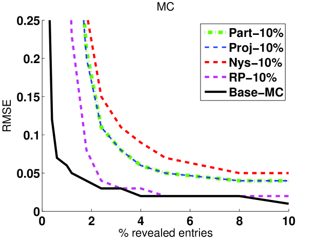
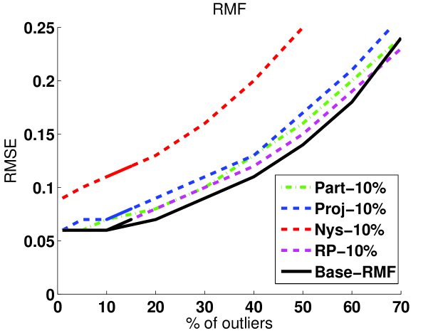
(a)	(b)
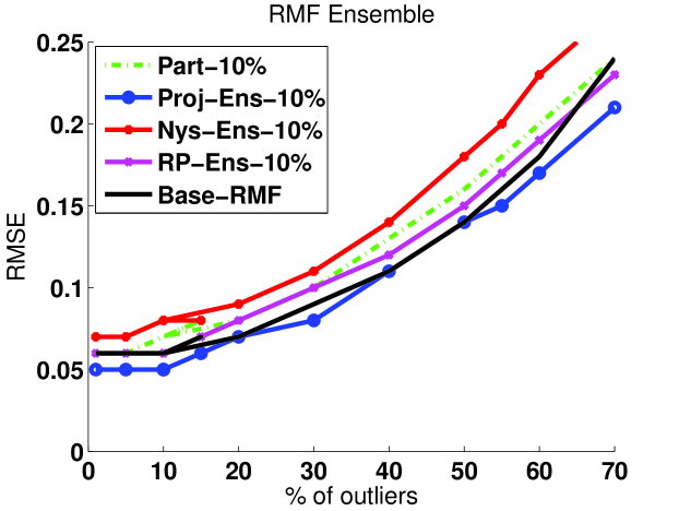
(c)	(d)

Figure 1: Recovery error of DFC relative to base algorithms.

We first explored the estimation error of DFC as a function of $s$, using ($m=10$K, $r=10)$ with varying observation sparsity for MC and ($m=1$K, $r=10)$ with a varying percentage of outliers for RMF. The results are summarized in Figure 1. In both MC and RMF, the gaps in estimation between APG and DFC are small when sampling only 10% of rows and columns. Moreover, of the standard DFC algorithms, DFC-RP performs the best, as shown in Figures 1(a) and (b). Ensembling improves the performance of DFC-Nys and DFC-Proj, as shown in Figures 1(c) and (d), and DFC-Proj-Ens in particular consistently outperforms Partition and DFC-Nys-Ens, slightly outperforms DFC-RP, and matches the performance of APG for most settings of $s$. In practice we observe that ${\mathbf{L}}^{rp}$ equals the optimal (with respect to the spectral or Frobenius norm) rank-$k$ approximation of $[\hat{\mathbf{C}}_{1},\ldots,\hat{\mathbf{C}}_{t}]$, and thus the performance of DFC-RP consistently matches that of DFC-RP-Ens. We therefore omit the DFC-RP-Ens results in the remainder this section.

We next explored the speed-up of DFC as a function of matrix size. For MC, we revealed $4\%$ of the matrix entries and set $r=0.001\cdot m$, while for RMF we fixed the percentage of outliers to $10\%$ and set $r=0.01\cdot m$. We sampled $10\%$ of rows and columns and observed that estimation errors were comparable to the errors presented in Figure 1 for similar settings of $s$; in particular, at all values of $n$ for both MC and RMF, the errors of APG and DFC-Proj-Ens were nearly identical. Our timing results, presented in Figure 2, illustrate a near-linear speed-up for MC and a superlinear speed-up for RMF across varying matrix sizes. Note that the timing curves of the DFC algorithms and Partition all overlap, a fact that highlights the minimal computational cost of the final matrix approximation step.

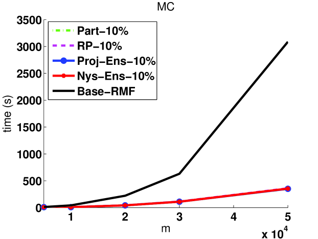
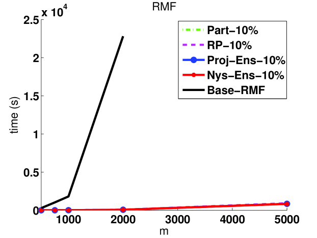
Figure 2: Speed-up of DFC relative to base algorithms.

6.2 Collaborative Filtering

Collaborative filtering for recommender systems is one prevalent real-world application of noisy matrix completion. A collaborative filtering dataset can be interpreted as the incomplete observation of a ratings matrix with columns corresponding to users and rows corresponding to items. The goal is to infer the unobserved entries of this ratings matrix. We evaluate DFC on two of the largest publicly available collaborative filtering datasets: MovieLens 10M ($m=4$K, $n=6$K, $s>10$M) and the Netflix Prize dataset ($m=18$K, $n=480$K, $s>100$M). To generate test sets drawn from the training distribution, for each dataset, we aggregated all available rating data into a single training set and withheld test entries uniformly at random, while ensuring that at least one training observation remained in each row and column. The algorithms were then run on the remaining training portions and evaluated on the test portions of each split. The results, averaged over three train-test splits, are summarized in Table 1. Notably, DFC-Proj, DFC-Proj-Ens, DFC-Nys-Ens, and DFC-RP all outperform Partition, and DFC-Proj-Ens performs comparably to APG while providing a nearly linear parallel time speed-up. Similar to the simulation results presented in Figure 1, DFC-RP performs the best of the standard DFC algorithms, though DFC-Proj-Ens slightly outperforms DFC-RP. Moreover, the poorer performance of DFC-Nys can be in part explained by the asymmetry of these problems. Since these matrices have many more columns than rows, MF on column submatrices is inherently easier than MF on row submatrices, and for DFC-Nys, we observe that $\hat{\mathbf{C}}$ is an accurate estimate while $\hat{\mathbf{R}}$ is not.

Table 1: Performance of DFC relative to base algorithm APG on collaborative filtering tasks.

Method	MovieLens 10M		Netflix
	RMSE	Time	RMSE	Time
Base algorithm (APG)	0.8005	552.3s	0.8433	4775.4s
Partition-25%	0.8146	146.2s	0.8451	1274.6s
Partition-10%	0.8461	56.0s	0.8491	548.0s
DFC-Nys-25%	0.8449	141.9s	0.8832	1541.2s
DFC-Nys-10%	0.8776	82.5s	0.9228	797.4s
DFC-Nys-Ens-25%	0.8085	153.5s	0.8486	1661.2s
DFC-Nys-Ens-10%	0.8328	96.2s	0.8613	909.8s
DFC-Proj-25%	0.8061	146.3s	0.8436	1274.8s
DFC-Proj-10%	0.8270	56.0s	0.8486	548.1s
DFC-Proj-Ens-25%	0.7944	146.3s	0.8411	1274.8s
DFC-Proj-Ens-10%	0.8117	56.0s	0.8434	548.1s
DFC-RP-25%	0.8027	147.4s	0.8438	1283.6s
DFC-RP-10%	0.8074	56.2s	0.8448	550.1s

6.3 Background Modeling in Computer Vision

Background modeling has important practical ramifications for detecting activity in surveillance video. This problem can be framed as an application of noisy RMF, where each video frame is a column of some matrix (${\mathbf{M}})$, the background model is low-rank (${\mathbf{L}}_{0})$, and moving objects and background variations, e.g., changes in illumination, are outliers (${\mathbf{S}}_{0})$. We evaluate DFC on two videos: ‘Hall’ ($200$ frames of size $176\times 144)$ contains significant foreground variation and was studied by Candès et al. [2], while ‘Lobby’ ($1546$ frames of size $168\times 120)$ includes many changes in illumination (a smaller video with $250$ frames was studied by Candès et al. [2]). We focused on DFC-Proj-Ens, due to its superior performance in previous experiments, and measured the RMSE between the background model estimated by DFC and that of APG. On both videos, DFC-Proj-Ens estimated nearly the same background model as the full APG algorithm in a small fraction of the time. On ‘Hall,’ the DFC-Proj-Ens-5% and DFC-Proj-Ens-0.5% models exhibited RMSEs of $0.564$ and $1.55$, quite small given pixels with $256$ intensity values. The associated running time was reduced from $342.5$s for APG to real-time ($5.2$s for a $13$s video) for DFC-Proj-Ens-0.5%. Snapshots of the results are presented in Figure 3. On ‘Lobby,’ the RMSE of DFC-Proj-Ens-4% was $0.64$, and the speed-up over APG was more than 20X, i.e., the running time reduced from $16557$s to $792$s.

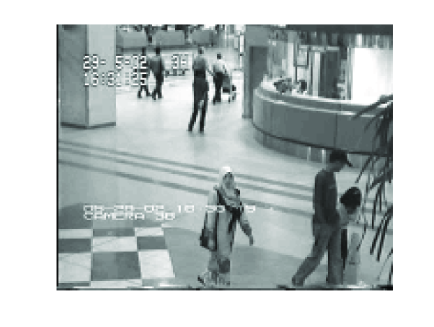
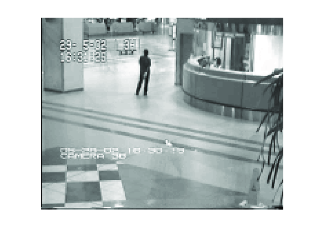
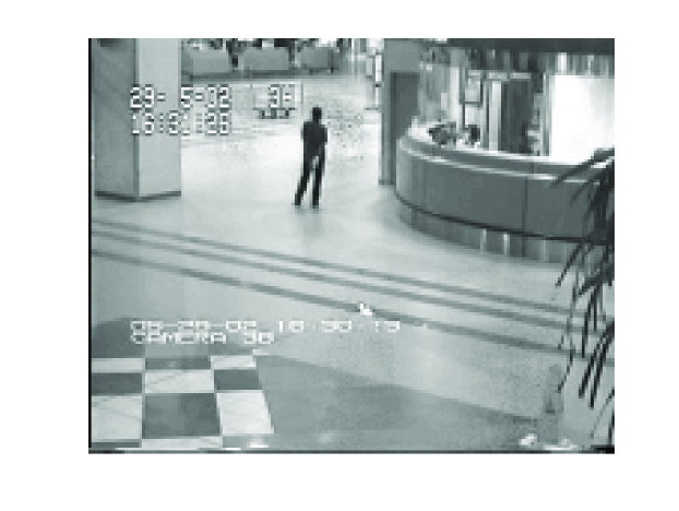
Original frame	APG	5% sampled	0.5% sampled
	(342.5s)	(24.2s)	(5.2s)

Figure 3: Sample ‘Hall’ estimation by APG, DFC-Proj-Ens-5%, and DFC-Proj-Ens-.5%.

7 Conclusions

To improve the scalability of existing matrix factorization algorithms while leveraging the ubiquity of parallel computing architectures, we introduced, evaluated, and analyzed DFC, a divide-and-conquer framework for noisy matrix factorization with missing entries or outliers. DFC is trivially parallelized and particularly well suited for distributed environments given its low communication footprint. Moreover, DFC provably maintains the estimation guarantees of its base algorithm, even in the presence of noise, and yields linear to super-linear speedups in practice.

A number of natural follow-up questions suggest themselves. First, can the sampling complexities and conclusions of our theoretical analyses be strengthened? For example, can the $(2+\epsilon)$ approximation guarantees of our master theorems be sharpened to $(1+\epsilon)$? Second, how does DFC perform when paired with alternative base algorithms, having no theoretical guarantees but displaying other practical benefits? These open questions are fertile ground for future work.

Appendix A Proof of Theorem 5: Subsampled Regression under Incoherence

We now give a proof of Thm. 5. While the results of this section are stated in terms of i.i.d. with-replacement sampling of columns and rows, a concise argument due to Hoeffding [16, Sec. 6] implies the same conclusions when columns and rows are sampled without replacement.

Our proof of Thm. 5 will require a strengthened version of the randomized $\ell_{2}$ regression work of Drineas et al. [9, Thm. 5]. The proof of Thm. 5 of Drineas et al. [9] relies heavily on the fact that ${\|{{\mathbf{A}}{\mathbf{B}}-{\mathbf{G}}{\mathbf{H}}}\|}_{F}\leq\frac{\epsilon}{2}{\|{{\mathbf{A}}}\|}_{F}{\|{{\mathbf{B}}}\|}_{F}$ with probability at least 0.9, when ${\mathbf{G}}$ and ${\mathbf{H}}$ contain sufficiently many rescaled columns and rows of ${\mathbf{A}}$ and ${\mathbf{B}}$, sampled according to a particular non-uniform probability distribution. A result of Hsu et al. [19], modified to allow for slack in the probabilities, establishes a related claim with improved sampling complexity.

Lemma 20 ([19, Example 4.3]).

Given a matrix ${\mathbf{A}}\in\mathbb{R}^{m\times k}$ with $r\geq\mathrm{rank}({{\mathbf{A}}})$, an error tolerance $\epsilon\in(0,1]$, and a failure probability $\delta\in(0,1]$, define probabilities $p_{j}$ satisfying

$$p_{j} \geq\frac{\beta}{Z}{\|{{\mathbf{A}}_{(j)}}\|}^{2},\quad Z=\sum_{j}{\|{{\mathbf{A}}_{(j)}}\|}^{2},\quad\text{and}\quad{\textstyle\sum}_{j=1}^{k}p_{j}=1$$ (7)

for some $\beta\in(0,1]$. Let ${\mathbf{G}}\in\mathbb{R}^{m\times l}$ be a column submatrix of ${\mathbf{A}}$ in which exactly $l\geq 48r\log(4r/(\beta\delta))/(\beta\epsilon^{2})$ columns are selected in i.i.d. trials in which the $j$-th column is chosen with probability $p_{j}$. Further, let ${\mathbf{D}}\in\mathbb{R}^{l\times l}$ be a diagonal rescaling matrix with entry ${\mathbf{D}}_{tt}=1/\sqrt{lp_{j}}$ whenever the $j$-th column of ${\mathbf{A}}$ is selected on the $t$-th sampling trial, for $t=1,\ldots,l$. Then, with probability at least $1-\delta$,

$${\|{{\mathbf{A}}{\mathbf{A}}^{\top}-{\mathbf{G}}{\mathbf{D}}{\mathbf{D}}{\mathbf{G}}^{\top}}\|}_{2}\leq\frac{\epsilon}{2}{\|{{\mathbf{A}}}\|}_{2}^{2}.$$

Using Lem. 20, we now establish a stronger version of Lem. 1 of Drineas et al. [9]. For a given $\beta\in(0,1]$ and ${\mathbf{L}}\in\mathbb{R}^{m\times n}$ with rank $r$, we first define column sampling probabilities $p_{j}$ satisfying

$$p_{j} \geq\frac{\beta}{r}{\|{({\mathbf{V}}_{L})_{(j)}}\|}^{2}\quad\text{and}\quad{\textstyle\sum}_{j=1}^{n}p_{j}=1.$$ (8)

We further let ${\mathbf{S}}\in\mathbb{R}^{n\times l}$ be a random binary matrix with independent columns, where a single 1 appears in each column, and ${\mathbf{S}}_{jt}=1$ with probability $p_{j}$ for each $t\in\{1,\ldots,l\}$. Moreover, let ${\mathbf{D}}\in\mathbb{R}^{l\times l}$ be a diagonal rescaling matrix with entry ${\mathbf{D}}_{tt}=1/\sqrt{lp_{j}}$ whenever ${\mathbf{S}}_{jt}=1$. Postmultiplication by ${\mathbf{S}}$ is equivalent to selecting $l$ random columns of a matrix, independently and with replacement. Under this notation, we establish the following lemma:

Lemma 21.

Let $\epsilon\in(0,1],$ and define ${\mathbf{V}}_{l}^{\top}={\mathbf{V}}_{L}^{\top}{\mathbf{S}}$ and $\Gamma=({\mathbf{V}}_{l}^{\top}{\mathbf{D}})^{+}-({\mathbf{V}}_{l}^{\top}{\mathbf{D}})^{\top}$. If $l\geq 48r\log(4r/(\beta\delta))/(\beta\epsilon^{2})$ for $\delta\in(0,1]$ then with probability at least $1-\delta$:

$$\mathrm{rank}({{\mathbf{V}}_{l}})=\mathrm{rank}({{\mathbf{V}}_{L}})=\mathrm{rank}({{\mathbf{L}}})$$

$${\|{\Gamma}\|}_{2}={\|{{\mathbf{\Sigma}}_{V_{l}^{\top}D}^{-1}-{\mathbf{\Sigma}}_{V_{l}^{\top}D}}\|}_{2}$$

$$({\mathbf{L}}{\mathbf{S}}{\mathbf{D}})^{+}=({\mathbf{V}}_{l}^{\top}{\mathbf{D}})^{+}{\mathbf{\Sigma}}_{L}^{-1}{\mathbf{U}}_{L}^{\top}$$

$${\|{{\mathbf{\Sigma}}_{V_{l}^{\top}D}^{-1}-{\mathbf{\Sigma}}_{V_{l}^{\top}D}}\|}_{2}\leq\epsilon/\sqrt{2}.$$

Proof    By Lem. 20, for all $1\leq i\leq r$,

$$|1-\sigma_{i}^{2}({\mathbf{V}}_{l}^{\top}{\mathbf{D}})| =|\sigma_{i}({\mathbf{V}}_{L}^{\top}{\mathbf{V}}_{L})-\sigma_{i}({\mathbf{V}}_{l}^{\top}{\mathbf{D}}{\mathbf{D}}{\mathbf{V}}_{l})|$$

$$\leq{\|{{\mathbf{V}}_{L}^{\top}{\mathbf{V}}_{L}-{\mathbf{V}}_{L}^{\top}{\mathbf{S}}{\mathbf{D}}{\mathbf{D}}{\mathbf{S}}^{\top}{\mathbf{V}}_{L}}\|}_{2}$$

$$\leq\epsilon/2{\|{{\mathbf{V}}_{L}^{\top}}\|}_{2}^{2}=\epsilon/2,$$

where $\sigma_{i}(\cdot)$ is the $i$-th largest singular value of a given matrix. Since $\epsilon/2\leq 1/2$, each singular value of ${\mathbf{V}}_{l}$ is positive, and so $\mathrm{rank}({{\mathbf{V}}_{l}})=\mathrm{rank}({{\mathbf{V}}_{L}})=\mathrm{rank}({{\mathbf{L}}})$. The remainder of the proof is identical to that of Lem. 1 of Drineas et al. [9]. ∎

Lem. 21 immediately yields improved sampling complexity for the randomized $\ell_{2}$ regression of Drineas et al. [9]:

Proposition 22.

Suppose ${\mathbf{B}}\in\mathbb{R}^{p\times n}$ and $\epsilon\in(0,1]$. If $l\geq 3200r\log(4r/(\beta\delta))/(\beta\epsilon^{2})$ for $\delta\in(0,1]$, then with probability at least $1-\delta-0.2$:

$${\|{{\mathbf{B}}-{\mathbf{B}}{\mathbf{S}}{\mathbf{D}}({\mathbf{L}}{\mathbf{S}}{\mathbf{D}})^{+}{\mathbf{L}}}\|}_{F}\leq(1+\epsilon){\|{{\mathbf{B}}-{\mathbf{B}}{\mathbf{L}}^{+}{\mathbf{L}}}\|}_{F}.$$

Proof    The proof is identical to that of Thm. 5 of Drineas et al. [9] once Lem. 21 is substituted for Lem. 1 of Drineas et al. [9]. ∎

A typical application of Prop. 22 would involve performing a truncated SVD of ${\mathbf{M}}$ to obtain the statistical leverage scores, ${\|{({\mathbf{V}}_{L})_{(j)}}\|}^{2}$, used to compute the column sampling probabilities of Eq. (8). Here, we will take advantage of the slack term, $\beta$, allowed in the sampling probabilities of Eq. (8) to show that uniform column sampling gives rise to the same estimation guarantees for column projection approximations when ${\mathbf{L}}$ is sufficiently incoherent.

To prove Thm. 5, we first notice that $n\geq r\mu_{0}({\mathbf{V}}_{L})$ and hence

$$l \geq 3200r\mu_{0}({\mathbf{V}}_{L})\log(4r\mu_{0}({\mathbf{V}}_{L})/\delta)/\epsilon^{2}$$

$$\geq 3200r\log(4r/(\beta\delta))/(\beta\epsilon^{2})$$

whenever $\beta\geq 1/\mu_{0}({\mathbf{V}}_{L})$. Thus, we may apply Prop. 22 with $\beta=1/\mu_{0}({\mathbf{V}}_{L})\in(0,1]$ and $p_{j}=1/n$ by noting that

$$\frac{\beta}{r}{\|{({\mathbf{V}}_{L})_{(j)}}\|}^{2}\leq\frac{\beta}{r}\frac{r}{n}\mu_{0}({\mathbf{V}}_{L})=\frac{1}{n}=p_{j}$$

for all $j$, by the definition of $\mu_{0}({\mathbf{V}}_{L})$. By our choice of probabilities, ${\mathbf{D}}={\mathbf{I}}\sqrt{n/l}$, and hence

$${\|{{\mathbf{B}}-{\mathbf{B}}_{C}{\mathbf{L}}_{C}^{+}{\mathbf{L}}}\|}_{F}={\|{{\mathbf{B}}-{\mathbf{B}}_{C}{\mathbf{D}}({\mathbf{L}}_{C}{\mathbf{D}})^{+}{\mathbf{L}}}\|}_{F}\leq(1+\epsilon){\|{{\mathbf{B}}-{\mathbf{B}}{\mathbf{L}}^{+}{\mathbf{L}}}\|}_{F}$$

with probability at least $1-\delta-0.2$, as desired.

Appendix B Proof of Lemma 4: Conservation of Incoherence

Since for all $n>1$,

$$c\log(n)\log(1/\delta)=({c}/{4})\log(n^{4})\log(1/\delta)\geq 48\log(4n^{2}/\delta)\geq 48\log(4r\mu_{0}({\mathbf{V}}_{L})/(\delta/n))$$

as $n\geq r\mu_{0}({\mathbf{V}}_{L})$, claim $i$ follows immediately from Lemma 21 with $\beta=1/\mu_{0}({\mathbf{V}}_{L})$, $p_{j}=1/n$ for all $j$, and ${\mathbf{D}}={\mathbf{I}}\sqrt{n/l}$. When $\mathrm{rank}({{\mathbf{L}}_{C}})=\mathrm{rank}({{\mathbf{L}}})$, Lemma 1 of Mohri and Talwalkar [32] implies that ${\mathbf{P}}_{U_{L_{C}}}={\mathbf{P}}_{U_{L}}$, which in turn implies claim $ii$.

To prove claim $iii$ given the conclusions of Lemma 21, assume, without loss of generality, that ${\mathbf{V}}_{l}$ consists of the first $l$ rows of ${\mathbf{V}}_{L}$. Then if ${\mathbf{L}}_{C}={\mathbf{U}}_{L}{\mathbf{\Sigma}}_{L}{\mathbf{V}}_{l}^{\top}$ has $\mathrm{rank}({{\mathbf{L}}_{C}})=\mathrm{rank}({{\mathbf{L}}})=r$, the matrix ${\mathbf{V}}_{l}$ must have full column rank. Thus we can write

$${\mathbf{L}}_{C}^{+}{\mathbf{L}}_{C} =({\mathbf{U}}_{L}{\mathbf{\Sigma}}_{L}{\mathbf{V}}_{l}^{\top})^{+}{\mathbf{U}}_{L}{\mathbf{\Sigma}}_{L}{\mathbf{V}}_{l}^{\top}$$

$$=({\mathbf{\Sigma}}_{L}{\mathbf{V}}_{l}^{\top})^{+}{\mathbf{U}}_{L}^{+}{\mathbf{U}}_{L}{\mathbf{\Sigma}}_{L}{\mathbf{V}}_{l}^{\top}$$

$$=({\mathbf{\Sigma}}_{L}{\mathbf{V}}_{l}^{\top})^{+}{\mathbf{\Sigma}}_{L}{\mathbf{V}}_{l}^{\top}$$

$$=({\mathbf{V}}_{l}^{\top})^{+}{\mathbf{\Sigma}}_{L}^{+}{\mathbf{\Sigma}}_{L}{\mathbf{V}}_{l}^{\top}$$

$$=({\mathbf{V}}_{l}^{\top})^{+}{\mathbf{V}}_{l}^{\top}$$

$$={\mathbf{V}}_{l}({\mathbf{V}}_{l}^{\top}{\mathbf{V}}_{l})^{-1}{\mathbf{V}}_{l}^{\top},$$

where the second and third equalities follow from ${\mathbf{U}}_{L}$ having orthonormal columns, the fourth and fifth result from ${\mathbf{\Sigma}}_{L}$ having full rank and ${\mathbf{V}}_{l}$ having full column rank, and the sixth follows from ${\mathbf{V}}_{l}^{\top}$ having full row rank.

Now, denote the right singular vectors of ${\mathbf{L}}_{C}$ by ${\mathbf{V}}_{L_{C}}\in\mathbb{R}^{l\times r}$. Observe that ${\mathbf{P}}_{V_{L_{C}}}={\mathbf{V}}_{L_{C}}{\mathbf{V}}_{L_{C}}^{\top}={\mathbf{L}}_{C}^{+}{\mathbf{L}}_{C}$, and define ${\mathbf{e}}_{i,l}$ as the $i$th column of ${\mathbf{I}}_{l}$ and ${\mathbf{e}}_{i,n}$ as the $i$th column of ${\mathbf{I}}_{n}$. Then we have,

$$\mu_{0}({\mathbf{V}}_{L_{C}}) =\frac{l}{r}\max_{1\leq i\leq l}{\|{{\mathbf{P}}_{V_{L_{C}}}{\mathbf{e}}_{i,l}}\|}^{2}$$

$$=\frac{l}{r}\max_{1\leq i\leq l}{\mathbf{e}}_{i,l}^{\top}{\mathbf{L}}_{C}^{+}{\mathbf{L}}_{C}{\mathbf{e}}_{i,l}$$

$$=\frac{l}{r}\max_{1\leq i\leq l}{\mathbf{e}}_{i,l}^{\top}({\mathbf{V}}_{l}^{\top})^{+}{\mathbf{V}}_{l}^{\top}{\mathbf{e}}_{i,l}$$

$$=\frac{l}{r}\max_{1\leq i\leq l}{\mathbf{e}}_{i,l}^{\top}{\mathbf{V}}_{l}({\mathbf{V}}_{l}^{\top}{\mathbf{V}}_{l})^{-1}{\mathbf{V}}_{l}^{\top}{\mathbf{e}}_{i,l}$$

$$=\frac{l}{r}\max_{1\leq i\leq l}{\mathbf{e}}_{i,n}^{\top}{\mathbf{V}}_{L}({\mathbf{V}}_{l}^{\top}{\mathbf{V}}_{l})^{-1}{\mathbf{V}}_{L}^{\top}{\mathbf{e}}_{i,n},$$

where the final equality follows from ${\mathbf{V}}_{l}^{\top}{\mathbf{e}}_{i,l}={\mathbf{V}}_{L}^{\top}{\mathbf{e}}_{i,n}$ for all $1\leq i\leq l$.

Now, defining ${\mathbf{Q}}={\mathbf{V}}_{l}^{\top}{\mathbf{V}}_{l}$ we have

$$\mu_{0}({\mathbf{V}}_{L_{C}}) =\frac{l}{r}\max_{1\leq i\leq l}{\mathbf{e}}_{i,n}^{\top}{\mathbf{V}}_{L}{\mathbf{Q}}^{-1}{\mathbf{V}}_{L}^{\top}{\mathbf{e}}_{i,n}$$

$$=\frac{l}{r}\max_{1\leq i\leq l}\operatorname{Tr}\mathopen{}\mathclose{{}\left[{{\mathbf{e}}_{i,n}^{\top}{\mathbf{V}}_{L}{\mathbf{Q}}^{-1}{\mathbf{V}}_{L}^{\top}{\mathbf{e}}_{i,n}}}\right]$$

$$=\frac{l}{r}\max_{1\leq i\leq l}\operatorname{Tr}\mathopen{}\mathclose{{}\left[{{\mathbf{Q}}^{-1}{\mathbf{V}}_{L}^{\top}{\mathbf{e}}_{i,n}{\mathbf{e}}_{i,n}^{\top}{\mathbf{V}}_{L}}}\right]$$

$$\leq\frac{l}{r}{\|{{\mathbf{Q}}^{-1}}\|}_{2}\max_{1\leq i\leq l}{\|{{\mathbf{V}}_{L}^{\top}{\mathbf{e}}_{i,n}{\mathbf{e}}_{i,n}^{\top}{\mathbf{V}}_{L}}\|}_{*}\ ,$$

by Hölder’s inequality for Schatten $p$-norms. Since ${\mathbf{V}}_{L}^{\top}{\mathbf{e}}_{i,n}{\mathbf{e}}_{i,n}^{\top}{\mathbf{V}}_{L}$ has rank one, we can explicitly compute its trace norm as ${\|{{\mathbf{V}}_{L}^{\top}{\mathbf{e}}_{i,n}}\|}^{2}={\|{{\mathbf{P}}_{V_{L}}{\mathbf{e}}_{i,n}}\|}^{2}$. Hence,

$$\mu_{0}({\mathbf{V}}_{L_{C}}) \leq\frac{l}{r}{\|{{\mathbf{Q}}^{-1}}\|}_{2}\max_{1\leq i\leq l}{\|{{\mathbf{P}}_{V_{L}}{\mathbf{e}}_{i,n}}\|}^{2}$$

$$\leq\frac{l}{r}\frac{r}{n}{\|{{\mathbf{Q}}^{-1}}\|}_{2}\bigg{(}\frac{n}{r}\max_{1\leq i\leq n}{\|{{\mathbf{P}}_{V_{L}}{\mathbf{e}}_{i,n}}\|}^{2}\bigg{)}$$

$$=\frac{l}{n}{\|{{\mathbf{Q}}^{-1}}\|}_{2}\mu_{0}({\mathbf{V}}_{L})\,,$$

by the definition of $\mu_{0}$-coherence. The proof of Lemma 21 established that the smallest singular value of $\frac{n}{l}{\mathbf{Q}}={\mathbf{V}}_{l}^{\top}{\mathbf{D}}{\mathbf{D}}{\mathbf{V}}_{l}$ is lower bounded by $1-\frac{\epsilon}{2}$ and hence ${\|{{\mathbf{Q}}^{-1}}\|}_{2}\leq\frac{n}{l(1-\epsilon/2)}$. Thus, we conclude that $\mu_{0}({\mathbf{V}}_{L_{C}})\leq\mu_{0}({\mathbf{V}}_{L})/(1-\epsilon/2)$.

To prove claim $iv$ under Lemma 21, we note that

$$\mu_{1}({\mathbf{L}}_{C}) =\sqrt{\frac{ml}{r}}\max_{\begin{subarray}{c}1\leq i\leq m\\ 1\leq j\leq l\end{subarray}}|{\mathbf{e}}_{i,m}^{\top}{\mathbf{U}}_{L_{C}}{\mathbf{V}}_{L_{C}}^{\top}{\mathbf{e}}_{j,l}|$$

$$\leq\sqrt{\frac{ml}{r}}\max_{1\leq i\leq m}{\|{{\mathbf{U}}_{L_{C}}^{\top}{\mathbf{e}}_{i,m}}\|}\max_{1\leq j\leq l}{\|{{\mathbf{V}}_{L_{C}}^{\top}{\mathbf{e}}_{j,l}}\|}$$

$$=\sqrt{r}\bigg{(}\sqrt{\frac{m}{r}}\max_{1\leq i\leq m}{\|{{\mathbf{P}}_{U_{L_{C}}}{\mathbf{e}}_{i,m}}\|}\bigg{)}\bigg{(}\sqrt{\frac{l}{r}}\max_{1\leq j\leq l}{\|{{\mathbf{P}}_{V_{L_{C}}}{\mathbf{e}}_{j,l}}\|}\bigg{)}$$

$$=\sqrt{r\mu_{0}({\mathbf{U}}_{L_{C}})\mu_{0}({\mathbf{V}}_{L_{C}})}\leq\sqrt{r\mu_{0}({\mathbf{U}}_{L})\mu_{0}({\mathbf{V}}_{L})/(1-\epsilon/2)}$$

by Hölder’s inequality for Schatten $p$-norms, the definition of $\mu_{0}$-coherence, and claims $ii$ and $iii$.

Appendix C Proof of Corollary 6: Column Projection under Incoherence

Fix $c=48000/\log(1/0.45)$, and notice that for $n>1$,

$$48000\log(n)\geq 3200\log(n^{5})\geq 3200\log(16n).$$

Hence $l\geq 3200r\mu_{0}({\mathbf{V}}_{L})\log(16n)(\log(\delta)/\log(0.45))/\epsilon^{2}.$

Now partition the columns of ${\mathbf{C}}$ into $b=\log(\delta)/\log(0.45)$ submatrices, ${\mathbf{C}}=[{\mathbf{C}}_{1},\cdots,{\mathbf{C}}_{b}]$, each with $a=l/b$ columns, and let $[{\mathbf{L}}_{C_{1}},\cdots,{\mathbf{L}}_{C_{b}}]$ be the corresponding partition of ${\mathbf{L}}_{C}$. Since

$$a\geq 3200r\mu_{0}({\mathbf{V}}_{L})\log(4n/0.25)/\epsilon^{2},$$

we may apply Prop. 22 independently for each $i$ to yield

$${\|{{\mathbf{M}}-{\mathbf{C}}_{i}{\mathbf{L}}_{C_{i}}^{+}{\mathbf{L}}}\|}_{F}\leq(1+\epsilon){\|{{\mathbf{M}}-{\mathbf{M}}{\mathbf{L}}^{+}{\mathbf{L}}}\|}_{F}\leq(1+\epsilon){\|{{\mathbf{M}}-{\mathbf{L}}}\|}_{F}$$ (9)

with probability at least $0.55$, since ${\mathbf{M}}{\mathbf{L}}^{+}$ minimizes ${\|{{\mathbf{M}}-{\mathbf{Y}}{\mathbf{L}}}\|}_{F}$ over all ${\mathbf{Y}}\in\mathbb{R}^{m\times m}$.

Since each ${\mathbf{C}}_{i}={\mathbf{C}}{\mathbf{S}}_{i}$ for some matrix ${\mathbf{S}}_{i}$ and ${\mathbf{C}}^{+}{\mathbf{M}}$ minimizes ${\|{{\mathbf{M}}-{\mathbf{C}}{\mathbf{X}}}\|}_{F}$ over all ${\mathbf{X}}\in\mathbb{R}^{l\times n}$, it follows that

$${\|{{\mathbf{M}}-{\mathbf{C}}{\mathbf{C}}^{+}{\mathbf{M}}}\|}_{F}\leq{\|{{\mathbf{M}}-{\mathbf{C}}_{i}{\mathbf{L}}_{C_{i}}^{+}{\mathbf{L}}}\|}_{F},$$

for each $i$. Hence, if

$${\|{{\mathbf{M}}-{\mathbf{C}}{\mathbf{C}}^{+}{\mathbf{M}}}\|}_{F}\leq(1+\epsilon){\|{{\mathbf{M}}-{\mathbf{L}}}\|}_{F},$$

fails to hold, then, for each $i$, Eq. (9) also fails to hold. The desired conclusion therefore must hold with probability at least $1-0.45^{b}=1-\delta$.

Appendix D Proof of Corollary 7: Generalized Nyström Method under Incoherence

With $c=48000/\log(1/0.45)$ as in Cor. 6, we notice that for $m>1$,

$$48000\log(m)=16000\log(m^{3})\geq 16000\log(4m).$$

Therefore,

$$d \geq 16000r\mu_{0}({\mathbf{U}}_{C})\log(4m)(\log(\delta^{\prime})/\log(0.45))/\epsilon^{2}$$

$$\geq 3200r\mu_{0}({\mathbf{U}}_{C})\log(4m/\delta^{\prime})/\epsilon^{2},$$

for all $m>1$ and $\delta^{\prime}\leq 0.8$. Hence, we may apply Thm. 5 and Cor. 6 in turn to obtain

$${\|{{\mathbf{M}}-{\mathbf{C}}{\mathbf{W}}^{+}{\mathbf{R}}}\|}_{F}\leq(1+\epsilon){\|{{\mathbf{M}}-{\mathbf{C}}{\mathbf{C}}^{+}{\mathbf{M}}}\|}_{F}\leq(1+\epsilon)^{2}{\|{{\mathbf{M}}-{\mathbf{L}}}\|}$$

with probability at least $(1-\delta)(1-\delta^{\prime}-0.2)$ by independence.

Appendix E Proof of Corollary 8: Noiseless Generalized Nyström Method under Incoherence

Since $\mathrm{rank}({{\mathbf{L}}})=r$, ${\mathbf{L}}$ admits a decomposition ${\mathbf{L}}={\mathbf{Y}}^{\top}{\mathbf{Z}}$ for some matrices ${\mathbf{Y}}\in\mathbb{R}^{r\times m}$ and ${\mathbf{Z}}\in\mathbb{R}^{r\times n}$. In particular, let ${\mathbf{Y}}^{\top}={\mathbf{U}}_{L}{\mathbf{\Sigma}}_{L}^{\frac{1}{2}}$ and ${\mathbf{Z}}={\mathbf{\Sigma}}_{L}^{\frac{1}{2}}{\mathbf{V}}_{L}^{\top}$. By block partitioning ${\mathbf{Y}}$ and ${\mathbf{Z}}$ as ${\mathbf{Y}}=\begin{bmatrix}{\mathbf{Y}}_{1}&{\mathbf{Y}}_{2}\end{bmatrix}$ and ${\mathbf{Z}}=\begin{bmatrix}{\mathbf{Z}}_{1}&{\mathbf{Z}}_{2}\end{bmatrix}$ for ${\mathbf{Y}}_{1}\in\mathbb{R}^{r\times d}$ and ${\mathbf{Z}}_{1}\in\mathbb{R}^{r\times l}$, we may write ${\mathbf{W}}={\mathbf{Y}}_{1}^{\top}{\mathbf{Z}}_{1},{\mathbf{C}}={\mathbf{Y}}^{\top}{\mathbf{Z}}_{1},$ and ${\mathbf{R}}={\mathbf{Y}}_{1}^{\top}{\mathbf{Z}}$. Note that we assume that the generalized Nyström approximation is generated from sampling the first $l$ columns and the first $d$ rows of ${\mathbf{L}}$, which we do without loss of generality since the rows and columns of the original low-rank matrix can always be permutated to match this assumption.

Prop. 23 shows that, like the Nyström method [23], the generalized Nyström method yields exact recovery of ${\mathbf{L}}$ whenever $\mathrm{rank}({{\mathbf{L}}})=\mathrm{rank}({{\mathbf{W}}})$. The same result was established in Wang et al. [44] with a different proof.

Proposition 23.

Suppose $r=\mathrm{rank}({{\mathbf{L}}})\leq\min(d,l)$ and $\mathrm{rank}({{\mathbf{W}}})=r$. Then ${\mathbf{L}}={\mathbf{L}}^{nys}$.

Proof    By appealing to our factorized block decomposition, we may rewrite the generalized Nyström approximation as ${\mathbf{L}}^{nys}={\mathbf{C}}{\mathbf{W}}^{+}{\mathbf{R}}={\mathbf{Y}}^{\top}{\mathbf{Z}}_{1}({\mathbf{Y}}_{1}^{\top}{\mathbf{Z}}_{1})^{+}{\mathbf{Y}}_{1}^{\top}{\mathbf{Z}}$. We first note that $\mathrm{rank}({{\mathbf{W}}})=r$ implies that $\mathrm{rank}({{\mathbf{Y}}_{1}})=r$ and $\mathrm{rank}({{\mathbf{Z}}_{1}})=r$ so that ${\mathbf{Z}}_{1}{\mathbf{Z}}_{1}^{\top}$ and ${\mathbf{Y}}_{1}{\mathbf{Y}}_{1}^{\top}$ are full-rank. Hence, $({\mathbf{Y}}_{1}^{\top}{\mathbf{Z}}_{1})^{+}={\mathbf{Z}}_{1}^{\top}({\mathbf{Z}}_{1}{\mathbf{Z}}_{1}^{\top})^{-1}({\mathbf{Y}}_{1}{\mathbf{Y}}_{1}^{\top})^{-1}{\mathbf{Y}}_{1},$ yielding

$${\mathbf{L}}^{nys}={\mathbf{Y}}^{\top}{\mathbf{Z}}_{1}{\mathbf{Z}}_{1}^{\top}({\mathbf{Z}}_{1}{\mathbf{Z}}_{1}^{\top})^{-1}({\mathbf{Y}}_{1}{\mathbf{Y}}_{1}^{\top})^{-1}{\mathbf{Y}}_{1}{\mathbf{Y}}_{1}^{\top}{\mathbf{Z}}={\mathbf{Y}}^{\top}{\mathbf{Z}}={\mathbf{L}}.$$

∎

Prop. 23 allows us to lower bound the probability of exact recovery with the probability of randomly selecting a rank-$r$ submatrix. As $\mathrm{rank}({{\mathbf{W}}})=r$ iff both $\mathrm{rank}({{\mathbf{Y}}_{1}})=r$ and $\mathrm{rank}({{\mathbf{Z}}_{1}})=r$, it suffices to characterize the probability of selecting full rank submatrices of ${\mathbf{Y}}$ and ${\mathbf{Z}}$. Following the treatment of the Nyström method in Talwalkar and Rostamizadeh [41], we note that ${\mathbf{\Sigma}}_{L}^{-\frac{1}{2}}{\mathbf{Z}}={\mathbf{V}}_{L}^{\top}$ and hence that ${\mathbf{Z}}_{1}^{\top}{\mathbf{\Sigma}}_{{\mathbf{L}}}^{-\frac{1}{2}}={\mathbf{V}}_{l}$ where ${\mathbf{V}}_{l}\in\mathbb{R}^{l\times r}$ contains the first $l$ components of the leading $r$ right singular vectors of ${\mathbf{L}}$. It follows that $\mathrm{rank}({{\mathbf{Z}}_{1}})=\mathrm{rank}({{\mathbf{Z}}_{1}^{\top}{\mathbf{\Sigma}}_{L}^{-\frac{1}{2}}})=\mathrm{rank}({{\mathbf{V}}_{l}})$. Similarly, $\mathrm{rank}({{\mathbf{Y}}_{1}})=\mathrm{rank}({{\mathbf{U}}_{d}})$ where ${\mathbf{U}}_{d}\in\mathbb{R}^{d\times r}$ contains the first $d$ components of the leading $r$ left singular vectors of ${\mathbf{L}}$. Thus, we have

$${\mathbf{P}}\mathopen{}\mathclose{{}\left({\mathrm{rank}({{\mathbf{Z}}_{1}})=r}}\right)={\mathbf{P}}\mathopen{}\mathclose{{}\left({\mathrm{rank}({{\mathbf{V}}_{l}})=r}}\right)\qquad\text{and}$$ (10)

$${\mathbf{P}}\mathopen{}\mathclose{{}\left({\mathrm{rank}({{\mathbf{Y}}_{1}})=r}}\right)={\mathbf{P}}\mathopen{}\mathclose{{}\left({\mathrm{rank}({{\mathbf{U}}_{d}})=r}}\right).$$ (11)

Next we can apply the first result of Lem. 21 to lower bound the RHSs of Eq. (10) and Eq. (11) by selecting $\epsilon=1$, ${\mathbf{S}}$ such that its diagonal entries equal 1, and $\beta=\frac{1}{\mu_{0}({\mathbf{V}}_{L})}$ for the RHS of Eq. (10) and $\beta=\frac{1}{\mu_{0}({\mathbf{U}}_{L})}$ for the RHS of Eq. (11). In particular, given the lower bounds on $d$ and $l$ in the statement of the corollary, the RHSs are each lower bounded by $\sqrt{1-\delta}$. Furthermore, by the independence of row and column sampling and Eq. (10) and Eq. (11), we see that

$$1-\delta \leq{\mathbf{P}}\mathopen{}\mathclose{{}\left({\mathrm{rank}({{\mathbf{U}}_{d}})=r}}\right){\mathbf{P}}\mathopen{}\mathclose{{}\left({\mathrm{rank}({{\mathbf{V}}_{l}})=r}}\right)$$

$$={\mathbf{P}}\mathopen{}\mathclose{{}\left({\mathrm{rank}({{\mathbf{Y}}_{1}})=r}}\right){\mathbf{P}}\mathopen{}\mathclose{{}\left({\mathrm{rank}({{\mathbf{Z}}_{1}})=r}}\right)$$

$$={\mathbf{P}}\mathopen{}\mathclose{{}\left({\mathrm{rank}({{\mathbf{W}}})=r}}\right).$$

Finally, Prop. 23 implies that

$${\mathbf{P}}\mathopen{}\mathclose{{}\left({{\mathbf{L}}={\mathbf{L}}^{nys}}}\right)\geq{\mathbf{P}}\mathopen{}\mathclose{{}\left({\mathrm{rank}({{\mathbf{W}}})=r}}\right)\geq 1-\delta,$$

which proves the statement of the theorem.

Appendix F Proof of Corollary 9: Random Projection

Our proof rests upon the following random projection guarantee of Halko et al. [15]:

Theorem 24 ([15, Thm. 10.7]).

Given a matrix ${\mathbf{M}}\in\mathbb{R}^{m\times n}$ and a rank-$r$ approximation ${\mathbf{L}}\in\mathbb{R}^{m\times n}$ with $r\geq 2$, choose an oversampling parameter $p\geq 4$, where $r+p\leq\min\mathopen{}\mathclose{{}\left({m,n}}\right)$. Draw an $n\times(r+p)$ standard Gaussian matrix ${\mathbf{G}}$, let ${\mathbf{Y}}={\mathbf{M}}{\mathbf{G}}$. For all $u,t\geq 1$,

$${\|{{\mathbf{M}}-{\mathbf{P}}_{Y}{\mathbf{M}}}\|}_{F}\leq(1+t\sqrt{12r/p}){\|{{\mathbf{M}}-{\mathbf{M}}_{r}}\|}_{F}+ut\cdot\frac{e\sqrt{r+p}}{p+1}{\|{{\mathbf{M}}-{\mathbf{M}}_{r}}\|}$$

with probability at least $1-5t^{-p}-2e^{-u^{2}/2}$.

Fix $(u,t)=(\sqrt{2\log(7/\delta)},e)$, and note that

$$1-5e^{-p}-2e^{-u^{2}/2}=1-5e^{-p}-2\delta/7\geq 1-\delta,$$

since $p\geq\log(7/\delta)$. Hence, Thm. 24 implies that

$${\|{{\mathbf{M}}-{\mathbf{P}}_{Y}{\mathbf{M}}}\|}_{F} \leq(1+e\sqrt{12r/p}){\|{{\mathbf{M}}-{\mathbf{M}}_{r}}\|}_{F}+\frac{e^{2}\sqrt{2(r+p)\log(7/\delta)}}{p+1}{\|{{\mathbf{M}}-{\mathbf{M}}_{r}}\|}_{2}$$

$$\leq\mathopen{}\mathclose{{}\left(1+e\sqrt{12r/p}+\frac{e^{2}\sqrt{2(r+p)\log(7/\delta)}}{p+1}}\right){\|{{\mathbf{M}}-{\mathbf{L}}}\|}_{F}$$

$$\leq\mathopen{}\mathclose{{}\left(1+e\sqrt{12r/p}+e^{2}\sqrt{2r\log(7/\delta)/p}}\right){\|{{\mathbf{M}}-{\mathbf{L}}}\|}_{F}$$

$$\leq\mathopen{}\mathclose{{}\left(1+11\sqrt{2r\log(7/\delta)/p}}\right){\|{{\mathbf{M}}-{\mathbf{L}}}\|}_{F}\leq(1+\epsilon){\|{{\mathbf{M}}-{\mathbf{L}}}\|}_{F}$$

with probability at least $1-\delta$, where the second inequality follows from ${\|{{\mathbf{M}}-{\mathbf{M}}_{r}}\|}_{2}\leq{\|{{\mathbf{M}}-{\mathbf{M}}_{r}}\|}_{F}\leq{\|{{\mathbf{M}}-{\mathbf{L}}}\|}_{F}$, the third follows from $\sqrt{r+p}\sqrt{p}\leq(p+1)\sqrt{r}$ for all $r$ and $p$, and the final follows from our choice of $p\geq 242\ r\log(7/\delta)/\epsilon^{2}$.

Next, we note, as in the proof of Thm. 9.3 of Halko et al. [15], that

$${\|{{\mathbf{P}}_{Y}{\mathbf{M}}-{\mathbf{L}}^{rp}}\|}_{F}\leq{\|{{\mathbf{P}}_{Y}{\mathbf{M}}-{\mathbf{P}}_{Y}{\mathbf{M}}_{r}}\|}_{F}\leq{\|{{\mathbf{M}}-{\mathbf{M}}_{r}}\|}_{F}\leq{\|{{\mathbf{M}}-{\mathbf{L}}}\|}_{F}\,.$$

The first inequality holds because ${\mathbf{L}}^{rp}$ is by definition the best rank-$r$ approximation to ${\mathbf{P}}_{Y}{\mathbf{M}}$ and $\mathrm{rank}({{\mathbf{P}}_{Y}{\mathbf{M}}_{r}})\leq r$. The second inequality holds since ${\|{{\mathbf{M}}-{\mathbf{M}}_{r}}\|}_{F}={\|{{\mathbf{P}}_{Y}({\mathbf{M}}-{\mathbf{M}}_{r})}\|}_{F}+{\|{{\mathbf{P}}^{\perp}_{Y}({\mathbf{M}}-{\mathbf{M}}_{r})}\|}_{F}$. The final inequality holds since ${\mathbf{M}}_{r}$ is the best rank-$r$ approximation to ${\mathbf{M}}$ and $\mathrm{rank}({{\mathbf{L}}})=r$. Moroever, by the triangle inequality,

$${\|{{\mathbf{M}}-{\mathbf{L}}^{rp}}\|}_{F} \leq{\|{{\mathbf{M}}-{\mathbf{P}}_{Y}{\mathbf{M}}}\|}_{F}+{\|{{\mathbf{P}}_{Y}{\mathbf{M}}-{\mathbf{L}}^{rp}}\|}_{F}$$

$$\leq{\|{{\mathbf{M}}-{\mathbf{P}}_{Y}{\mathbf{M}}}\|}_{F}+{\|{{\mathbf{M}}-{\mathbf{L}}}\|}_{F}\,.$$ (12)

Combining Eq. (12) with the first statement of the corollary yields the second statement.

Appendix G Proof of Theorem 12: Coherence Master Theorem

G.1 Proof of DFC-Proj and DFC-RP Bounds

Let ${\mathbf{L}}_{0}=[{\mathbf{C}}_{0,1},\ldots,{\mathbf{C}}_{0,t}]$ and $\tilde{\mathbf{L}}=[\hat{\mathbf{C}}_{1},\ldots,\hat{\mathbf{C}}_{t}]$. Define $A({\mathbf{X}})$ as the event that a matrix ${\mathbf{X}}$ is $(\frac{r\mu^{2}}{1-\epsilon/2},r)$-coherent and $K$ as the event ${\|{\tilde{\mathbf{L}}-{\hat{{\mathbf{L}}}^{proj}}}\|}_{F}\leq(1+\epsilon){\|{{\mathbf{L}}_{0}-\tilde{\mathbf{L}}}\|}_{F}$. When $K$ holds, we have that

$${\|{{\mathbf{L}}_{0}-{\hat{{\mathbf{L}}}^{proj}}}\|}_{F} \leq{\|{{\mathbf{L}}_{0}-\tilde{\mathbf{L}}}\|}_{F}+{\|{\tilde{\mathbf{L}}-{\hat{{\mathbf{L}}}^{proj}}}\|}_{F}\leq(2+\epsilon){\|{{\mathbf{L}}_{0}-\tilde{\mathbf{L}}}\|}_{F}$$

$$=(2+\epsilon)\sqrt{{\textstyle\sum}_{i=1}^{t}{\|{{\mathbf{C}}_{0,i}-\hat{\mathbf{C}}_{i}}\|}_{F}^{2}},$$

by the triangle inequality, and hence it suffices to lower bound ${\mathbf{P}}\mathopen{}\mathclose{{}\left({K\cap{\textstyle\bigcap}_{i}A({\mathbf{C}}_{0,i})}}\right).$ Our choice of $l$, with a factor of $\log(2/\delta)$, implies that each $A({\mathbf{C}}_{0,i})$ holds with probability at least $1-\delta/(2n)$ by Lem. 4, while $K$ holds with probability at least $1-\delta/2$ by Cor. 6. Hence, by the union bound,

$${\mathbf{P}}\mathopen{}\mathclose{{}\left({K\cap{\textstyle\bigcap}_{i}A({\mathbf{C}}_{0,i})}}\right)\geq 1-{\mathbf{P}}\mathopen{}\mathclose{{}\left({K^{c}}}\right)-{\textstyle\sum}_{i}{\mathbf{P}}\mathopen{}\mathclose{{}\left({A({\mathbf{C}}_{0,i})^{c}}}\right)\geq 1-\delta/2-t\delta/(2n)\geq 1-\delta.$$

An identical proof with Cor. 9 substituted for Cor. 6 yields the random projection result.

G.2 Proof of DFC-Nys Bound

To prove the generalized Nyström result, we redefine $\tilde{\mathbf{L}}$ and write it in block notation as:

$$\tilde{\mathbf{L}}=\begin{bmatrix}\hat{\mathbf{C}}_{1}&\hat{\mathbf{R}}_{2}\\ \hat{\mathbf{C}}_{2}&{\mathbf{L}}_{0,22}\end{bmatrix}\,,\quad\text{where}\quad\hat{\mathbf{C}}=\begin{bmatrix}\hat{\mathbf{C}}_{1}\\ \hat{\mathbf{C}}_{2}\end{bmatrix}\,,\quad\hat{\mathbf{R}}=\begin{bmatrix}\hat{\mathbf{R}}_{1}&\hat{\mathbf{R}}_{2}\end{bmatrix}$$

and ${\mathbf{L}}_{0,22}\in\mathbb{R}^{(m-d)\times(n-l)}$ is the bottom right submatrix of ${\mathbf{L}}_{0}$. We further redefine $K$ as the event ${\|{\tilde{\mathbf{L}}-{\hat{{\mathbf{L}}}^{nys}}}\|}_{F}\leq(1+\epsilon)^{2}{\|{{\mathbf{L}}_{0}-\tilde{\mathbf{L}}}\|}_{F}$. As above,

$${\|{{\mathbf{L}}_{0}-{\hat{{\mathbf{L}}}^{nys}}}\|}_{F}\leq{\|{{\mathbf{L}}_{0}-\tilde{\mathbf{L}}}\|}_{F}+{\|{\tilde{\mathbf{L}}-{\hat{{\mathbf{L}}}^{nys}}}\|}_{F}\leq(2+2\epsilon+\epsilon^{2}){\|{{\mathbf{L}}_{0}-\tilde{\mathbf{L}}}\|}_{F}\leq(2+3\epsilon){\|{{\mathbf{L}}_{0}-\tilde{\mathbf{L}}}\|}_{F},$$

when $K$ holds, by the triangle inequality. Our choices of $l$ and

$$d\geq cl\mu_{0}(\hat{\mathbf{C}})\log(m)\log(4/\delta)/\epsilon^{2}\geq cr\mu\log(m)\log(1/\delta)/\epsilon^{2}$$

imply that $A({\mathbf{C}})$ and $A({\mathbf{R}})$ hold with probability at least $1-\delta/(2n)$ and $1-\delta/(4n)$ respectively by Lem. 4, while $K$ holds with probability at least $(1-\delta/2)(1-\delta/4-0.2)$ by Cor. 7. Hence, by the union bound,

$${\mathbf{P}}\mathopen{}\mathclose{{}\left({K\cap A({\mathbf{C}})\cap A({\mathbf{R}})}}\right) \geq 1-{\mathbf{P}}\mathopen{}\mathclose{{}\left({K^{c}}}\right)-{\mathbf{P}}\mathopen{}\mathclose{{}\left({A({\mathbf{C}})^{c}}}\right)-{\mathbf{P}}\mathopen{}\mathclose{{}\left({A({\mathbf{R}})^{c}}}\right)$$

$$\geq 1-(1-(1-\delta/2)(1-\delta/4-0.2))-\delta/(2n)-\delta/(4n)$$

$$\geq(1-\delta/2)(1-\delta/4-0.2)-3\delta/8$$

$$\geq(1-\delta)(1-\delta-0.2)$$

for all $n\geq 2$ and $\delta\leq 0.8$.

Appendix H Proof of Corollary 13: DFC-MC under Incoherence

H.1 Proof of DFC-Proj and DFC-RP Bounds

We begin by proving the DFC-Proj bound. Let $G$ be the event that

$${\|{{\mathbf{L}}_{0}-{\hat{{\mathbf{L}}}^{proj}}}\|}_{F}\leq(2+\epsilon)c_{e}\sqrt{mn}\Delta,$$

$H$ be the event that

$${\|{{\mathbf{L}}_{0}-{\hat{{\mathbf{L}}}^{proj}}}\|}_{F}\leq(2+\epsilon)\sqrt{{\textstyle\sum}_{i=1}^{t}{\|{{\mathbf{C}}_{0,i}-\hat{\mathbf{C}}_{i}}\|}_{F}^{2}},$$

$A({\mathbf{X}})$ be the event that a matrix ${\mathbf{X}}$ is $(\frac{r\mu^{2}}{1-\epsilon/2},r)$-coherent, and, for each $i\in\{1,\ldots,t\}$, $B_{i}$ be the event that ${\|{{\mathbf{C}}_{0,i}-\hat{\mathbf{C}}_{i}}\|}_{F}>c_{e}\sqrt{ml}\Delta$.

Note that, by assumption,

$$l \geq\textstyle{c\mu^{2}r^{2}(m+n)n\beta\log^{2}(m+n)}/(s\epsilon^{2})\geq cr\mu\log(n)2\beta\log(m+n)/\epsilon^{2}$$

$$\geq cr\mu\log(n)((2\beta-2)\log(\bar{n})+\log(2))/\epsilon^{2}=cr\mu\log(n)\log(2\bar{n}^{2\beta-2})/\epsilon^{2}.$$

Hence the Coherence Master Theorem (Thm. 12) guarantees that, with probability at least $1-\bar{n}^{2-2\beta}$, $H$ holds and the event $A({\mathbf{C}}_{0,i})$ holds for each $i$. Since $G$ holds whenever $H$ holds and $B_{i}^{c}$ holds for each $i$, we have

$${\mathbf{P}}\mathopen{}\mathclose{{}\left({G}}\right) \geq{\mathbf{P}}\mathopen{}\mathclose{{}\left({H\cap{\textstyle\bigcap}_{i}B_{i}^{c}}}\right)\geq{\mathbf{P}}\mathopen{}\mathclose{{}\left({H\cap{\textstyle\bigcap}_{i}A({\mathbf{C}}_{0,i})\cap{\textstyle\bigcap}_{i}B_{i}^{c}}}\right)$$

$$={\mathbf{P}}\mathopen{}\mathclose{{}\left({H\cap{\textstyle\bigcap}_{i}A({\mathbf{C}}_{0,i})}}\right){\mathbf{P}}\mathopen{}\mathclose{{}\left({{\textstyle\bigcap}_{i}B_{i}^{c}\mid H\cap{\textstyle\bigcap}_{i}A({\mathbf{C}}_{0,i})}}\right)$$

$$={\mathbf{P}}\mathopen{}\mathclose{{}\left({H\cap{\textstyle\bigcap}_{i}A({\mathbf{C}}_{0,i})}}\right)(1-{\mathbf{P}}\mathopen{}\mathclose{{}\left({{\textstyle\bigcup}_{i}B_{i}\mid H\cap{\textstyle\bigcap}_{i}A({\mathbf{C}}_{0,i})}}\right))$$

$$\geq(1-\bar{n}^{2-2\beta})(1-{\textstyle\sum}_{i}{\mathbf{P}}\mathopen{}\mathclose{{}\left({B_{i}\mid A({\mathbf{C}}_{0,i})}}\right))$$

$$\geq 1-\bar{n}^{2-2\beta}-{\textstyle\sum}_{i}{\mathbf{P}}\mathopen{}\mathclose{{}\left({B_{i}\mid A({\mathbf{C}}_{0,i})}}\right).$$

To prove our desired claim, it therefore suffices to show

$${\mathbf{P}}\mathopen{}\mathclose{{}\left({B_{i}\mid A({\mathbf{C}}_{0,i})}}\right)\leq 4\log(\bar{n})\bar{n}^{2-2\beta}+\bar{n}^{-2\beta}\leq 5\log(\bar{n})\bar{n}^{2-2\beta}$$

for each $i$.

For each $i$, let $D_{i}$ be the event that $s_{i}<32\mu^{\prime}r(m+l)\beta^{\prime}\log^{2}(m+l)$, where $s_{i}$ is the number of revealed entries in ${\mathbf{C}}_{0,i}$,

$$\mu^{\prime}\triangleq\frac{\mu^{2}r}{1-\epsilon/2},\quad\quad\text{and}\quad\quad\beta^{\prime}\triangleq\frac{\beta\log(\bar{n})}{\log(\max\mathopen{}\mathclose{{}\left({m,l}}\right))}.$$

By Thm. 10 and our choice of $\beta^{\prime}$,

$${\mathbf{P}}\mathopen{}\mathclose{{}\left({B_{i}\mid A({\mathbf{C}}_{0,i})}}\right) \leq{\mathbf{P}}\mathopen{}\mathclose{{}\left({B_{i}\mid A({\mathbf{C}}_{0,i}),D_{i}^{c}}}\right)+{\mathbf{P}}\mathopen{}\mathclose{{}\left({D_{i}\mid A({\mathbf{C}}_{0,i})}}\right)$$

$$\leq 4\log(\max\mathopen{}\mathclose{{}\left({m,l}}\right))\max\mathopen{}\mathclose{{}\left({m,l}}\right)^{2-2\beta^{\prime}}+{\mathbf{P}}\mathopen{}\mathclose{{}\left({D_{i}}}\right)$$

$$\leq 4\log(\bar{n})\bar{n}^{2-2\beta}+{\mathbf{P}}\mathopen{}\mathclose{{}\left({D_{i}}}\right).$$

Further, since the support of ${\mathbf{S}}_{0}$ is uniformly distributed and of cardinality $s$, the variable $s_{i}$ has a hypergeometric distribution with ${\mathbf{E}}(s_{i})=\frac{sl}{n}$ and hence satisfies Hoeffding’s inequality for the hypergeometric distribution [16, Sec. 6]:

$${\mathbf{P}}\mathopen{}\mathclose{{}\left({s_{i}\leq{\mathbf{E}}(s_{i})-st}}\right)\leq\operatorname{exp}\mathopen{}\mathclose{{}\left(-2st^{2}}\right).$$

Since, by assumption,

$$s\geq\textstyle{c\mu^{2}r^{2}(m+n)n\beta\log^{2}(m+n)}/(l\epsilon^{2})\geq 64\mu^{\prime}r(m+l)n\beta^{\prime}\log^{2}(m+l)/l,$$

and

$$sl^{2}/n^{2}\geq\textstyle{c\mu^{2}r^{2}(m+n)l\beta\log^{2}(m+n)}/(n\epsilon^{2})\geq 4\log(\bar{n})\beta,$$

it follows that

$${\mathbf{P}}\mathopen{}\mathclose{{}\left({D_{i}}}\right) ={\mathbf{P}}\mathopen{}\mathclose{{}\left({s_{i}<{\mathbf{E}}(s_{i})-s\mathopen{}\mathclose{{}\left(\frac{l}{n}-\frac{32\mu^{\prime}r(m+l)\beta^{\prime}\log^{2}(m+l)}{s}}\right)}}\right)$$

$$\leq{\mathbf{P}}\mathopen{}\mathclose{{}\left({s_{i}<{\mathbf{E}}(s_{i})-s\mathopen{}\mathclose{{}\left(\frac{l}{n}-\frac{l}{2n}}\right)}}\right)={\mathbf{P}}\mathopen{}\mathclose{{}\left({s_{i}<{\mathbf{E}}(s_{i})-s\frac{l}{2n}}}\right)$$

$$\leq\operatorname{exp}\mathopen{}\mathclose{{}\left(-\frac{sl^{2}}{2n^{2}}}\right)\leq\operatorname{exp}\mathopen{}\mathclose{{}\left(-2\log(\bar{n})\beta}\right)=\bar{n}^{-2\beta}.$$

Hence, ${\mathbf{P}}\mathopen{}\mathclose{{}\left({B_{i}\mid A({\mathbf{C}}_{0,i})}}\right)\leq 4\log(\bar{n})\bar{n}^{2-2\beta}+\bar{n}^{-2\beta}$ for each $i$, and the DFC-Proj result follows.

Since, $p\geq 242\ r\log(14\bar{n}^{2\beta-2})/\epsilon^{2}$, the DFC-RP bound follows in an identical manner from the Coherence Master Theorem (Thm. 12).

H.2 Proof of DFC-Nys Bound

For DFC-Nys, let $B_{C}$ be the event that ${\|{{\mathbf{C}}_{0}-\hat{\mathbf{C}}}\|}_{F}>c_{e}\sqrt{ml}\Delta$ and $B_{R}$ be the event that ${\|{{\mathbf{R}}_{0}-\hat{\mathbf{R}}}\|}_{F}>c_{e}\sqrt{dn}\Delta$. The Coherence Master Theorem (Thm. 12) and our choice of

$$d\geq\textstyle{cl\mu_{0}(\hat{{\mathbf{C}}})(2\beta-1)\log^{2}(4\bar{n})}\bar{n}/(n\epsilon^{2})\geq\textstyle{cl\mu_{0}(\hat{{\mathbf{C}}})\log(m)\log(4\bar{n}^{2\beta-2})}/\epsilon^{2}$$

guarantee that, with probability at least $(1-\bar{n}^{2-2\beta})(1-\bar{n}^{2-2\beta}-0.2)\geq 1-2\bar{n}^{2-2\beta}-0.2$,

$${\|{{\mathbf{L}}_{0}-{\hat{{\mathbf{L}}}^{nys}}}\|}_{F}\leq(2+3\epsilon)\sqrt{{\|{{\mathbf{C}}_{0}-\hat{\mathbf{C}}}\|}_{F}^{2}+{\|{{\mathbf{R}}_{0}-\hat{\mathbf{R}}}\|}_{F}^{2}},$$

and both $A({\mathbf{C}})$ and $A({\mathbf{R}})$ hold. Moreover, since

$$d \geq\textstyle{cl\mu_{0}(\hat{{\mathbf{C}}})(2\beta-1)\log^{2}(4\bar{n})}\bar{n}/(n\epsilon^{2})\geq\textstyle{c\mu^{2}r^{2}(m+n)\bar{n}\beta\log^{2}(m+n)}/(s\epsilon^{2}),$$

reasoning identical to the DFC-Proj case yields ${\mathbf{P}}\mathopen{}\mathclose{{}\left({B_{C}\mid A({\mathbf{C}})}}\right)\leq 4\log(\bar{n})\bar{n}^{2-2\beta}+\bar{n}^{-2\beta}$ and ${\mathbf{P}}\mathopen{}\mathclose{{}\left({B_{R}\mid A({\mathbf{R}})}}\right)\leq 4\log(\bar{n})\bar{n}^{2-2\beta}+\bar{n}^{-2\beta}$, and the DFC-Nys bound follows as above.

Appendix I Proof of Corollary 14: DFC-RMF under Incoherence

I.1 Proof of DFC-Proj and DFC-RP Bounds

We begin by proving the DFC-Proj bound. Let $G$ be the event that

$${\|{{\mathbf{L}}_{0}-{\hat{{\mathbf{L}}}^{proj}}}\|}_{F}\leq(2+\epsilon)c_{e}^{\prime}\sqrt{mn}\Delta$$

for the constant $c_{e}^{\prime}$ defined in Thm. 11, $H$ be the event that

$${\|{{\mathbf{L}}_{0}-{\hat{{\mathbf{L}}}^{proj}}}\|}_{F}\leq(2+\epsilon)\sqrt{{\textstyle\sum}_{i=1}^{t}{\|{{\mathbf{C}}_{0,i}-\hat{\mathbf{C}}_{i}}\|}_{F}^{2}},$$

$A({\mathbf{X}})$ be the event that a matrix ${\mathbf{X}}$ is $(\frac{r\mu^{2}}{1-\epsilon/2},r)$-coherent, and, for each $i\in\{1,\ldots,t\}$, $B_{i}$ be the event that ${\|{{\mathbf{C}}_{0,i}-\hat{\mathbf{C}}_{i}}\|}_{F}>c_{e}^{\prime}\sqrt{ml}\Delta$.

We may take $\rho_{r}\leq 1$, and hence, by assumption,

$$l\geq cr^{2}\mu^{2}\beta\log^{2}(2\bar{n})/(\epsilon^{2}\rho_{r})\geq cr\mu\log(n)\log(2\bar{n}^{\beta})/\epsilon^{2}.$$

Hence the Coherence Master Theorem (Thm. 12) guarantees that, with probability at least $1-\bar{n}^{-\beta}$, $H$ holds and the event $A({\mathbf{C}}_{0,i})$ holds for each $i$. Since $G$ holds whenever $H$ holds and $B_{i}^{c}$ holds for each $i$, we have

$${\mathbf{P}}\mathopen{}\mathclose{{}\left({G}}\right) \geq{\mathbf{P}}\mathopen{}\mathclose{{}\left({H\cap{\textstyle\bigcap}_{i}B_{i}^{c}}}\right)\geq{\mathbf{P}}\mathopen{}\mathclose{{}\left({H\cap{\textstyle\bigcap}_{i}A({\mathbf{C}}_{0,i})\cap{\textstyle\bigcap}_{i}B_{i}^{c}}}\right)$$

$$={\mathbf{P}}\mathopen{}\mathclose{{}\left({H\cap{\textstyle\bigcap}_{i}A({\mathbf{C}}_{0,i})}}\right){\mathbf{P}}\mathopen{}\mathclose{{}\left({{\textstyle\bigcap}_{i}B_{i}^{c}\mid H\cap{\textstyle\bigcap}_{i}A({\mathbf{C}}_{0,i})}}\right)$$

$$={\mathbf{P}}\mathopen{}\mathclose{{}\left({H\cap{\textstyle\bigcap}_{i}A({\mathbf{C}}_{0,i})}}\right)(1-{\mathbf{P}}\mathopen{}\mathclose{{}\left({{\textstyle\bigcup}_{i}B_{i}\mid H\cap{\textstyle\bigcap}_{i}A({\mathbf{C}}_{0,i})}}\right))$$

$$\geq(1-\bar{n}^{-\beta})(1-{\textstyle\sum}_{i}{\mathbf{P}}\mathopen{}\mathclose{{}\left({B_{i}\mid A({\mathbf{C}}_{0,i})}}\right))$$

$$\geq 1-\bar{n}^{-\beta}-{\textstyle\sum}_{i}{\mathbf{P}}\mathopen{}\mathclose{{}\left({B_{i}\mid A({\mathbf{C}}_{0,i})}}\right).$$

To prove our desired claim, it therefore suffices to show

$${\mathbf{P}}\mathopen{}\mathclose{{}\left({B_{i}\mid A({\mathbf{C}}_{0,i})}}\right)\leq(c_{p}+1)\bar{n}^{-\beta}$$

for each $i$.

Define $\bar{m}\triangleq\max\mathopen{}\mathclose{{}\left({m,l}}\right)$ and $\beta^{\prime\prime}\triangleq\beta\log(\bar{n})/\log(\bar{m})\leq\beta^{\prime}$. By assumption,

$$r\leq\frac{\rho_{r}m}{2\mu^{2}r\log^{2}(\bar{n})}\leq\frac{\rho_{r}m(1-\epsilon/2)}{\mu^{2}r\log^{2}(\bar{m})}\quad\text{and}\quad r\leq\frac{\rho_{r}l\epsilon^{2}}{c\mu^{2}r\beta\log^{2}(2\bar{n})}\leq\frac{\rho_{r}l(1-\epsilon/2)}{\mu^{2}r\log^{2}(\bar{m})}.$$

Hence, by Thm. 11 and the definitions of $\beta^{\prime}$ and $\beta^{\prime\prime}$,

$${\mathbf{P}}\mathopen{}\mathclose{{}\left({B_{i}\mid A({\mathbf{C}}_{0,i})}}\right) \leq{\mathbf{P}}\mathopen{}\mathclose{{}\left({B_{i}\mid A({\mathbf{C}}_{0,i}),s_{i}\leq(1-\rho_{s}\beta^{\prime\prime})ml}}\right)+{\mathbf{P}}\mathopen{}\mathclose{{}\left({s_{i}>(1-\rho_{s}\beta^{\prime\prime})ml\mid A({\mathbf{C}}_{0,i})}}\right)$$

$$\leq c_{p}\bar{m}^{-\beta^{\prime\prime}}+{\mathbf{P}}\mathopen{}\mathclose{{}\left({s_{i}>(1-\rho_{s}\beta^{\prime\prime})ml}}\right)$$

$$\leq c_{p}\bar{n}^{-\beta}+{\mathbf{P}}\mathopen{}\mathclose{{}\left({s_{i}>(1-\rho_{s}\beta^{\prime})ml}}\right),$$

where $s_{i}$ is the number of corrupted entries in ${\mathbf{C}}_{0,i}$. Further, since the support of ${\mathbf{S}}_{0}$ is uniformly distributed and of cardinality $s$, the variable $s_{i}$ has a hypergeometric distribution with ${\mathbf{E}}(s_{i})=\frac{sl}{n}$ and hence satisfies Bernstein’s inequality for the hypergeometric [16, Sec. 6]:

$${\mathbf{P}}\mathopen{}\mathclose{{}\left({s_{i}\geq{\mathbf{E}}(s_{i})+st}}\right)\leq\operatorname{exp}\mathopen{}\mathclose{{}\left(-st^{2}/(2\sigma^{2}+2t/3)}\right)\leq\operatorname{exp}\mathopen{}\mathclose{{}\left(-st^{2}n/4l}\right),$$

for all $0\leq t\leq 3l/n$ and $\sigma^{2}\triangleq\frac{l}{n}(1-\frac{l}{n})\leq\frac{l}{n}$. It therefore follows that

$${\mathbf{P}}\mathopen{}\mathclose{{}\left({s_{i}>(1-\rho_{s}\beta^{\prime})ml}}\right) ={\mathbf{P}}\mathopen{}\mathclose{{}\left({s_{i}>{\mathbf{E}}(s_{i})+s\mathopen{}\mathclose{{}\left(\frac{(1-\rho_{s}\beta^{\prime})ml}{s}-\frac{l}{n}}\right)}}\right)$$

$$={\mathbf{P}}\mathopen{}\mathclose{{}\left({s_{i}>{\mathbf{E}}(s_{i})+s\frac{l}{n}\mathopen{}\mathclose{{}\left(\frac{(1-\rho_{s}\beta^{\prime})}{(1-\rho_{s}\beta_{s})}-1}\right)}}\right)$$

$$\leq\operatorname{exp}\mathopen{}\mathclose{{}\left(-s\frac{l}{4n}\mathopen{}\mathclose{{}\left(\frac{(1-\rho_{s}\beta^{\prime})}{(1-\rho_{s}\beta_{s})}-1}\right)^{2}}\right)$$

$$=\operatorname{exp}\mathopen{}\mathclose{{}\left(-\frac{ml}{4}\frac{(\rho_{s}\beta_{s}-\rho_{s}\beta^{\prime})^{2}}{(1-\rho_{s}\beta_{s})}}\right)\leq\bar{n}^{-\beta}$$

by our assumptions on $s$ and $l$ and the fact that $\frac{l}{n}\mathopen{}\mathclose{{}\left(\frac{(1-\rho_{s}\beta^{\prime})}{(1-\rho_{s}\beta_{s})}-1}\right)\leq 3l/n$ whenever $4\beta_{s}-3/\rho_{s}\leq\beta^{\prime}$. Hence, ${\mathbf{P}}\mathopen{}\mathclose{{}\left({B_{i}\mid A({\mathbf{C}}_{0,i})}}\right)\leq(c_{p}+1)\bar{n}^{-\beta}$ for each $i$, and the DFC-Proj result follows.

Since, $p\geq 242\ r\log(14\bar{n}^{\beta})/\epsilon^{2}$, the DFC-RP bound follows in an identical manner from the Coherence Master Theorem (Thm. 12).

I.2 Proof of DFC-Nys Bound

For DFC-Nys, let $B_{C}$ be the event that ${\|{{\mathbf{C}}_{0}-\hat{\mathbf{C}}}\|}_{F}>c_{e}^{\prime}\sqrt{ml}\Delta$ and $B_{R}$ be the event that ${\|{{\mathbf{R}}_{0}-\hat{\mathbf{R}}}\|}_{F}>c_{e}^{\prime}\sqrt{dn}\Delta$. The Coherence Master Theorem (Thm. 12) and our choice of $d\geq cl\mu_{0}(\hat{\mathbf{C}})\beta\log^{2}(4\bar{n})/\epsilon^{2}$ guarantee that, with probability at least $(1-\bar{n}^{-\beta})(1-\bar{n}^{-\beta}-0.2)\geq 1-2\bar{n}^{-\beta}-0.2$,

$${\|{{\mathbf{L}}_{0}-{\hat{{\mathbf{L}}}^{nys}}}\|}_{F}\leq(2+3\epsilon)\sqrt{{\|{{\mathbf{C}}_{0}-\hat{\mathbf{C}}}\|}_{F}^{2}+{\|{{\mathbf{R}}_{0}-\hat{\mathbf{R}}}\|}_{F}^{2}},$$

and both $A({\mathbf{C}})$ and $A({\mathbf{R}})$ hold. Moreover, since

$$d \geq cl\mu_{0}(\hat{\mathbf{C}})\beta\log^{2}(4\bar{n})/\epsilon^{2}\geq\textstyle{c\mu^{2}r^{2}\beta\log^{2}(\bar{n})}/(\epsilon^{2}\rho_{r}),$$

reasoning identical to the DFC-Proj case yields ${\mathbf{P}}\mathopen{}\mathclose{{}\left({B_{C}\mid A({\mathbf{C}})}}\right)\leq(c_{p}+1)\bar{n}^{-\beta}$ and ${\mathbf{P}}\mathopen{}\mathclose{{}\left({B_{R}\mid A({\mathbf{R}})}}\right)\leq(c_{p}+1)\bar{n}^{-\beta}$, and the DFC-Nys bound follows as above.

Appendix J Proof of Theorem 10: Noisy MC under Incoherence

In the spirit of Candès and Plan [3], our proof will extend the noiseless analysis of Recht [38] to the noisy matrix completion setting. As suggested in Gross and Nesme [14], we will obtain strengthened results, even in the noiseless case, by reasoning directly about the without-replacement sampling model, rather than appealing to a with-replacement surrogate, as done in Recht [38].

For ${\mathbf{U}}_{L_{0}}{\mathbf{\Sigma}}_{L_{0}}{\mathbf{V}}_{L_{0}}^{\top}$ the compact SVD of ${\mathbf{L}}_{0}$, we let $T=\{{\mathbf{U}}_{L_{0}}{\mathbf{X}}+{\mathbf{Y}}{\mathbf{V}}_{L_{0}}^{\top}:{\mathbf{X}}\in\mathbb{R}^{r\times n},{\mathbf{Y}}\in\mathbb{R}^{m\times r}\}$, ${\mathcal{P}}_{T}$ denote orthogonal projection onto the space $T$, and ${\mathcal{P}}_{T^{\bot}}$ represent orthogonal projection onto the orthogonal complement of $T$. We further define $\mathcal{I}$ as the identity operator on $\mathbb{R}^{m\times n}$ and the spectral norm of an operator $\mathcal{A}:\mathbb{R}^{m\times n}\rightarrow\mathbb{R}^{m\times n}$ as ${\|{\mathcal{A}}\|}_{2}=\sup_{{\|{{\mathbf{X}}}\|}_{F}\leq 1}{\|{\mathcal{A}({\mathbf{X}})}\|}_{F}$.

We begin with a theorem providing sufficient conditions for our desired estimation guarantee.

Theorem 25.

Under the assumptions of Thm. 10, suppose that

$$\displaystyle\frac{mn}{s}{\mathopen{}\mathclose{{}\left\|{{\mathcal{P}}_{T}{\mathcal{P}}_{{\Omega}}{\mathcal{P}}_{T}-\frac{s}{mn}{\mathcal{P}}_{T}}}\right\|}_{2}\leq\frac{1}{2}$$ (13)

and that there exists a ${\mathbf{Y}}={\mathcal{P}}_{{\Omega}}({\mathbf{Y}})\in\mathbb{R}^{m\times n}$ satisfying

$${\|{{\mathcal{P}}_{T}({\mathbf{Y}})-{\mathbf{U}}_{L_{0}}{\mathbf{V}}_{L_{0}}^{\top}}\|}_{F}\leq\sqrt{\frac{s}{32mn}}\quad\text{and}\quad{\|{{\mathcal{P}}_{T^{\bot}}({\mathbf{Y}})}\|}_{2}<\frac{1}{2}.$$ (14)

Then,

$${\|{{\mathbf{L}}_{0}-\hat{{\mathbf{L}}}}\|}_{F}\leq 8\sqrt{\frac{2m^{2}n}{s}+m+\frac{1}{16}}\Delta\leq c_{e}^{\prime\prime}\sqrt{mn}\Delta.$$

Proof    We may write $\hat{{\mathbf{L}}}$ as ${\mathbf{L}}_{0}+{\mathbf{G}}+{\mathbf{H}}$, where ${\mathcal{P}}_{{\Omega}}({\mathbf{G}})={\mathbf{G}}$ and ${\mathcal{P}}_{{\Omega}}({\mathbf{H}})=\bf{0}$. Then, under Eq. (13),

$${\|{{\mathcal{P}}_{{\Omega}}{\mathcal{P}}_{T}({\mathbf{H}})}\|}_{F}^{2}=\mathopen{}\mathclose{{}\left\langle{\mathbf{H}},{\mathcal{P}}_{T}{\mathcal{P}}_{{\Omega}}^{2}{\mathcal{P}}_{T}({\mathbf{H}})}\right\rangle\geq\mathopen{}\mathclose{{}\left\langle{\mathbf{H}},{\mathcal{P}}_{T}{\mathcal{P}}_{{\Omega}}{\mathcal{P}}_{T}({\mathbf{H}})}\right\rangle\geq\frac{s}{2mn}{\|{{\mathcal{P}}_{T}({\mathbf{H}})}\|}^{2}_{F}.$$

Furthermore, by the triangle inequality, $0={\|{{\mathcal{P}}_{{\Omega}}({\mathbf{H}})}\|}_{F}\geq{\|{{\mathcal{P}}_{{\Omega}}{\mathcal{P}}_{T}({\mathbf{H}})}\|}_{F}-{\|{{\mathcal{P}}_{{\Omega}}{\mathcal{P}}_{T^{\bot}}({\mathbf{H}})}\|}_{F}.$ Hence, we have

$$\sqrt{\frac{s}{2mn}}{\|{{\mathcal{P}}_{T}({\mathbf{H}})}\|}_{F}\leq{\|{{\mathcal{P}}_{{\Omega}}{\mathcal{P}}_{T}({\mathbf{H}})}\|}_{F}\leq{\|{{\mathcal{P}}_{{\Omega}}{\mathcal{P}}_{T^{\bot}}({\mathbf{H}})}\|}_{F}\leq{\|{{\mathcal{P}}_{T^{\bot}}({\mathbf{H}})}\|}_{F}\leq{\|{{\mathcal{P}}_{T^{\bot}}({\mathbf{H}})}\|}_{*},$$ (15)

where the penultimate inequality follows as ${\mathcal{P}}_{{\Omega}}$ is an orthogonal projection operator.

Next we select ${\mathbf{U}}_{\bot}$ and ${\mathbf{V}}_{\bot}$ such that $[{\mathbf{U}}_{L_{0}},{\mathbf{U}}_{\bot}]$ and $[{\mathbf{V}}_{L_{0}},{\mathbf{V}}_{\bot}]$ are orthonormal and $\mathopen{}\mathclose{{}\left\langle{\mathbf{U}}_{\bot}{\mathbf{V}}_{\bot}^{\top},{\mathcal{P}}_{T^{\bot}}({\mathbf{H}})}\right\rangle={\|{{\mathcal{P}}_{T^{\bot}}({\mathbf{H}})}\|}_{*}$ and note that

$${\|{{\mathbf{L}}_{0}+{\mathbf{H}}}\|}_{*} \geq\mathopen{}\mathclose{{}\left\langle{\mathbf{U}}_{L_{0}}{\mathbf{V}}_{L_{0}}^{\top}+{\mathbf{U}}_{\bot}{\mathbf{V}}_{\bot}^{\top},{\mathbf{L}}_{0}+{\mathbf{H}}}\right\rangle$$

$$={\|{{\mathbf{L}}_{0}}\|}_{*}+\mathopen{}\mathclose{{}\left\langle{\mathbf{U}}_{L_{0}}{\mathbf{V}}_{L_{0}}^{\top}+{\mathbf{U}}_{\bot}{\mathbf{V}}_{\bot}^{\top}-{\mathbf{Y}},{\mathbf{H}}}\right\rangle$$

$$={\|{{\mathbf{L}}_{0}}\|}_{*}+\mathopen{}\mathclose{{}\left\langle{\mathbf{U}}_{L_{0}}{\mathbf{V}}_{L_{0}}^{\top}-{\mathcal{P}}_{T}({\mathbf{Y}}),{\mathcal{P}}_{T}({\mathbf{H}})}\right\rangle+\mathopen{}\mathclose{{}\left\langle{\mathbf{U}}_{\bot}{\mathbf{V}}_{\bot}^{\top},{\mathcal{P}}_{T^{\bot}}({\mathbf{H}})}\right\rangle-\mathopen{}\mathclose{{}\left\langle{\mathcal{P}}_{T^{\bot}}({\mathbf{Y}}),{\mathcal{P}}_{T^{\bot}}({\mathbf{H}})}\right\rangle$$

$$\geq{\|{{\mathbf{L}}_{0}}\|}_{*}-{\|{{\mathbf{U}}_{L_{0}}{\mathbf{V}}_{L_{0}}^{\top}-{\mathcal{P}}_{T}({\mathbf{Y}})}\|}_{F}{\|{{\mathcal{P}}_{T}({\mathbf{H}})}\|}_{F}+{\|{{\mathcal{P}}_{T^{\bot}}({\mathbf{H}})}\|}_{*}-{\|{{\mathcal{P}}_{T^{\bot}}({\mathbf{Y}})}\|}_{2}{\|{{\mathcal{P}}_{T^{\bot}}({\mathbf{H}})}\|}_{*}$$

$$>{\|{{\mathbf{L}}_{0}}\|}_{*}+\frac{1}{2}{\|{{\mathcal{P}}_{T^{\bot}}({\mathbf{H}})}\|}_{*}-\sqrt{\frac{s}{32mn}}{\|{{\mathcal{P}}_{T}({\mathbf{H}})}\|}_{F}$$

$$\geq{\|{{\mathbf{L}}_{0}}\|}_{*}+\frac{1}{4}{\|{{\mathcal{P}}_{T^{\bot}}({\mathbf{H}})}\|}_{F}$$

where the first inequality follows from the variational representation of the trace norm, ${\|{{\mathbf{A}}}\|}_{*}=\sup_{{\|{{\mathbf{B}}}\|}_{2}\leq 1}\mathopen{}\mathclose{{}\left\langle{\mathbf{A}},{\mathbf{B}}}\right\rangle$, the first equality follows from the fact that $\mathopen{}\mathclose{{}\left\langle{\mathbf{Y}},{\mathbf{H}}}\right\rangle=0$ for ${\mathbf{Y}}={\mathcal{P}}_{{\Omega}}({\mathbf{Y}})$, the second inequality follows from Hölder’s inequality for Schatten $p$-norms, the third inequality follows from Eq. (14), and the final inequality follows from Eq. (15).

Since ${\mathbf{L}}_{0}$ is feasible for Eq. (4), ${\|{{\mathbf{L}}_{0}}\|}_{*}\geq{\|{\hat{{\mathbf{L}}}}\|}_{*}$, and, by the triangle inequality, ${\|{\hat{{\mathbf{L}}}}\|}_{*}\geq{\|{{\mathbf{L}}_{0}+{\mathbf{H}}}\|}_{*}-{\|{{\mathbf{G}}}\|}_{*}$. Since ${\|{{\mathbf{G}}}\|}_{*}\leq\sqrt{m}{\|{{\mathbf{G}}}\|}_{F}$ and ${\|{{\mathbf{G}}}\|}_{F}\leq{\|{{\mathcal{P}}_{{\Omega}}(\hat{{\mathbf{L}}}-{\mathbf{M}})}\|}_{F}+{\|{{\mathcal{P}}_{{\Omega}}({\mathbf{M}}-{\mathbf{L}}_{0})}\|}_{F}\leq 2\Delta$, we conclude that

$${\|{{\mathbf{L}}_{0}-\hat{{\mathbf{L}}}}\|}_{F}^{2} ={\|{{\mathcal{P}}_{T}({\mathbf{H}})}\|}_{F}^{2}+{\|{{\mathcal{P}}_{T^{\bot}}({\mathbf{H}})}\|}_{F}^{2}+{\|{{\mathbf{G}}}\|}_{F}^{2}$$

$$\leq\mathopen{}\mathclose{{}\left(\frac{2mn}{s}+1}\right){\|{{\mathcal{P}}_{T^{\bot}}({\mathbf{H}})}\|}_{F}^{2}+{\|{{\mathbf{G}}}\|}_{F}^{2}$$

$$\leq 16\mathopen{}\mathclose{{}\left(\frac{2mn}{s}+1}\right){\|{{\mathbf{G}}}\|}_{*}^{2}+{\|{{\mathbf{G}}}\|}_{F}^{2}$$

$$\leq 64\mathopen{}\mathclose{{}\left(\frac{2m^{2}n}{s}+m+\frac{1}{16}}\right)\Delta^{2}.$$

Hence

$${\|{{\mathbf{L}}_{0}-\hat{{\mathbf{L}}}}\|}_{F}\leq 8\sqrt{\frac{2m^{2}n}{s}+m+\frac{1}{16}}\Delta\leq c_{e}^{\prime\prime}\sqrt{mn}\Delta$$

for some constant $c_{e}^{\prime\prime}$, by our assumption on $s$. ∎

To show that the sufficient conditions of Thm. 25 hold with high probability, we will require four lemmas. The first establishes that the operator ${\mathcal{P}}_{T}{\mathcal{P}}_{{\Omega}}{\mathcal{P}}_{T}$ is nearly an isometry on $T$ when sufficiently many entries are sampled.

Lemma 26.

For all $\beta>1,$

$$\frac{mn}{s}{\mathopen{}\mathclose{{}\left\|{{\mathcal{P}}_{T}{\mathcal{P}}_{{\Omega}}{\mathcal{P}}_{T}-\frac{s}{mn}{\mathcal{P}}_{T}}}\right\|}_{2}\leq\sqrt{\frac{16\mu r(m+n)\beta\log(n)}{3s}}$$

with probability at least $1-2n^{2-2\beta}$ provided that $s>\frac{16}{3}\mu r(n+m)\beta\log(n)$.

The second states that a sparsely but uniformly observed matrix is close to a multiple of the original matrix under the spectral norm.

Lemma 27.

Let ${\mathbf{Z}}$ be a fixed matrix in $\mathbb{R}^{m\times n}$. Then for all $\beta>1,$

$${\mathopen{}\mathclose{{}\left\|{\mathopen{}\mathclose{{}\left(\frac{mn}{s}{\mathcal{P}}_{{\Omega}}-\mathcal{I}}\right)({\mathbf{Z}})}}\right\|}_{2}\leq\sqrt{\frac{8\beta mn^{2}\log(m+n)}{3s}}{\|{{\mathbf{Z}}}\|}_{\infty}$$

with probability at least $1-(m+n)^{1-\beta}$ provided that $s>6\beta m\log(m+n).$

The third asserts that the matrix infinity norm of a matrix in $T$ does not increase under the operator ${\mathcal{P}}_{T}{\mathcal{P}}_{{\Omega}}$.

Lemma 28.

Let ${\mathbf{Z}}\in T$ be a fixed matrix. Then for all $\beta>2$

$${\mathopen{}\mathclose{{}\left\|{\frac{mn}{s}{\mathcal{P}}_{T}{\mathcal{P}}_{{\Omega}}({\mathbf{Z}})-{\mathbf{Z}}}}\right\|}_{\infty}\leq\sqrt{\frac{8\beta\mu r(m+n)\log(n)}{3s}}{\|{{\mathbf{Z}}}\|}_{\infty}$$

with probability at least $1-2n^{2-\beta}$ provided that $s>\frac{8}{3}\beta\mu r(m+n)\log(n).$

These three lemmas were proved in Recht [38, Thm. 6, Thm. 7, and Lem. 8] under the assumption that entry locations in ${\Omega}$ were sampled with replacement. They admit identical proofs under the sampling without replacement model by noting that the referenced Noncommutative Bernstein Inequality [38, Thm. 4] also holds under sampling without replacement, as shown in Gross and Nesme [14].

Lem. 26 guarantees that Eq. (13) holds with high probability. To construct a matrix ${\mathbf{Y}}={\mathcal{P}}_{{\Omega}}({\mathbf{Y}})$ satisfying Eq. (14), we consider a sampling with batch replacement scheme recommended in Gross and Nesme [14] and developed in Chen et al. [5]. Let ${\tilde{{\Omega}}}_{1},\ldots,{\tilde{{\Omega}}}_{p}$ be independent sets, each consisting of $q$ random entry locations sampled without replacement, where $pq=s$. Let ${\tilde{{\Omega}}}=\cup_{i=1}^{p}{\tilde{{\Omega}}}_{i}$, and note that there exist $p$ and $q$ satisfying

$$q\geq\frac{128}{3}\mu r(m+n)\beta\log(m+n)\quad\text{and}\quad p\geq\frac{3}{4}\log(n/2).$$

It suffices to establish Eq. (14) under this batch replacement scheme, as shown in the next lemma.

Lemma 29.

For any location set ${\Omega}_{0}\subset\{1,\ldots,m\}\times\{1,\ldots,n\}$, let $A({\Omega}_{0})$ be the event that there exists ${\mathbf{Y}}={\mathcal{P}}_{{\Omega}_{0}}({\mathbf{Y}})\in\mathbb{R}^{m\times n}$ satisfying Eq. (14). If ${\Omega}(s)$ consists of $s$ locations sampled uniformly without replacement and ${\tilde{{\Omega}}}(s)$ is sampled via batch replacement with $p$ batches of size $q$ for $pq=s$, then ${\mathbf{P}}(A({\tilde{{\Omega}}}(s)))\leq{\mathbf{P}}\mathopen{}\mathclose{{}\left({A({\Omega}(s))}}\right)$.

Proof    As sketched in Gross and Nesme [14]

$${\mathbf{P}}\mathopen{}\mathclose{{}\left({A(\tilde{{\Omega}(s)})}}\right) =\sum_{i=1}^{s}{\mathbf{P}}(|{\tilde{{\Omega}}}|=i){\mathbf{P}}(A({\tilde{{\Omega}}}(i))\mid|{\tilde{{\Omega}}}|=i)$$

$$\leq\sum_{i=1}^{s}{\mathbf{P}}(|{\tilde{{\Omega}}}|=i){\mathbf{P}}\mathopen{}\mathclose{{}\left({A({\Omega}(i))}}\right)$$

$$\leq\sum_{i=1}^{s}{\mathbf{P}}(|{\tilde{{\Omega}}}|=i){\mathbf{P}}\mathopen{}\mathclose{{}\left({A({\Omega}(s))}}\right)={\mathbf{P}}\mathopen{}\mathclose{{}\left({A({\Omega}(s))}}\right),$$

since the probability of existence never decreases with more entries sampled without replacement and, given the size of ${\tilde{{\Omega}}}$, the locations of ${\tilde{{\Omega}}}$ are conditionally distributed uniformly (without replacement). ∎

We now follow the construction of Recht [38] to obtain ${\mathbf{Y}}={\mathcal{P}}_{{\tilde{{\Omega}}}}({\mathbf{Y}})$ satisfying Eq. (14). Let ${\mathbf{W}}_{0}={\mathbf{U}}_{L_{0}}{\mathbf{V}}_{L_{0}}^{\top}$ and define ${\mathbf{Y}}_{k}=\frac{mn}{q}\sum_{j=1}^{k}{\mathcal{P}}_{{\tilde{{\Omega}}}_{j}}({\mathbf{W}}_{j-1})$ and ${\mathbf{W}}_{k}={\mathbf{U}}_{L_{0}}{\mathbf{V}}_{L_{0}}^{\top}-{\mathcal{P}}_{T}({\mathbf{Y}}_{k})$ for $k=1,\ldots,p$. Assume that

$$\frac{mn}{q}{\mathopen{}\mathclose{{}\left\|{{\mathcal{P}}_{T}{\mathcal{P}}_{{\tilde{{\Omega}}}_{k}}{\mathcal{P}}_{T}-\frac{q}{mn}{\mathcal{P}}_{T}}}\right\|}_{2}\leq\frac{1}{2}$$ (16)

for all $k$. Then

$${\|{{\mathbf{W}}_{k}}\|}_{F}={\mathopen{}\mathclose{{}\left\|{{\mathbf{W}}_{k-1}-\frac{mn}{q}{\mathcal{P}}_{T}{\mathcal{P}}_{{\tilde{{\Omega}}}_{k}}({\mathbf{W}}_{k-1})}}\right\|}_{F}={\mathopen{}\mathclose{{}\left\|{({\mathcal{P}}_{T}-\frac{mn}{q}{\mathcal{P}}_{T}{\mathcal{P}}_{{\tilde{{\Omega}}}_{k}}{\mathcal{P}}_{T})({\mathbf{W}}_{k-1})}}\right\|}_{F}\leq\frac{1}{2}{\|{{\mathbf{W}}_{k-1}}\|}_{F}$$

and hence ${\|{{\mathbf{W}}_{k}}\|}_{F}\leq 2^{-k}{\|{{\mathbf{W}}_{0}}\|}_{F}=2^{-k}\sqrt{r}.$ Since $p\geq\frac{3}{4}\log(n/2)\geq\frac{1}{2}\log_{2}(n/2)\geq\log_{2}\sqrt{32rmn/s}$, ${\mathbf{Y}}\triangleq{\mathbf{Y}}_{p}$ satisfies the first condition of Eq. (14).

The second condition of Eq. (14) follows from the assumptions

$${\mathopen{}\mathclose{{}\left\|{{\mathbf{W}}_{k-1}-\frac{mn}{q}{\mathcal{P}}_{T}{\mathcal{P}}_{{\tilde{{\Omega}}}_{k}}({\mathbf{W}}_{k-1})}}\right\|}_{\infty} \leq\frac{1}{2}{\|{{\mathbf{W}}_{k-1}}\|}_{\infty}$$ (17)

$${\mathopen{}\mathclose{{}\left\|{\mathopen{}\mathclose{{}\left(\frac{mn}{q}{\mathcal{P}}_{{\tilde{{\Omega}}}_{k}}-\mathcal{I}}\right)({\mathbf{W}}_{k-1})}}\right\|}_{2} \leq\sqrt{\frac{8mn^{2}\beta\log(m+n)}{3q}}{\|{{\mathbf{W}}_{k-1}}\|}_{\infty}$$ (18)

for all $k$, since Eq. (17) implies ${\|{{\mathbf{W}}_{k}}\|}_{\infty}\leq 2^{-k}{\|{{\mathbf{U}}_{L_{0}}{\mathbf{V}}_{L_{0}}^{\top}}\|}_{\infty}$, and thus

$${\|{{\mathcal{P}}_{T^{\bot}}({\mathbf{Y}}_{p})}\|}_{2} \leq\sum_{j=1}^{p}{\mathopen{}\mathclose{{}\left\|{\frac{mn}{q}{\mathcal{P}}_{T^{\bot}}{\mathcal{P}}_{{\tilde{{\Omega}}}_{j}}({\mathbf{W}}_{j-1})}}\right\|}_{2}=\sum_{j=1}^{p}{\mathopen{}\mathclose{{}\left\|{{\mathcal{P}}_{T^{\bot}}(\frac{mn}{q}{\mathcal{P}}_{{\tilde{{\Omega}}}_{j}}({\mathbf{W}}_{j-1})-{\mathbf{W}}_{j-1})}}\right\|}_{2}$$

$$\leq\sum_{j=1}^{p}{\mathopen{}\mathclose{{}\left\|{(\frac{mn}{q}{\mathcal{P}}_{{\tilde{{\Omega}}}_{j}}-\mathcal{I})({\mathbf{W}}_{j-1})}}\right\|}_{2}$$

$$\leq\sum_{j=1}^{p}\sqrt{\frac{8mn^{2}\beta\log(m+n)}{3q}}{\|{{\mathbf{W}}_{j-1}}\|}_{\infty}$$

$$=2\sum_{j=1}^{p}2^{-j}\sqrt{\frac{8mn^{2}\beta\log(m+n)}{3q}}{\|{{\mathbf{U}}_{W}{\mathbf{V}}_{W}^{\top}}\|}_{\infty}<\sqrt{\frac{32\mu rn\beta\log(m+n)}{3q}}<1/2$$

by our assumption on $q$. The first line applies the triangle inequality; the second holds since ${\mathbf{W}}_{j-1}\in T$ for each $j$; the third follows because ${\mathcal{P}}_{T^{\bot}}$ is an orthogonal projection; and the final line exploits $(\mu,r)$-coherence.

We conclude by bounding the probability of any assumed event failing. Lem. 26 implies that Eq. (13) fails to hold with probability at most $2n^{2-2\beta}$. For each $k$, Eq. (16) fails to hold with probability at most $2n^{2-2\beta}$ by Lem. 26, Eq. (17) fails to hold with probability at most $2n^{2-2\beta}$ by Lem. 28, and Eq. (18) fails to hold with probability at most $(m+n)^{1-2\beta}$ by Lem. 27. Hence, by the union bound, the conclusion of Thm. 25 holds with probability at least

$$1-2n^{2-2\beta}-\frac{3}{4}\log(n/2)(4n^{2-2\beta}+(m+n)^{1-2\beta})\geq 1-\frac{15}{4}\log(n)n^{2-2\beta}\geq 1-4\log(n)n^{2-2\beta}.$$

Appendix K Proof of Lemma 15: Conservation of Non-Spikiness

By assumption,

$${\mathbf{L}}_{C}{\mathbf{L}}_{C}^{\top}=\sum_{a=1}^{l}{\mathbf{L}}^{(j_{a})}({\mathbf{L}}^{(j_{a})})^{\top}$$

where $\{j_{1},\dots,j_{l}\}$ are random indices drawn uniformly and without replacement from $\{1,\dots,n\}$. Hence, we have that

$$\mathrm{E}\mathopen{}\mathclose{{}\left[{{\|{{\mathbf{L}}_{C}}\|}_{F}^{2}}}\right] =\mathrm{E}\mathopen{}\mathclose{{}\left[{\operatorname{Tr}\mathopen{}\mathclose{{}\left[{{\mathbf{L}}_{C}{\mathbf{L}}_{C}^{\top}}}\right]}}\right]=\operatorname{Tr}\mathopen{}\mathclose{{}\left[{\mathrm{E}\mathopen{}\mathclose{{}\left[{\sum_{a=1}^{l}{\mathbf{L}}^{(j_{a})}({\mathbf{L}}^{(j_{a})})^{\top}}}\right]}}\right]$$

$$=\operatorname{Tr}\mathopen{}\mathclose{{}\left[{\sum_{a=1}^{l}\frac{1}{n}\sum_{j=1}^{n}{\mathbf{L}}^{(j)}({\mathbf{L}}^{(j)})^{\top}}}\right]=\frac{l}{n}\operatorname{Tr}\mathopen{}\mathclose{{}\left[{{\mathbf{L}}{\mathbf{L}}^{\top}}}\right]=\frac{l}{n}{\|{{\mathbf{L}}}\|}_{F}^{2}.$$

Since ${\|{{\mathbf{L}}^{(j)}}\|}^{4}\leq m^{2}{\|{{\mathbf{L}}}\|}_{\infty}^{4}$ for all $j\in\{1,\dots,n\}$, Hoeffding’s inequality for sampling without replacement [16, Sec. 6] implies

$${\mathbf{P}}\mathopen{}\mathclose{{}\left({(1-\epsilon)(l/n){\|{{\mathbf{L}}}\|}_{F}^{2}\geq{\|{{\mathbf{L}}_{C}}\|}_{F}^{2}}}\right) \leq\operatorname{exp}\mathopen{}\mathclose{{}\left(-2\epsilon^{2}{\|{{\mathbf{L}}}\|}_{F}^{4}l^{2}/(n^{2}lm^{2}{\|{{\mathbf{L}}}\|}_{\infty}^{4})}\right)$$

$$=\operatorname{exp}\mathopen{}\mathclose{{}\left(-2\epsilon^{2}l/\alpha^{4}({\mathbf{L}})}\right)\leq\delta,$$

by our choice of $l$. Hence,

$$\sqrt{l}\frac{1}{{\|{{\mathbf{L}}_{C}}\|}_{F}}\leq\frac{\sqrt{n}}{\sqrt{1-\epsilon}}\frac{1}{{\|{{\mathbf{L}}}\|}_{F}}$$

with probability at least $1-\delta$. Since, ${\|{{\mathbf{L}}_{C}}\|}_{\infty}\leq{\|{{\mathbf{L}}}\|}_{\infty}$ almost surely, we have that

$$\alpha({\mathbf{L}}_{C})=\frac{\sqrt{ml}{\|{{\mathbf{L}}_{C}}\|}_{\infty}}{{\|{{\mathbf{L}}_{C}}\|}_{F}}\leq\frac{\sqrt{mn}{\|{{\mathbf{L}}}\|}_{\infty}}{\sqrt{1-\epsilon}{\|{{\mathbf{L}}}\|}_{F}}=\frac{\alpha({\mathbf{L}})}{\sqrt{1-\epsilon}}$$

with probability at least $1-\delta$ as desired.

Appendix L Proof of Theorem 16: Column Projection under Non-Spikiness

We now give a proof of Thm. 16. While the results of this section are stated in terms of i.i.d. with-replacement sampling of columns and rows, a simple argument due to [16, Sec. 6] implies the same conclusions when columns and rows are sampled without replacement.

Our proof builds upon two key results from the randomized matrix approximation literature. The first relates column projection to randomized matrix multiplication:

Theorem 30 (Thm. 2 of [8]).

Let ${\mathbf{G}}\in\mathbb{R}^{m\times l}$ be a matrix of $l$ columns of ${\mathbf{A}}\in\mathbb{R}^{m\times n}$, and let $r$ be a nonnegative integer. Then,

$${\|{{\mathbf{A}}-{\mathbf{G}}_{r}{\mathbf{G}}_{r}^{+}{\mathbf{A}}}\|}_{F}\leq{\|{{\mathbf{A}}-{\mathbf{A}}_{r}}\|}_{F}+\sqrt{r}{\|{{\mathbf{A}}{\mathbf{A}}^{\top}-(n/l){\mathbf{G}}{\mathbf{G}}^{\top}}\|}_{F}.$$

The second allows us to bound ${\|{{\mathbf{A}}{\mathbf{A}}^{\top}-(n/l){\mathbf{G}}{\mathbf{G}}^{\top}}\|}_{F}$ in probability when entries are bounded:

Lemma 31 (Lem. 2 of [7]).

Given a failure probability $\delta\in(0,1]$ and matrices ${\mathbf{A}}\in\mathbb{R}^{m\times k}$ and ${\mathbf{B}}\in\mathbb{R}^{k\times n}$ with ${\|{{\mathbf{A}}}\|}_{\infty}\leq b$ and ${\|{{\mathbf{B}}}\|}_{\infty}\leq b$, suppose that ${\mathbf{G}}$ is a matrix of $l$ columns drawn uniformly with replacement from ${\mathbf{A}}$ and that ${\mathbf{H}}$ is a matrix of the corresponding $l$ rows of ${\mathbf{B}}$. Then, with probability at least $1-\delta$,

$$|({\mathbf{A}}{\mathbf{B}})_{ij}-(n/l)({\mathbf{G}}{\mathbf{H}})_{ij}|\leq\frac{kb^{2}}{\sqrt{l}}\sqrt{8\log(2mn/\delta)}\quad\forall i,j.$$

Under our assumption, ${\|{{\mathbf{M}}}\|}_{\infty}$ is bounded by $\alpha/\sqrt{mn}$. Hence, Lem. 31 with ${\mathbf{A}}={\mathbf{M}}$ and ${\mathbf{B}}={\mathbf{M}}^{\top}$ guarantees

$${\|{{\mathbf{M}}{\mathbf{M}}^{\top}-(n/l){\mathbf{C}}{\mathbf{C}}^{\top}}\|}_{F}^{2}\leq\frac{m^{2}n^{2}\alpha^{4}8\log(2mn/\delta)}{m^{2}n^{2}l}\leq\epsilon^{2}/r$$

with probability at least $1-\delta$, by our choice of $l$.

Now, Thm. 30 implies that

$${\|{{\mathbf{M}}-{\mathbf{C}}{\mathbf{C}}^{+}{\mathbf{M}}}\|}_{F}\leq{\|{{\mathbf{M}}-{\mathbf{C}}_{r}{\mathbf{C}}_{r}^{+}{\mathbf{M}}}\|}_{F} \leq{\|{{\mathbf{M}}-{\mathbf{M}}_{r}}\|}_{F}+\sqrt{r}{\|{{\mathbf{M}}{\mathbf{M}}^{\top}-(n/l){\mathbf{C}}{\mathbf{C}}^{\top}}\|}_{F}$$

$$\leq{\|{{\mathbf{M}}-{\mathbf{L}}}\|}_{F}+\epsilon$$

with probability at least $1-\delta$, as desired.

Appendix M Proof of Theorem 18: Spikiness Master Theorem

Define $A({\mathbf{X}})$ as the event that a matrix ${\mathbf{X}}$ is $(\alpha\sqrt{1+\epsilon/(4\sqrt{r})})$-spiky. Since $\sqrt{1+\epsilon/(4\sqrt{r})}\leq\sqrt{1.25}$ for all $\epsilon\in(0,1]$ and $r\geq 1$, ${\mathbf{X}}$ is $(\sqrt{1.25}\alpha)$-spiky whenever $A({\mathbf{X}})$ holds.

Let ${\mathbf{L}}_{0}=[{\mathbf{C}}_{0,1},\ldots,{\mathbf{C}}_{0,t}]$ and $\tilde{\mathbf{L}}=[\hat{\mathbf{C}}_{1},\ldots,\hat{\mathbf{C}}_{t}]$, and define $H$ as the event ${\|{\tilde{\mathbf{L}}-{\hat{{\mathbf{L}}}^{proj}}}\|}_{F}\leq{\|{{\mathbf{L}}_{0}-\tilde{\mathbf{L}}}\|}_{F}+\epsilon$. When $H$ holds, we have that

$${\|{{\mathbf{L}}_{0}-{\hat{{\mathbf{L}}}^{proj}}}\|}_{F} \leq{\|{{\mathbf{L}}_{0}-\tilde{\mathbf{L}}}\|}_{F}+{\|{\tilde{\mathbf{L}}-{\hat{{\mathbf{L}}}^{proj}}}\|}_{F}\leq 2{\|{{\mathbf{L}}_{0}-\tilde{\mathbf{L}}}\|}_{F}+\epsilon$$

$$=2\sqrt{{\textstyle\sum}_{i=1}^{t}{\|{{\mathbf{C}}_{0,i}-\hat{\mathbf{C}}_{i}}\|}_{F}^{2}}+\epsilon,$$

by the triangle inequality, and hence it suffices to lower bound ${\mathbf{P}}\mathopen{}\mathclose{{}\left({H\cap{\textstyle\bigcap}_{i}A({\mathbf{C}}_{0,i})}}\right).$

By assumption,

$$l\geq 13r\alpha^{4}\log(4mn/\delta)/\epsilon^{2}\geq\alpha^{4}\log(2n/\delta)/(2\tilde{\epsilon}^{2})$$

where $\tilde{\epsilon}\triangleq\epsilon/(5\sqrt{r})$. Hence, for each $i$, Lem. 15 implies that $\alpha({\mathbf{C}}_{0,i})\leq\alpha/\sqrt{1-\tilde{\epsilon}}$ with probability at least $1-\delta/(2n)$. Since

$$(1-\epsilon/(5\sqrt{r}))(1+\epsilon/(4\sqrt{r}))=1+{\epsilon}{}(1-\epsilon/\sqrt{r})/(20\sqrt{r})\geq 1$$

it follows that

$$\frac{1}{\sqrt{1-\tilde{\epsilon}}}=\frac{1}{\sqrt{1-\epsilon/(5\sqrt{r})}}\leq\sqrt{1+\epsilon/(4\sqrt{r})},$$

so that each event $A({\mathbf{C}}_{0,i})$ also holds with probability at least $1-\delta/(2n)$.

Our assumption that ${\|{\hat{\mathbf{C}}_{i}}\|}_{\infty}\leq\sqrt{1.25}\alpha/\sqrt{mn}$ for all $i$ implies that ${\|{\tilde{\mathbf{L}}}\|}_{\infty}\leq\sqrt{1.25}\alpha/\sqrt{mn}$. Our choice of $l$, with a factor of $\log(4mn/\delta)$, therefore implies that $H$ holds with probability at least $1-\delta/2$ by Thm. 16. Hence, by the union bound,

$${\mathbf{P}}\mathopen{}\mathclose{{}\left({H\cap{\textstyle\bigcap}_{i}A({\mathbf{C}}_{0,i})}}\right)\geq 1-{\mathbf{P}}\mathopen{}\mathclose{{}\left({H^{c}}}\right)-{\textstyle\sum}_{i}{\mathbf{P}}\mathopen{}\mathclose{{}\left({A({\mathbf{C}}_{0,i})^{c}}}\right)\geq 1-\delta/2-t\delta/(2n)\geq 1-\delta.$$

To establish the DFC-RP bound, redefine $H$ as the event ${\|{\tilde{\mathbf{L}}-{\mathbf{L}}^{rp}}\|}_{F}\leq(2+\epsilon){\|{{\mathbf{L}}_{0}-\tilde{\mathbf{L}}}\|}_{F}$. Since $p\geq 242\ r\log(14/\delta)/\epsilon^{2}$, $H$ holds with probability at least $1-\delta/2$ by Cor. 9, and the DFC-RP bound follows as above.

Appendix N Proof of Corollary 19: Noisy MC under Non-Spikiness

N.1 Proof of DFC-Proj Bound

We begin by proving the DFC-Proj bound. Let $G$ be the event that

$${\|{{\mathbf{L}}_{0}-{\hat{{\mathbf{L}}}^{proj}}}\|}_{F}\leq 2\sqrt{c_{1}\max\mathopen{}\mathclose{{}\left({({l/}{n})\nu^{2},1}}\right)/\beta}+\epsilon,$$

$H$ be the event that

$${\|{{\mathbf{L}}_{0}-{\hat{{\mathbf{L}}}^{proj}}}\|}_{F}\leq 2\sqrt{{\textstyle\sum}_{i=1}^{t}{\|{{\mathbf{C}}_{0,i}-\hat{\mathbf{C}}_{i}}\|}_{F}^{2}}+\epsilon,$$

$A({\mathbf{X}})$ be the event that a matrix ${\mathbf{X}}$ is $(\sqrt{1.25}\alpha)$-spiky, and, for each $i\in\{1,\ldots,t\}$, $B_{i}$ be the event that ${\|{{\mathbf{C}}_{0,i}-\hat{\mathbf{C}}_{i}}\|}_{F}^{2}>(l/n)c_{1}\max\mathopen{}\mathclose{{}\left({({l/}{n})\nu^{2},1}}\right)/\beta$.

By definition, ${\|{\hat{\mathbf{C}}_{i}}\|}_{\infty}\leq\sqrt{1.25}\alpha/\sqrt{ml}$ for all $i$. Furthermore, we have assumed that

$$l \geq 13(c_{3}+1)\sqrt{\frac{(m+n)\log(m+n)\beta}{s}}nr\alpha^{4}\log(4mn)/\epsilon^{2}$$

$$\geq 13r\alpha^{4}(\log(4mn)+c_{3}\log(m+n))/\epsilon^{2}\geq 13r\alpha^{4}\log(4mn(m+l)^{c_{3}})/\epsilon^{2}.$$

Hence the Spikiness Master Theorem (Thm. 18) guarantees that, with probability at least $1-\operatorname{exp}\mathopen{}\mathclose{{}\left(-c_{3}\log(m+l)}\right)$, $H$ holds and the event $A({\mathbf{C}}_{0,i})$ holds for each $i$. Since $G$ holds whenever $H$ holds and $B_{i}^{c}$ holds for each $i$, we have

$${\mathbf{P}}\mathopen{}\mathclose{{}\left({G}}\right) \geq{\mathbf{P}}\mathopen{}\mathclose{{}\left({H\cap{\textstyle\bigcap}_{i}B_{i}^{c}}}\right)\geq{\mathbf{P}}\mathopen{}\mathclose{{}\left({H\cap{\textstyle\bigcap}_{i}A({\mathbf{C}}_{0,i})\cap{\textstyle\bigcap}_{i}B_{i}^{c}}}\right)$$

$$={\mathbf{P}}\mathopen{}\mathclose{{}\left({H\cap{\textstyle\bigcap}_{i}A({\mathbf{C}}_{0,i})}}\right){\mathbf{P}}\mathopen{}\mathclose{{}\left({{\textstyle\bigcap}_{i}B_{i}^{c}\mid H\cap{\textstyle\bigcap}_{i}A({\mathbf{C}}_{0,i})}}\right)$$

$$={\mathbf{P}}\mathopen{}\mathclose{{}\left({H\cap{\textstyle\bigcap}_{i}A({\mathbf{C}}_{0,i})}}\right)(1-{\mathbf{P}}\mathopen{}\mathclose{{}\left({{\textstyle\bigcup}_{i}B_{i}\mid H\cap{\textstyle\bigcap}_{i}A({\mathbf{C}}_{0,i})}}\right))$$

$$\geq(1-\operatorname{exp}\mathopen{}\mathclose{{}\left(-c_{3}\log(m+l)}\right))(1-{\textstyle\sum}_{i}{\mathbf{P}}\mathopen{}\mathclose{{}\left({B_{i}\mid A({\mathbf{C}}_{0,i})}}\right))$$

$$\geq 1-(c_{2}+1)\operatorname{exp}\mathopen{}\mathclose{{}\left(-c_{3}\log(m+l)}\right)-{\textstyle\sum}_{i}{\mathbf{P}}\mathopen{}\mathclose{{}\left({B_{i}\mid A({\mathbf{C}}_{0,i})}}\right).$$

To prove our desired claim, it therefore suffices to show

$${\mathbf{P}}\mathopen{}\mathclose{{}\left({B_{i}\mid A({\mathbf{C}}_{0,i})}}\right)\leq(c_{2}+1)\operatorname{exp}\mathopen{}\mathclose{{}\left(-c_{3}\log(m+l)}\right)$$

for each $i$.

For each $i$, let $D_{i}$ be the event that $s_{i}<1.25\alpha^{2}\beta(n/l)r(m+l)\log(m+l),$ where $s_{i}$ is the number of revealed entries in ${\mathbf{C}}_{0,i}$. Since $\mathrm{rank}({{\mathbf{C}}_{0,i}})\leq\mathrm{rank}({{\mathbf{L}}_{0}})=r$ and ${\|{{\mathbf{C}}_{0,i}}\|}_{F}\leq{\|{{\mathbf{L}}_{0}}\|}_{F}\leq 1$, Cor. 17 implies that

$${\mathbf{P}}\mathopen{}\mathclose{{}\left({B_{i}\mid A({\mathbf{C}}_{0,i})}}\right) \leq{\mathbf{P}}\mathopen{}\mathclose{{}\left({B_{i}\mid A({\mathbf{C}}_{0,i}),D_{i}^{c}}}\right)+{\mathbf{P}}\mathopen{}\mathclose{{}\left({D_{i}\mid A({\mathbf{C}}_{0,i})}}\right)$$

$$\leq c_{2}\operatorname{exp}\mathopen{}\mathclose{{}\left(-c_{3}\log(m+l)}\right)+{\mathbf{P}}\mathopen{}\mathclose{{}\left({D_{i}}}\right).$$ (19)

Further, since the support of ${\mathbf{S}}_{0}$ is uniformly distributed and of cardinality $s$, the variable $s_{i}$ has a hypergeometric distribution with ${\mathbf{E}}(s_{i})=\frac{sl}{n}$ and hence satisfies Hoeffding’s inequality for the hypergeometric distribution [16, Sec. 6]:

$${\mathbf{P}}\mathopen{}\mathclose{{}\left({s_{i}\leq{\mathbf{E}}(s_{i})-st}}\right)\leq\operatorname{exp}\mathopen{}\mathclose{{}\left(-2st^{2}}\right).$$

Our assumption on $l$ implies that

$$\frac{l}{n} \geq 169(c_{3}+1)^{2}\alpha^{8}\beta\frac{n}{ls}r^{2}(m+n)\log(m+n)\log^{2}(4mn)/\epsilon^{4}$$

$$\geq 1.25\alpha^{2}\beta\frac{n}{ls}r(m+l)\log(m+l)+\sqrt{c_{3}\log(m+l)/(2s)},$$

and therefore

$${\mathbf{P}}\mathopen{}\mathclose{{}\left({D_{i}}}\right) ={\mathbf{P}}\mathopen{}\mathclose{{}\left({s_{i}<{\mathbf{E}}(s_{i})-s\mathopen{}\mathclose{{}\left(\frac{l}{n}-1.25\alpha^{2}\beta\frac{n}{ls}r(m+l)\log(m+l)}\right)}}\right)$$

$$={\mathbf{P}}\mathopen{}\mathclose{{}\left({s_{i}<{\mathbf{E}}(s_{i})-s\sqrt{c_{3}\log(m+l)/(2s)}}}\right)$$

$$\leq\operatorname{exp}\mathopen{}\mathclose{{}\left(-2sc_{3}\log(m+l)/(2s)}\right)=\operatorname{exp}\mathopen{}\mathclose{{}\left(-c_{3}\log(m+l)}\right).$$

Combined with Eq. (N.1), this yields ${\mathbf{P}}\mathopen{}\mathclose{{}\left({B_{i}\mid A({\mathbf{C}}_{0,i})}}\right)\leq(c_{2}+1)\operatorname{exp}\mathopen{}\mathclose{{}\left(-c_{3}\log(m+l)}\right)$ for each $i$, and the DFC-Proj result follows.

N.2 Proof of DFC-RP Bound

Let $G$ be the event that

$${\|{{\mathbf{L}}_{0}-{\hat{{\mathbf{L}}}^{rp}}}\|}_{F}\leq(2+\epsilon)\sqrt{c_{1}\max\mathopen{}\mathclose{{}\left({({l/}{n})\nu^{2},1}}\right)/\beta}$$

and $H$ be the event that

$${\|{{\mathbf{L}}_{0}-{\hat{{\mathbf{L}}}^{rp}}}\|}_{F}\leq(2+\epsilon)\sqrt{{\textstyle\sum}_{i=1}^{t}{\|{{\mathbf{C}}_{0,i}-\hat{\mathbf{C}}_{i}}\|}_{F}^{2}}.$$

Since $p\geq 242\ r\log(14(m+l)^{c_{3}})/\epsilon^{2}$, the DFC-RP bound follows in an identical manner from the Spikiness Master Theorem (Thm. 18).

Acknowledgments

Lester Mackey gratefully acknowledges the support of DARPA through the National Defense Science and Engineering Graduate Fellowship Program. Ameet Talwalkar gratefully acknowledges support from NSF award No. 1122732.

References

• Agarwal et al. [2011] A. Agarwal, S. Negahban, and M. J. Wainwright. Noisy matrix decomposition via convex relaxation: Optimal rates in high dimensions. In International Conference on Machine Learning, 2011.
• Candès et al. [2011] E. J. Candès, X. Li, Y. Ma, and J. Wright. Robust principal component analysis? Journal of the ACM, 58(3):1–37, 2011.
• Candès and Plan [2010] E.J. Candès and Y. Plan. Matrix completion with noise. Proceedings of the IEEE, 98(6):925 –936, 2010.
• Chandrasekaran et al. [2009] V. Chandrasekaran, S. Sanghavi, P. A. Parrilo, and A. S. Willsky. Sparse and low-rank matrix decompositions. In Allerton Conference on Communication, Control, and Computing, 2009.
• Chen et al. [2011] Y. Chen, H. Xu, C. Caramanis, and S. Sanghavi. Robust matrix completion and corrupted columns. In International Conference on Machine Learning, 2011.
• Das et al. [2007] A. Das, M. Datar, A. Garg, and S. Rajaram. Google news personalization: scalable online collaborative filtering. In Carey L. Williamson, Mary Ellen Zurko, Peter F. Patel-Schneider, and Prashant J. Shenoy, editors, WWW, pages 271–280. ACM, 2007.
• Drineas et al. [2006a] P. Drineas, R. Kannan, and M. W. Mahoney. Fast monte carlo algorithms for matrices ii: Computing a low-rank approximation to a matrix. SIAM J. Comput., 36(1):158–183, 2006a.
• Drineas et al. [2006b] P. Drineas, R. Kannan, and M. W. Mahoney. Fast monte carlo algorithms for matrices i: Approximating matrix multiplication. SIAM J. Comput., 36(1):132–157, 2006b.
• Drineas et al. [2008] P. Drineas, M. W. Mahoney, and S. Muthukrishnan. Relative-error CUR matrix decompositions. SIAM Journal on Matrix Analysis and Applications, 30:844–881, 2008.
• F. Niu et al. [2011] B. Recht F. Niu, C. Ré, and S. J. Wright. Hogwild!: A lock-free approach to parallelizing stochastic gradient descent. In NIPS, 2011.
• Frieze et al. [1998] A. Frieze, R. Kannan, and S. Vempala. Fast Monte-Carlo algorithms for finding low-rank approximations. In Foundations of Computer Science, 1998.
• Gemulla et al. [2011] R. Gemulla, E. Nijkamp, P. J. Haas, and Y. Sismanis. Large-scale matrix factorization with distributed stochastic gradient descent. In KDD, 2011.
• Goreinov et al. [1997] S. A. Goreinov, E. E. Tyrtyshnikov, and N. L. Zamarashkin. A theory of pseudoskeleton approximations. Linear Algebra and its Applications, 261(1-3):1 – 21, 1997.
• Gross and Nesme [2010] D. Gross and V. Nesme. Note on sampling without replacing from a finite collection of matrices. CoRR, abs/1001.2738, 2010.
• Halko et al. [2011] N. Halko, P. G. Martinsson, and J. A. Tropp. Finding structure with randomness: Probabilistic algorithms for constructing approximate matrix decompositions. SIAM Review, 53(2):217–288, 2011.
• Hoeffding [1963] W. Hoeffding. Probability inequalities for sums of bounded random variables. Journal of the American Statistical Association, 58(301):13–30, 1963.
• Hoff [2005] P. D. Hoff. Bilinear mixed-effects models for dyadic data. Journal of the American Statistical Association, 100:286–295, March 2005.
• Hsu [2012] D. Hsu. http://www.cs.columbia.edu/~djhsu/papers/randmatrix-errata.txt, 2012.
• Hsu et al. [2012] D. Hsu, S. Kakade, and T. Zhang. Tail inequalities for sums of random matrices that depend on the intrinsic dimension. Electron. Commun. Probab., 17:no. 14, 1–13, 2012.
• Johnson and Lindenstrauss [1984] W. B. Johnson and J. Lindenstrauss. Extensions of Lipschitz mappings into a Hilbert space. Contemporary Mathematics, 26:189–206, 1984.
• Keshavan et al. [2010] R. H. Keshavan, A. Montanari, and S. Oh. Matrix completion from noisy entries. Journal of Machine Learning Research, 99:2057–2078, 2010.
• Koren et al. [2009] Y. Koren, R. M. Bell, and C. Volinsky. Matrix factorization techniques for recommender systems. IEEE Computer, 42(8):30–37, 2009.
• Kumar et al. [2009a] S. Kumar, M. Mohri, and A. Talwalkar. On sampling-based approximate spectral decomposition. In International Conference on Machine Learning, 2009a.
• Kumar et al. [2009b] S. Kumar, M. Mohri, and A. Talwalkar. Ensemble Nyström method. In Advances in Neural Information Processing Systems, 2009b.
• Liberty [2009] E. Liberty. Accelerated dense random projections. Ph.D. thesis, computer science department, Yale University, New Haven, CT, 2009.
• Lin et al. [2009a] Z. Lin, M. Chen, L. Wu, and Y. Ma. The augmented lagrange multiplier method for exact recovery of corrupted low-rank matrices. UIUC Technical Report UILU-ENG-09-2215, 2009a.
• Lin et al. [2009b] Z. Lin, A. Ganesh, J. Wright, L. Wu, M. Chen, and Y. Ma. Fast convex optimization algorithms for exact recovery of a corrupted low-rank matrix. UIUC Technical Report UILU-ENG-09-2214, 2009b.
• Ma et al. [2011] S. Ma, D. Goldfarb, and L. Chen. Fixed point and bregman iterative methods for matrix rank minimization. Mathematical Programming, 128(1-2):321–353, 2011.
• Mackey et al. [2011] L. Mackey, A. Talwalkar, and M. I. Jordan. Divide-and-conquer matrix factorization. In J. Shawe-Taylor, R. S. Zemel, P. L. Bartlett, F. C. N. Pereira, and K. Q. Weinberger, editors, Advances in Neural Information Processing Systems 24, pages 1134–1142. 2011.
• Mahoney and Drineas [2009] M. W. Mahoney and P. Drineas. Cur matrix decompositions for improved data analysis. Proceedings of the National Academy of Sciences, 106(3):697–702, 2009.
• Min et al. [2010] K. Min, Z. Zhang, J. Wright, and Y. Ma. Decomposing background topics from keywords by principal component pursuit. In Conference on Information and Knowledge Management, 2010.
• Mohri and Talwalkar [2011] M. Mohri and A. Talwalkar. Can matrix coherence be efficiently and accurately estimated? In Conference on Artificial Intelligence and Statistics, 2011.
• Mu et al. [2011] Y. Mu, J. Dong, X. Yuan, and S. Yan. Accelerated low-rank visual recovery by random projection. In Conference on Computer Vision and Pattern Recognition, 2011.
• Negahban and Wainwright [2012] S. Negahban and M. J. Wainwright. Restricted strong convexity and weighted matrix completion: Optimal bounds with noise. J. Mach. Learn. Res., 13:1665–1697, 2012.
• Nyström [1930] E. J. Nyström. Über die praktische auflösung von integralgleichungen mit anwendungen auf randwertaufgaben. Acta Mathematica, 54(1):185–204, 1930.
• Papadimitriou et al. [1998] C. H. Papadimitriou, H. Tamaki, P. Raghavan, and S. Vempala. Latent Semantic Indexing: a probabilistic analysis. In Principles of Database Systems, 1998.
• Peng et al. [2010] Y. Peng, A. Ganesh, J. Wright, W. Xu, and Y. Ma. Rasl: Robust alignment by sparse and low-rank decomposition for linearly correlated images. In Conference on Computer Vision and Pattern Recognition, 2010.
• Recht [2011] B. Recht. Simpler approach to matrix completion. J. Mach. Learn. Res., 12:3413–3430, 2011.
• Recht and Ré [2011] B. Recht and C. Ré. Parallel stochastic gradient algorithms for large-scale matrix completion. In Optimization Online, 2011.
• Rokhlin et al. [2009] V. Rokhlin, A. Szlam, and M. Tygert. A randomized algorithm for Principal Component Analysis. SIAM Journal on Matrix Analysis and Applications, 31(3):1100–1124, 2009.
• Talwalkar and Rostamizadeh [2010] A. Talwalkar and A. Rostamizadeh. Matrix coherence and the Nyström method. In Proceedings of the Twenty-Sixth Conference on Uncertainty in Artificial Intelligence, 2010.
• Toh and Yun [2010] K. Toh and S. Yun. An accelerated proximal gradient algorithm for nuclear norm regularized least squares problems. Pacific Journal of Optimization, 6(3):615–640, 2010.
• Tygert [2009] M. Tygert. http://www.mathworks.com/matlabcentral/fileexchange/21524-principal-component-analysis, 2009.
• Wang et al. [2009] J. Wang, Y. Dong, X. Tong, Z. Lin, and B. Guo. Kernel Nyström method for light transport. ACM Transactions on Graphics, 28(3), 2009.
• Williams and Seeger [2000] C.K. Williams and M. Seeger. Using the Nyström method to speed up kernel machines. In Advances in Neural Information Processing Systems, 2000.
• Yu et al. [2012] H.-F. Yu, C.-J. Hsieh, S. Si, and I. Dhillon. Scalable coordinate descent approaches to parallel matrix factorization for recommender systems. In ICDM, 2012.
• Zhou et al. [2008] Y. Zhou, D. Wilkinson, R. Schreiber, and R. Pan. Large-scale parallel collaborative filtering for the netflix prize. In Proceedings of the 4th international conference on Algorithmic Aspects in Information and Management, AAIM ’08, pages 337–348, Berlin, Heidelberg, 2008. Springer-Verlag.
• Zhou et al. [2010] Z. Zhou, X. Li, J. Wright, E. J. Candès, and Y. Ma. Stable principal component pursuit. In IEEE International Symposium on Information Theory Proceedings (ISIT), pages 1518 –1522, 2010.