Stationary Nonlinear Schrödinger Equation on Simplest Graphs:
Boundary conditions and exact solutions

Abstract

We treat the stationary (cubic) nonlinear Schrödinger equation (NSLE) on simplest graphs. Formulation of the problem and exact analytical solutions of NLSE are presented for star graphs consisting of three bonds. It is shown that the method can be extended for the case of arbitrary number of bonds of star graphs and for other simplest topologies such as tree and loop graphs. The case of repulsive and attractive nonlinearities are treated separately.

PACS: 05.45.Yv, 42.65.Tg, 42.65.Wi, 03.75.-b, 05.45.-a, 05.60.Gg.

I Introduction.

The nonlinear Schrödinger equation has attracted much attention since from its pioneering studies in early seventies of the last century Zakh1 -Zakh3 . Such attention was caused by the possibility for obtaining soliton solution of NLSE and its numerous applications in different branches of physics. The early applications of NLSE and other nonlinear PDEs having soliton solutions were mainly focussed in optics, acoustics, particle physics, hydrodynamics and biophysics. However, special attention NLSE and its soliton solutions have attracted because of the recent progress made in the physics and Bose-Einstein condensates(BEC). Namely, due to the fact that the dynamics of BEC is governed by Gross-Pitaevski equation which is NLSE with cubic nonlinearity, finding the soliton solution of NLSE with different confining potentials and boundary conditions is of importance for this area of physics.

Many aspects of soliton solution of NLSE have been treated during the past decade in the context of fiber optics, photonic crystals, acoustics and BEC (see books Kivshar1 -Thierry and references therein). Both, stationary and time-dependent NLSE were extensively studied for different trapping potentials in the context of BEC. In particular, the stationary NLSE was studied for box boundary conditions Car1 ; Car2 and the square well potential Well1 -Infeld .

In this paper we treat the stationary NLSE on graphs. Graphs are the systems consisting of bonds which are connected at the vertices Harary . The bonds are connected according to a rule that is called topology of a graph. Topology of a graph is given in terms of so-called adjacency matrix (or connectivity matrix) which can be written as Uzy1 ; Uzy2 :

$$C_{ij}=C_{ji}=\left\{\begin{array}[]{ccl}&1&\mbox{ if }\;i\;\mbox{ and }\;j\;\mbox{ are connected, }\\ &0&\mbox{ otherwise, }\end{array}\right.\qquad i,j=1,2,...,V.$$

The linear Schrödinger equation on graphs has been topic of extensive research recently (e.g., see review Uzy1 -Uzy3 and references therein). In this case the eigenvalue problem is given in terms of the boundary conditions providing continuity and current conservation Uzy1 -Exner2 .

Despite the progress made in the study of linear Schrödinger equation on graphs, corresponding nonlinear problem, i.e., NLSE on graphs is still remaining as less-studied problem. This is mainly caused the difficulties that appear in the case of NLSE on graphs, especially, for the time-dependent problem. In particular, the problem becomes rather nontrivial and it is not so easy to derive conservation laws Zarif . It should be noted that during the last couple of years there were some attempts to treat time-dependent Zarif ; Adami and the stationary Cascaval ; Uzy4 NLSE on graphs. Soliton solutions and connection formulae are derived for simple graphs in the Ref.Zarif . The problem of fast solitons on star graphs is treated in the Ref.Adami . In particular, the estimates for the transmission and reflection coefficients are obtained in the limit of very high velocities. The problem of soliton transmission and reflection is studied in Cascaval through the numerical solution of the stationary NLSE on graphs.

Dispersion relations for linear and nonlinear NLSE on networks are discussed in Banica . More recent treatment of the stationary NLSE in the context of scattering from nonlinear networks can be found in the Ref.Uzy4 . In particular, the authors discuss transmission through a complex network of nonlinear one-dimensional leads and found the existence of the high number of sharp resonances dominating in the scattering process. The stationary NLSE with power focusing nonlinearity on star graphs was studied in very recent paper Adami1 , where existence of the nonlinear stationary states are shown for $\delta-$type boundary conditions. In particular, the authors of consider Adami1 a star graph with $N$ semi-infinite bonds, for which they obtain the exact solutions for the boundary conditions with $\alpha\neq 0$. The properties of the ground state wave function is also studied by considering separately the cases of odd and even $N$. We note that our work treats NLSE on simplest graphs with finite-length bonds, aiming at obtaining its exact solutions for some types of the boundary conditions.

Despite the fact that considerable interest to NLSE and soliton transport on networks can be observed during last 2 years, the problem is still very far from being studied comprehensively. In particular, detailed treatment of the boundary conditions and exact solutions for simplest topologies are not presented in yet in the literature. In this work we present exact solutions of the stationary NLSE for three types of simplest topologies, such as star, tree and loop graphs.

Motivation for the study of NLSE on graphs comes from the different practically important applications such as soliton transport in optical waveguide networks Burioni1 , soltion dynamics in DNA double helix Yomosa -Yakushevich and living systems Davydov and other discrete structures Burioni .

An important applications of NLSE on networks is Bose-Einstein condensation (BEC) and transport of BEC in networks. This issue that has been extensively discussed recently in the literature Leboeuf -Oliv . We note also that networks can be used a the traps for for BEC experiments.

It is important to note that earlier the problem of soliton transport in discrete structures and networks was mainly studied within the discrete NLSE Burioni . However, such an approach doesn’t provide comprehensive treatment of the problem and one needs to use continuous NLSE on graphs. The aim of this work is the formulation and solution of stationary NLSE on simplest graphs such as star, tree and loop which can be considered as exactly solvable topologies.

This paper is organized as follows. In the next section we will present formulation of the problem for the primary star graph consisting of three bonds. Section III presents derivation of the exact solution for stationary NLSE on primary star graph by considering repulsive and attractive nonlinearities. In section IV we discuss the extension of these results to the case of other simplest topologies such as tree graph, loop graph and their combinations. Finally, section V presents some concluding remarks.

II Time-independent NLSE on star graphs

The problem we want to treat is the stationary (time-independent) NLSE with cubic nonlinearity on the primary star graph. The star graph is a three or more bonds connected to one vertex (branching point). The primary star graph consisting of three bonds, $b_{1},\;b_{2},\;b_{3}$, is plotted in Fig. 1. The coordinate, $x_{1}$ on the bond, $b_{1}$ is defined from $0$ to $L_{1}$, while for the bonds $b_{k},k=2,3$ the coordinates, $x_{k}$, are defined from $L_{1}$ to $L_{k}$. At the branching point we have $x_{k}=L_{1}$. In the following we will use notation $x$ instead of $x_{k},\ (k=1,2,3)$. Then the time-independent NLSE can be written for each bond as

Figure 1: Primary star graph consisting of 3 bonds connected at a vertex.

$$-\psi_{j}^{\prime\prime}+\beta_{j}|\psi_{j}|^{2}\psi_{j}=\lambda^{2}\psi_{j},\;\beta_{j}>0,\;j=1,2,3.$$ (1)

Eq.(1) is a multi-component equation in which components are mixed through the boundary conditions and conservation laws. Most simplest conservation is the current conservation. For each bond the current is defined as

$$j_{k}(x)=2{\bf Im}\left[\psi_{k}^{*}(x)\frac{\partial\psi_{k}(x)}{\partial x}\right].$$

This current should disappear at the ends of the each bond that can be written in terms of the following conditions:

$$\psi_{1}|_{x=0}=0,\;\frac{\partial\psi_{1}(x)}{\partial x}\mid_{x=0}=\nu_{1}\psi_{1}(0),$$

$$\psi_{k}|_{x=L_{k}}=0,\;\frac{\partial\psi_{k}(x)}{\partial x}\mid_{x=L_{k}}=\nu_{k}\psi_{k}(L_{k}),\;k=2,3.$$

The following local current conservation condition (Kirchhoff law) should be valid at the branching point

$$j_{1}(L_{1})=j_{2}(L_{1})+j_{3}(L_{1}).$$

More detail analysis of the boundary conditions on graphs can be found in the Refs. Exner1 ; Exner2

In this paper we will consider the following boundary conditions:

$$\psi_{1}(L_{1})=A_{2}\psi_{2}(L_{1})=A_{3}\psi_{3}(L_{1}),$$

$$\left[\frac{\partial}{\partial x}\psi_{1}(x)-\frac{1}{A_{2}^{*}}\frac{\partial}{\partial x}\psi_{2}(x)-\frac{1}{A_{3}^{*}}\frac{\partial}{\partial x}\psi_{3}(x)\right]|_{x=L_{1}}=\alpha\psi_{1}(L_{1}),\ \ A_{2}A_{3}\not=0.$$

In special case of $A_{2}=A_{3}=1$, these boundary conditions reproduce those considered in the Refs. Uzy1 ; Uzy2 .

III Solution of the time-independent NLSE on simplest graphs

Consider the NLSE on the star graph presented in Fig 1. with the following boundary conditions ($\lambda$ is real; $A_{2}=\sqrt{\beta_{2}/\beta_{1}},\;A_{3}=\sqrt{\beta_{3}/\beta_{1}},\ \alpha=0$ )

$$\psi_{1}(x)|_{x=0}=0,\;\psi_{2,3}(x)|_{x=L_{2,3}}=0,$$ (2)

$$\sqrt{\beta_{1}}\psi_{1}(L_{1})=\sqrt{\beta_{2}}\psi_{2}(L_{1})=\sqrt{\beta_{3}}\psi_{3}(L_{1}),$$ (3)

$$\left[\frac{1}{\sqrt{\beta_{1}}}\frac{\partial}{\partial x}\psi_{1}(x)-\frac{1}{\sqrt{\beta_{2}}}\frac{\partial}{\partial x}\psi_{2}(x)-\frac{1}{\sqrt{\beta_{3}}}\frac{\partial}{\partial x}\psi_{3}(x)\right]|_{x=L_{1}}=0,$$ (4)

where the wave function is normalized as follows:

$$\sum_{j=1}^{3}\int_{b_{j}}|\psi_{j}(x)|^{2}dx=1.$$ (5)

In the following we will consider Dirichlet boundary conditions at the end-vertices of a graph, while at the branching points the boundary conditions given by Eqs. (3) and (4) are to be considered. We note that in the left-hand side of Eq. 4 the derivatives are taken with the plus sign, while in right-hand the signs of the derivatives are positive. Furthermore, to make our notations different than those of the Refs. Adami ; Adami1 , the conditions given by Eqs. (3), (4) and their generalizations will be called $\delta^{\prime\prime}-$type conditions (the boundary conditions considered in the Refs. Adami ; Adami1 are denoted by $\delta-$ and $\delta^{\prime}$).

Solution of the NLSE can be written in the form

$$\psi_{j}(x)=exp(i\gamma_{j}(x))f_{j}(x),\;j=1,2,3,$$ (6)

where $f_{j}(x)$ is a real function obeying the equation

$$-f_{j}^{\prime\prime}+\beta_{j}f_{j}^{3}=\lambda^{2}f_{j}.$$ (7)

Inserting Eq. (6) into Eq. (1)we have

$$-i\gamma_{j}^{\prime\prime}f_{j}+\gamma_{j}^{\prime 2}f_{j}^{\prime}-f_{j}^{\prime\prime}+\beta_{j}f_{j}^{3}=\lambda^{2}f_{j}.$$ (8)

Taking into account Eq. (7) and requiring that real and imaginary parts of Eq. should be zero (8) we get $\gamma_{j}=const$.

The following relations can be obtained from Eq. (3)

$$exp(i\gamma_{1})\sqrt{\beta_{1}}f_{1}(L_{1})=exp(i\gamma_{1})\sqrt{\beta_{2}}f_{2}(L_{1})=exp(i\gamma_{3})\sqrt{\beta_{3}}f_{3}(L_{1}).$$

The latter is valid only under the conditions

$$\gamma_{1}=\gamma_{2}=\gamma_{3}=\gamma,$$

$$\sqrt{\beta_{1}}f_{1}(L_{1})=\sqrt{\beta_{2}}f_{2}(L_{1})=\sqrt{\beta_{3}}f_{3}(L_{1}).$$

It is clear that the functions $f_{1},f_{2},f_{3}$ should obey Eq. (2) - (5).

Exact solutions of Eq.(7) for finite interval and periodic boundary conditions can be found in the Refs. Car1 ; Car2 . Here we consider this problem for the network boundary conditions given by Eq. (2). Partial solution of Eq. (7) satisfying these boundary conditions can be written as

$$f_{1}(x)=B_{1}sn\left(\alpha_{1}x|k_{1}\right),$$

$$f_{2}(x)=B_{2}sn\left(\alpha_{2}(x-L_{2})|k_{2}\right),$$

$$f_{3}(x)=B_{3}sn\left(\alpha_{3}(x-L_{3})|k_{3}\right),$$

where $sn(ax|k)$ are the Jacobian elliptic functions. Bowman

The general solution can be written as

$$f_{b}(x)=B_{b}sn\left(\alpha_{b}x+\delta_{b}|k_{b}\right).$$

Inserting the last equation into Eq. (7) and comparing the coefficients of similar terms we have

$$B_{b}=\sigma_{b}\sqrt{\frac{2}{\beta_{b}}}\alpha_{b}k_{b},\ \ \ \lambda^{2}=\alpha_{b}^{2}\left(1+k_{b}^{2}\right),$$ (9)

where $\sigma_{b}=\pm 1$.

Using the relations Bowman

$$\int_{a}^{b}sn^{2}\left(\alpha(x-c)|k\right)dx=\frac{1}{k^{2}}\int_{a}^{b}\left[1-dn^{2}\left(\alpha(x-c)|k\right)\right]dx=$$

$$=\frac{1}{k^{2}}(b-a)-\frac{1}{\alpha k^{2}}E\left[am\left(\alpha(b-c)\right)|k\right]+\frac{1}{\alpha k^{2}}E\left[am\left(\alpha(a-c)\right)|k\right],$$

$$am(u+2K(k)|k)=\pi+am(u|k),$$

$$E(n\pi\pm\varphi|k)=2nE(k)\pm E(\varphi|k),$$

and taking into account Eqs. (3)-(5) and (9), we obtain the following nonlinear algebraic system with respect to $\alpha_{j}$ and $k_{j},\;j=1,2,3$:

$$\sqrt{\beta_{1}}B_{1}sn\left(\alpha_{1}L_{1}|k_{1}\right)=\sqrt{\beta_{2}}B_{2}sn\left(\alpha_{2}(L_{1}-L_{2})|k_{2}\right)=\sqrt{\beta_{3}}B_{3}sn\left(\alpha_{3}(L_{1}-L_{3})|k_{3}\right),$$ (10)

$$\frac{B_{1}\alpha_{1}}{\sqrt{\beta_{1}}}cn\left(\alpha_{1}L_{1}|k_{1}\right)dn\left(\alpha_{1}L_{1}|k_{1}\right)-\frac{B_{2}\alpha_{2}}{\sqrt{\beta_{2}}}cn\left(\alpha_{2}(L_{1}-L_{2})|k_{2}\right)dn\left(\alpha_{2}(L_{1}-L_{2})|k_{2}\right)-$$

$$-\frac{B_{3}\alpha_{3}}{\sqrt{\beta_{3}}}cn\left(\alpha_{3}(L_{1}-L_{3})|k_{3}\right)dn\left(\alpha_{3}(L_{1}-L_{3})|k_{3}\right)=0,$$ (11)

$$\frac{B_{1}^{2}}{k_{1}^{2}}L_{1}+\frac{B_{2}^{2}}{k_{2}^{2}}(L_{2}-L_{1})+\frac{B_{3}^{2}}{k_{3}^{2}}(L_{3}-L_{1})=$$

$$=1+\frac{B_{1}^{2}}{k_{1}^{2}\alpha_{1}}E\left[am(\alpha_{1}L_{1}|k_{1})\right]+\frac{B_{2}^{2}}{k_{2}^{2}\alpha_{2}}E\left[am(\alpha_{2}(L_{2}-L_{1})|k_{2})\right]+\frac{B_{3}^{2}}{k_{3}^{2}\alpha_{3}}E\left[am(\alpha_{2}(L_{3}-L_{1})|k_{3})\right].$$ (12)

Here $K(k)$ and $E(k)$ are the complete elliptic integrals of first and second kind, respectively.

In general case this system can be solved using the different (e.g., Newton’s or Krylov’s method) iteration schemes. However, below we will show solvability of this system for two special cases.

First case. Let $\frac{2n_{1}+1}{L_{1}}=\frac{2n_{2,3}+1}{L_{2,3}-L_{1}}$, where $n_{1,2,3}\in{\bf N}\cup\{0\}$.

Choosing

$$\alpha_{1}=-\frac{2n_{1}+1}{L_{1}}K(k_{1}),\;\alpha_{2,3}=\frac{2n_{2,3}+1}{L_{2,3}-L_{1}}K(k_{2,3}),$$

we have

$$-\alpha_{1}=\alpha_{2}=\alpha_{3}=\alpha,\;k_{1}=k_{2}=k_{3}=k,\ \ \sigma_{1}=\sigma_{2}=\sigma_{3}=1.$$

It is clear that under these conditions Eqs. (10) and (11) are valid. Furthermore, it follows from Eq.(12) that

$$g(k)\equiv 2\frac{(2n_{1}+1)^{2}}{L_{1}^{2}}\left(\frac{L_{1}}{\beta_{1}}+\frac{L_{2}-L_{1}}{\beta_{2}}+\frac{L_{3}-L_{1}}{\beta_{3}}\right)K(k)\left(E(k)-(1-k^{2})K(k)\right)-1=0.$$ (13)

The solvability of Eq.(13) is equavalent to that of NLSE on graph. Therefore we will prove the solvability of this equation. Since the following relations are valid

$$\lim_{k\to 0}g(k)=-1,\;\lim_{k\to 1}g(k)=+\infty,$$

and $g(k)$ is a continuous function of $k$ on the interval $(0;1)$ it follows that Eq.(13) has a root.

Second case. Now we show that there exist another solution of Eq.(13). For the case when $\alpha_{1}=\frac{(-1)^{n_{1}}p+2n_{1}K(k_{1})}{L_{1}},\;\alpha_{2,3}=\frac{(-1)^{n_{2,3}}p+2n_{2,3}K(k_{2,3})}{L_{2,3}-L_{1}}$, where $0<p<2K(k_{1,2,3})$, $n_{1,2,3}\in{\bf N}$ $n_{1},n_{2},n_{3}$ cannot be odd or even at the same time, from Eqs. (9) and (10) we can obtain

$$\alpha_{1}=\alpha_{2}=\alpha_{3}=\alpha,\;k_{1}=k_{2}=k_{3}=k,\ \sigma_{1}=1,\ \sigma_{2}=\sigma_{3}=-1.$$

From Eq. (11) we have

$$\frac{(-1)^{n_{1}}}{\beta_{1}}+\frac{(-1)^{n_{2}}}{\beta_{2}}+\frac{(-1)^{n_{3}}}{\beta_{3}}=0.$$

Furthermore, it follows from the last equation and Eq.(12) that

$$g(k)\equiv 4\left(\frac{(-1)^{n_{1}}p+2n_{1}K(k_{1})}{L_{1}}\right)\left(\frac{n_{1}}{\beta_{1}}+\frac{n_{2}}{\beta_{2}}+\frac{n_{3}}{\beta_{3}}\right)\left(K(k)-E(k)\right)-1=0.$$ (14)

We have

$$\lim_{k\to 0}g(k)=-1,\;\lim_{k\to 1}g(k)=+\infty.$$

Since $g(k)$ is a continuous function of k on the interval $(0;1)$, it follows from the last relations that Eq.(14) has a root.

III.1 Case of attractive nonlinearity

NLSE with attractive nonlinearity is of importance for a number of problems of BEC physics Car2 . Earlier, it was treated for the box-boundary conditions in the Ref. Car2 . Here we extend the results of the Ref. Car2 to the case of the star graphs. Consider also the case of NLSE with attractive nonlinearity given as

$$-\psi_{j}^{\prime\prime}-\beta_{j}|\psi_{j}|^{2}\psi_{j}=\lambda^{2}\psi_{j},\;\beta_{j}>0,\;j=1,2,3.$$ (15)

We write the solution of Eq. (15) as

$$\psi_{j}(x)=B_{j}cn\left(\alpha_{j}x+\delta_{j}|k_{j}\right),$$

where the parameter $\delta_{j}$ can be determined from the boundary condition given by Eq. (2) as

$$\delta_{1}=(2m_{1}+1)K(k_{1}),\delta_{j}=(2m_{j}+1)K(k_{j})-\alpha_{j}L_{j},\;\ \ j=2,3,$$

where $m_{1},m_{2},m_{3}\in{\bf Z}$. The coefficient $B_{j}$ obeys Eq. (9) with

$$\lambda^{2}=(1-2k_{j}^{2})\alpha_{j}^{2}.$$ (16)

Taking into account Eqs. (10)-(12) and (16) we obtain the following nonlinear algebraic system with respect to $\alpha_{j},\;k_{j}\;j=1,2,3$:

$$\sqrt{\beta_{1}}B_{1}cn\left(\alpha_{1}L_{1}+(2m_{1}+1)K(k_{1})|k_{1}\right)=\sqrt{\beta_{2}}B_{2}cn\left(\alpha_{2}(L_{1}-L_{2})+(2m_{2}+1)K(k_{2})|k_{2}\right)=$$

$$\sqrt{\beta_{3}}B_{3}cn\left(\alpha_{3}(L_{1}-L_{3})+(2m_{3}+1)K(k_{3})|k_{3}\right),$$ (17)

$$(1-2k_{1}^{2})\alpha_{1}^{2}=(1-2k_{2}^{2})\alpha_{2}^{2}=(1-2k_{3}^{2})\alpha_{3}^{2},$$ (18)

$$\frac{B_{1}\alpha_{1}}{\sqrt{\beta_{1}}}sn\left(\alpha_{1}L_{1}+(2m_{1}+1)K(k_{1})|k_{1}\right)dn\left(\alpha_{1}L_{1}+(2m_{1}+1)K(k_{1})|k_{1}\right)-$$

$$\frac{B_{2}\alpha_{2}}{\sqrt{\beta_{2}}}sn\left(\alpha_{2}(L_{1}-L_{2})+(2m_{2}+1)K(k_{2})|k_{2}\right)dn\left(\alpha_{2}(L_{1}-L_{2})+(2m_{2}+1)K(k_{2})|k_{2}\right)-$$

$$-\frac{B_{3}\alpha_{3}}{\sqrt{\beta_{3}}}sn\left(\alpha_{3}(L_{1}-L_{3})+(2m_{3}+1)K(k_{3})|k_{3}\right)dn\left(\alpha_{3}(L_{1}-L_{3})+(2m_{3}+1)K(k_{3})|k_{3}\right)=0,$$ (19)

$$\frac{B_{1}^{2}}{\alpha_{1}k_{1}^{2}}\left[E\left(am(\alpha_{1}L_{1}+(2m_{1}+1)K(k_{1})|k_{1})\right)-(2m_{1}+1)E(k_{1})\right]+$$

$$\frac{B_{2}^{2}}{\alpha_{2}k_{2}^{2}}\left[(2m_{2}+1)E(k_{2})-E\left(am(\alpha_{2}(L_{1}-L_{2})+(2m_{2}+1)K(k_{2})|k_{2})\right)\right]+$$

$$\frac{B_{3}^{2}}{\alpha_{3}k_{3}^{2}}\left[(2m_{3}+1)E(k_{3})-E\left(am(\alpha_{3}(L_{1}-L_{3})+(2m_{3}+1)K(k_{3})|k_{3})\right)\right]=$$

$$=1+B_{1}^{2}\frac{1-k_{1}^{2}}{k_{1}^{2}}L_{1}+B_{2}^{2}\frac{1-k_{2}^{2}}{k_{2}^{2}}(L_{2}-L_{1})+B_{3}^{2}\frac{1-k_{3}^{2}}{k_{3}^{2}}(L_{3}-L_{1}).$$ (20)

Now we again consider two special cases .

First case. Let $\frac{2m_{1}+1}{L_{1}}=\frac{2m_{2,3}+1}{L_{2,3}-L_{1}}$, where $m_{1,2,3}\in{\bf N}\cup\{0\}$.

Then choosing

$$\alpha_{1}=-\frac{2m_{1}+1}{L_{1}}K(k_{1}),\;\alpha_{2,3}=\frac{2m_{2,3}+1}{L_{2,3}-L_{1}}K(k_{2,3}).,$$ (21)

from Eqs. (17) and(18) we can obtain

$$-\alpha_{1}=\alpha_{2}=\alpha_{3}=\alpha,\;k_{1}=k_{2}=k_{3}=k,\ \ \sigma_{1}=\sigma_{2}=\sigma_{3}=1.$$ (22)

It is clear that under these conditions Eq. (19) is valid. Furthermore, it follows from Eq.(22) that

$$g(k)\equiv 2\frac{(2m_{1}+1)^{2}}{L_{1}^{2}}\left(\frac{L_{1}}{\beta_{1}}+\frac{L_{2}-L_{1}}{\beta_{2}}+\frac{L_{3}-L_{1}}{\beta_{3}}\right)K(k)\left(E(k)-(1-k^{2})K(k)\right)-1=0.$$ (23)

Again, the solvability of Eq.(23) is equavalent to to that of NLSE with attractive nonlinearity.

Therefore we will prove the existence of the roots of this equation. We have

$$\lim_{k\to 0}g(k)=-1,\;\lim_{k\to 1}g(k)=+\infty.$$

Then the continuity of function $g(k)$ on the interval $(0;1)$ implies that Eq.(23) has a root.

Second case. Now we show that there exist another solution of Eq.(23). Let $\alpha_{1}=\frac{\pm p+(4n_{1}-2m_{1}-1)K(k_{1})}{L_{1}},\;\alpha_{2,3}=-\frac{\mp p+(4n_{2,3}-2m_{2,3}-1)K(k_{2,3})}{L_{2,3}-L_{1}}$, where $0<p<2K(k_{1,2,3})$, $n_{1,2,3}\in{\bf N}$ $4n_{1,2,3}>2m_{1,2,3}+1$.

Then we have

$$|\alpha_{1}|=|\alpha_{2}|=|\alpha_{3}|=\alpha,\;k_{1}=k_{2}=k_{3}=k,\ \ \sigma_{1}=1,\ \sigma_{2}=\sigma_{3}=-1.$$ (24)

From the condition (19) we have

$$\frac{1}{\beta_{1}}-\frac{1}{\beta_{2}}-\frac{1}{\beta_{3}}=0.$$

Furthermore, from the last equation and normalization condition we have the following relation:

$$g(k)\equiv 2\left|\frac{\pm p+(4n_{1}-2m_{1}-1)K(k)}{L_{1}}\right|\left(\frac{4n_{1}-2m_{1}-1}{\beta_{1}}+\frac{4n_{2}-2m_{2}-1}{\beta_{2}}+\frac{4n_{3}-2m_{3}-1}{\beta_{3}}\right)\left(K(k)-E(k)\right)-1=0.$$ (25)

Therefore, according to the asymptotical relations given by

$$\lim_{k\to 0}g(k)=-1,\;\lim_{k\to 1}g(k)=+\infty,$$ (26)

and from the continuity of function $g(k)$ in the interval $(0;1)$, we can conclude that Eq.(25) has a root.

IV Other simplest graphs

The above results can be extended for other types of graphs, such as general star graphs, tree (Fig. 2), loop (Fig. 3) and their combinations with appropriate boundary and vertex conditions. This can be done using the same approach as that in the Ref. Zarif .

IV.1 Tree Graph

Here we will give details of such extension for the tree graph.

In the following we assume that $\delta^{\prime\prime}-$ type boundary conditions are hold at the branching points, while at the end vertices the wave function becomes zero.

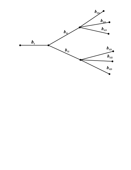
Figure 2: Tree graph.

Furthermore, we seek for the solution of Eq. (7) on the each bonds in the form

$$f_{b}=B_{b}sn\left(\alpha_{b}x+\delta_{b}\left|k_{b}\right.\right),$$

where $\delta_{b}$ are parameters that can be determined by the given boundary conditions: $\delta_{1}=0,\ \delta_{1ij}=-\alpha_{1ij}L_{1ij}$.

Again, as it was done in the previous section for star graph, one can show posibility of the exact solution for two special cases.

The first case is given by the relations

$$\frac{4n_{1}+1}{L_{1}}=\frac{4(n_{1i}^{(2)}-n_{1i}^{(1)})}{L_{1i}-L_{1}}=\frac{4n_{1ij}+1}{L_{1ij}-L_{1i}},\;i=1,2,\;j=1,2,3$$

where $n_{1},n_{1i},n_{1ij}\in{\bf N}\cup\{0\},n_{1i}^{(2)}>n_{1i}^{(1)}$ and

$$\alpha_{1}=\frac{4n_{1}+1}{L_{1}}K(k_{1}),\;\alpha_{1i}=\frac{4(n_{1i}^{(2)}-n_{1i}^{(1)})}{L_{1i}-L_{1}}K(k_{1i}),\;\alpha_{1ij}=\frac{4n_{1ij}+1}{L_{1ij}-L_{1i}}K(k_{1ij}),\delta_{1i}=\left(\frac{4(n_{1i}^{(1)}L_{1i}-n_{1i}^{(2)}L_{1})}{L_{1i}-L_{1}}+1\right)K(k_{1i}).$$

It is easy to show that the following relations are valid:

$$\alpha_{1}=\alpha_{1i}=\alpha_{1ij}=\alpha,\;k_{1}=k_{1i}=k_{1ij}=k,\ \sigma_{1}=\sigma_{1i}=1,\ \sigma_{1ij}=-1.$$

Furthermore, we have

$$g(k)\equiv 2\frac{(4n_{1}+1)^{2}}{L_{1}^{2}}\left\{\frac{L_{1}}{\beta_{1}}+\sum_{i=1}^{2}\left[\frac{L_{1i}-L_{1}}{\beta_{1i}}+\sum_{j=1}^{3}\frac{L_{1ij}-L_{1i}}{\beta_{1ij}}\right]\right\}K(k)\left(K(k)-E(k)\right)-1=0.$$

Solvability of the last equation is obvious.

The second case is given by the relations

$$\alpha_{1}=\frac{-(-1)^{n_{1}}p_{1}+2n_{1}K(k_{1})}{L_{1}},\;\alpha_{1i}=\frac{(-1)^{n_{1i}^{(2)}}p_{1i}-(-1)^{n_{1i}^{(1)}}p_{1}+2(n_{1i}^{(2)}-n_{1i}^{(1)})K(k_{1i})}{L_{1i}-L_{1}},\;$$

$$\alpha_{1ij}=\frac{-(-1)^{n_{1ij}}p_{1i}+2n_{1ij}K(k_{1ij})}{L_{1ij}-L_{1i}},$$

$$\delta_{1i}=\frac{(-1)^{n_{1i}^{(1)}}p_{1}L_{1i}-(-1)^{n_{1i}^{(2)}}p_{1i}L_{1}+2(n_{1i}^{(1)}L_{1i}-n_{1i}^{(2)}L_{1})K(k_{1i})}{L_{1i}-L_{1}},$$

where $0<p_{1}<2K(k_{1,1i}),\;0<p_{1i}<2K(k_{1i,1ij})$.

From vertex conditions we obtain

$$\alpha_{1}=\alpha_{1i}=\alpha_{1ij}=\alpha,\;k_{1}=k_{1i}=k_{1ij}=k$$

and

$$\frac{(-1)^{n_{1}}}{\beta_{1}}-\sum_{i=1}^{2}\frac{(-1)^{n_{1i}^{(1)}}}{\beta_{1i}}=0,\;\frac{(-1)^{n_{1i}^{(2)}}}{\beta_{1}}+\sum_{j=1}^{3}\frac{(-1)^{n_{1ij}}}{\beta_{1ij}}=0.$$

It follows from the normalization condition that

$$g(k)\equiv 4\left(\frac{(-1)^{n_{1}}p+2n_{1}K(k)}{L_{1}}\right)\left(\frac{n_{1}}{\beta_{1}}+\sum_{i=1}^{2}\left[\frac{n_{1i}^{(2)}-n_{1i}^{(1)}}{\beta_{1i}}+\sum_{j=1}^{3}\frac{n_{1ij}}{\beta_{1ij}}\right]\right)\left(K(k)-E(k)\right)-1=0.$$

Solvability of the last equation follows from the properties of the function $g(k)$.

IV.2 Graph With Loops

Similar results can be obtained in for the loop graph plotted in the Fig. 3.

The solution of Eq.(7) for this topology can be written in terms of the Jacobian elliptic functions as

$$f_{1}(x)=B_{1}sn\left(\alpha_{1}x|k_{1}\right),$$

$$f_{j}(x)=B_{j}sn\left(\alpha_{j}x+\delta_{j}|k_{j}\right),\;j=2,3,$$

$$f_{4}(x)=B_{4}sn\left(\alpha_{4}(x-L_{4})|k_{4}\right).$$

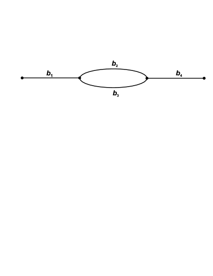
Figure 3: Loop graph.

Again, two special cases will be considered.

For the first case we put $\frac{4n_{1,4}+1}{L_{1,4}}=\frac{4(n_{2,3}^{(2)}-n_{2,3}^{(1)})}{L_{2,3}-L_{1}}$, where $n_{1,4},n_{2,3}^{(1),(2)}\in{\bf N}\cup\{0\}$, $n_{2,3}^{(2)}>n_{2,3}^{(1)}$. Choosing

$$\alpha_{1,4}=\frac{4n_{1,4}+1}{L1,4}K(k_{1,4}),\;\alpha_{2,3}=\frac{4(n_{2,3}^{(2)}-n_{2,3}^{(1)})}{L_{2,3}-L_{1}}K(k_{2,3}),$$

$$\delta_{2,3}=\left(\frac{4(n_{2,3}^{(1)}L_{2,3}-n_{2,3}^{(2)}L_{1})}{L_{2,3}-L_{1}}+1\right)K(k_{2,3}).$$

We have $\alpha_{j}=\alpha,\;k_{j}=k,j=1,2,3,4$, $\sigma_{1}=\sigma_{2}=\sigma_{3}=1,\ \sigma_{4}=-1$. From the normalization condition we get

$$g(k)\equiv 2\frac{(4n_{1}+1)^{2}}{L_{1}^{2}}\left\{\frac{L_{1}}{\beta_{1}}+\frac{L_{2}-L_{1}}{\beta_{2}}+\frac{L_{3}-L_{1}}{\beta_{3}}+\frac{L_{4}}{\beta_{4}}\right\}K(k)\left(K(k)-E(k)\right)-1=0.$$

The second case is given by

$$\alpha_{1}=\frac{(-1)^{n_{1}}p_{1}+2n_{1}K(k_{1})}{L_{1}},\;\alpha_{2,3}=\frac{(-1)^{n_{2,3}^{(2)}}p_{2}-(-1)^{n_{2,3}^{(1)}}p_{1}+2(n_{2,3}^{(2)}-n_{2,3}^{(1)})K(k_{2,3})}{L_{2,3}-L_{1}},$$

$$\alpha_{4}=\frac{(-1)^{n_{4}}p_{2}+2n_{4}K(k_{4})}{L_{4}},$$

$$\delta_{2,3}=\frac{(-1)^{n_{2,3}^{(1)}}p_{1}L_{2,3}-(-1)^{n_{2,3}^{(2)}}p_{2}L_{1}+2(n_{2,3}^{(1)}L_{2,3}-n_{2,3}^{(2)}L_{1})K(k_{2,3})}{L_{2,3}-L_{1}},$$

where $0<p_{1}<2K(k_{1,2,3}),\;0<p_{2}<2K(k_{2,3,4})$.

Then from the $\delta^{\prime\prime}-$type vertex conditions we obtain $\alpha_{j}=\alpha,\;k_{j}=k,j=1,2,3,4$ and

$$\frac{(-1)^{n_{1}}}{\beta_{1}}-\frac{(-1)^{n_{2}^{(1)}}}{\beta_{2}}-\frac{(-1)^{n_{3}^{(1)}}}{\beta_{3}}=0,\;\frac{(-1)^{n_{2}^{(2)}}}{\beta_{2}}+\frac{(-1)^{n_{3}^{(2)}}}{\beta_{3}}+\frac{(-1)^{n_{4}}}{\beta_{4}}=0.$$

Furthermore, according to the normalization condition one can obtain the following equation

$$g(k)\equiv 4\left(\frac{(-1)^{n_{1}}p+2n_{1}K(k)}{L_{1}}\right)\left(\frac{n_{1}}{\beta_{1}}+\sum_{i=2}^{3}\frac{n_{i}^{(2)}-n_{i}^{(1)}}{\beta_{i}}+\frac{n_{4}}{\beta_{4}}\right)\left(K(k)-E(k)\right)-1=0.$$

In both cases solvability of the equation $g(k)=0$ follows from the asymptotical relations, $\lim_{k\to 0}g(k)=-1,\;\lim_{k\to 1}g(k)=+\infty$ and from the continuity of the function $g(k)$.

V Conclusions

In this paper we have treated the stationary nonlinear Schrödinger equation with cubic nonlinearity for simplest graphs. Unlike the previous studies Zarif ; Adami ; Uzy4 , the lengths of the bonds are considered as finite. Therefore, our work can be considered as an extension of the results by L.D. Carr Car1 ; Car2 ; Car3 to the case of networks. Formulation of the problem and its detailed treatment including method for finding exact solutions are presented for the case of star graph consisting of three bonds. The method is extended for other simplest topologies such as tree and loop graphs. The cases of attractive and repulsive nonlinearities are treated separately. The above results can be useful for the problems of BEC on networks and discrete traps, soliton transport optical waveguide networks, soliton excitation in DNA double helix, energy transfer in nanoscale networks etc. In principle, the method developed in this work can be extended for more complicated topologies, too. Currently such a study is on progress.

References

• (1) Zakharov V E and Shabat Sov. Phys. JETP 34 62 (1972)
• (2) Zakharov V E and Shabat Funct. Anal. Appl. 8 226 (1974)
• (3) Zakharov V E and Shabat Funct. Anal. Appl. 13 166 (1979)
• (4) Y. S. Kivshar and G. P. Agarwal, Optical Solitons: From Fibers to Photonic Crystals (Academic, San Diego, 2003).
• (5) M.J. Ablowitz and P.A. Clarkson Solitons, Nonlinear Evolution Equations and Inverse Scattering (Cambridge: Cambridge University Press, 1999).
• (6) C. J. Pethick and H. Smith, Bose-Einstein Condensation in Dilute Gases (Cambridge University Press, Cambridge, England, 2002).
• (7) L.Pitaesvki and S. Stringari, Bose-Einstein Condensation (Oxford University Press, Oxford, England, 2003).
• (8) Thierry Dauxois, Michel Peyrard, Physics of Solitons (Cambridge University Press, Cambridge, England, 2006).
• (9) L. D. Carr, Charles W. Clark, & W. P.Reinhardt, Phys. Rev. A, 62, 063610 (2000).
• (10) L. D. Carr, Charles W. Clark, & W. P. Reinhardt, Phys. Rev. A, 62, 063611 (2000).
• (11) R. D Agosta, B. A. Malomed, and C. Presilla, Phys. Lett. A 275, 424, (2000).
• (12) L. D. Carr, K. W. Mahmud, and W. P. Reinhardt, Phys. Rev. A 64, 033603 (2001).
• (13) K. Rapedius, D. Witthaut, and H. J. Korsch, Phys. Rev. A 73, 033608 (2006).
• (14) E.Infeld, P.Zin, J.Gocalek, & M.Trippenbach, Phys. Rev. E, 74, 026610 (2006).
• (15) F. Harary, Graph Theory (Addison-Wesley, Reading, 1969).
• (16) Tsampikos Kottos and Uzy Smilansky, Ann.Phys., 76 274 (1999).
• (17) Sven Gnutzmann and Uzy Smilansky, Adv.Phys. 55 527 (2006).
• (18) S. GnutzmannJ.P. Keating b, F. Piotet, Ann.Phys., 325 2595 (2010).
• (19) P.Exner, P.Seba, P.Stovicek, J. Phys. A: Math. Gen. 21 4009-4019 (1988).
• (20) P.Exner, P.Seba, Rep. Math. Phys., 28 7 (1989).
• (21) S. Yomosa, Phys. Rev. A 27 , 2120 (1983).
• (22) C.T.Zhang, Phys. Rev. A 35 , 886 (1987).
• (23) L.V. Yakushevich, A.V. Savin, L.I. Manevitch, Phys. Rev. A 66 ,016614 (2002).
• (24) A.S. Davydov, Biology and Quantum Mechanics, (Oxford: Pergamon, 1982)
• (25) R. Burioni, D. Cassi, P. Sodano, A. Trombettoni, and A. Vezzani, Chaos 15, 043501 (2005); Physica D 216, 71 (2006).
• (26) P. Leboeuf and N. Pavloff, Phys. Rev. A 64 , 033602 (2001).
• (27) K. Bongs, et al. Phys. Rev. A 63 , 031602 (R) (2001).
• (28) J.A. Stickney, A.A. Zozulya, Phys. Rev. A 65, 053612 (2002).
• (29) O. Sotolongo-Costa1, G. J. Rodgers, Phys. Rev. E 68 , 056118 (2003).
• (30) T. Paul, P. Leboeuf, N. Pavloff, K. Richter, and P. Schlagheck, Phys. Rev. A 72, 063621 (2005).
• (31) T. Paul, M. Hartung, K. Richter, and P. Schlagheck, Phys. Rev. A 76, 063605 (2007).
• (32) I. N. de Oliveira, Phys. Rev. E 81 , 030104(R) (2010).
• (33) Z. Sobirov, D. Matrasulov, K. Sabirov, S. Sawada, and K. Nakamura, Phys. Rev. E 81 , 066602 (2010).
• (34) R.Adami, C.Cacciapuoti, D.Finco, D.N., Rev.Math.Phys, 23 4 (2011).
• (35) R.C. Cascaval, C.T. Hunter, Libertas Math. 30 85 (2010).
• (36) V. Banica, L.Ignat, Arxiv: 1103.0429.
• (37) S. Gnutzmann, U. Smilansky, S. Derevyanko, Phys. Rev. A 83 033831 (2011).
• (38) R.Adami, C.Cacciapuoti, D.Finco, D.N., Arxiv: 1104.3839.
• (39) R. Burioni, D. Cassi, P. Sodano, A. Trombettoni, and A. Vezzani, Phys. Rev. E 73 , 066624 (2006).
• (40) F. Bowman, Introduction to Elliptic Functions, with Applications (Dover, New York, 1961).