Massive Star-formation around IRAS 05345+3157
I: The Dense Gas

Abstract

We present observations of the intermediate to massive star-forming region I05345+3157 using the molecular line tracer CS($2-1$) with CARMA to reveal the properties of the dense gas cores. Seven gas cores are identified in the integrated intensity map of CS($2-1$). Among these, core 1 and core 3 have counterparts in the $\lambda$ = 2.7 mm continuum data. We suggest that core 1 and core 3 are star-forming cores that may already or will very soon harbor young massive protostars. The total masses of core 1 estimated from the LTE method and dust emission by assuming a gas-to-dust ratio are 5$\pm$1 M_☉ and 18$\pm$6 M_☉, and that of core 3 are 15$\pm$7 M_☉ and 11$\pm$3 M_☉. The spectrum of core 3 shows blue-skewed self-absorption, which suggests gas infall – a collapsing core. The observed broad linewidths of the seven gas cores indicate non-thermal motions. These non-thermal motions can be interactions with nearby outflows or due to the initial turbulence; the former is observed, while the role of initial turbulence is less certain. Finally, the virial masses of the gas cores are larger than the LTE masses, which for a bound core implies a requirement on the external pressure of $\sim 10^{8}$ K cm^-3. The cores have the potential to further form massive stars.

1 INTRODUCTION

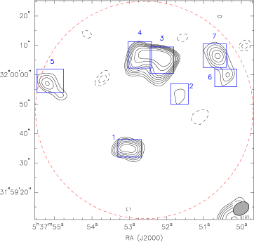
Figure 1: Contour map of CS $J=2-1$ integrated intensity with the FWHM beam size shown in the lower right corner. The dashed circle is the size of the primary beam of the 10-meter dishes. The synthesized beam size, shown in the right-bottom corner, is 4.3″$\times$5.9″with P.A.=-57.5°. The noise is 0.25 Jy beam^-1 km s^-1, and the contours are 5$\sigma$, 6$\sigma$, 7$\sigma$, 8$\sigma$, 9$\sigma$, 10$\sigma$, 12$\sigma$, 14$\sigma$, positive and negative. The boxes are drawn based on the 3$\sigma$ detections and are used to define cores.

Despite the well-known fact that most stars form in clusters (e.g., Lada & Lada, 2003), little is known about the detailed formation process of massive stars or star clusters. In contrast to the well-studied mechanisms for low mass star formation, the difficulty for massive star formation is mainly due to a massive star’s high radiative power. The strong radiation hinders infalling material in the envelope from further accreting onto the central source. Two major theories have been proposed to solve the puzzle. Accretion can still be accomplished through a high accretion rate generated by the turbulent environment (McKee & Tan, 2003) and also through disks (e.g. Krumholz et al., 2005) with outflows that greatly reduce the radiative pressure (Krumholz et al., 2005). On the other hand, massive stars could also form from competitive accretion or stellar mergers (Bonnell et al., 2001; Bonnell et al., 2004) in high stellar density regimes. The formation of star clusters can be due to fragmentation of molecular clouds (e.g., Bate & Bonnell, 2005), although Krumholz et al. (2007) concluded that the fragmentation of pre-stellar massive cores can be avoided through heating, allowing the formation of a massive star from one massive core. Only through a detailed investigation of the initial conditions in a protocluster system can we better address the problem of massive star formation.

Massive protostars have strong interactions with their ambient environment. They disperse their natal clouds through stellar winds and UV radiation (see the review by Zinnecker & Yorke, 2007). After such dynamical interactions, the ambient environment changes enormously and no longer preserves the initial conditions from when massive protostars were first born. Therefore, in order to examine the very early conditions of the onset of massive star formation, identifying stellar objects at early evolutionary stages (e.g., Seale et al., 2009) in protoclusters appears to be very essential. Beuther et al. (2007) suggested that the early evolution has four stages starting with High-Mass Starless Cores (HMSCs), which then accrete low and intermediate mass protostars, leading to High-Mass Protostellar Objects (HMPOs) and finally the (still deeply embedded) final star.

Here we report on the massive star-forming region around the FIR-bright IRAS source 05345+3157, hereafter I05345. The IRAS source is associated with an IR cluster surrounded by molecular gas at a distance of 1.8 kpc (Henning et al., 1992). HCO⁺(2-1) emission east of I05345 presents complex and clumpy structures, suggesting that the source is on the verge of collapse through the contraction of local density peaks (Molinari et al., 2002). A massive outflow has been observed in CO(2-1) (Zhang et al., 2005; Fontani et al., 2009), a typical signature of young stellar objects. Klein et al. (2005) shows a ring of dust emission around the cluster I05345 in 850 $\micron$ continuum data. Two compact and massive dust clumps are located in the ring to the east of the cluster: I05345 #1 and #2, with the mass of 48 M_☉ and 38 M_☉, respectively. Futhermore, Fontani et al. (2008) and Fontani et al. (2009) concluded several objects at different evolutionary stages in this region with SMA and PdBI observations, including prestellar core candidates, young intermediate to high mass class 0 protostars, and an early-B ZAMS star. The same papers also revealed two condensations in N₂D⁺(2-1) and the nature of the deuterated cores have been studied in detail.

The previous observations showed the possibility of active star formation in I05345. The main goal of this paper is to study star formation by investigating the dense gas in the I05345 environment. Our strategy uses the CS($2-1$) transition as a probe of gas cores to comprehensively study gas properties. We use the D array configuration of the Combined Array for Research in Millimeter-wave Astronomy (CARMA) to resolve-out large-scale structures and trace dense gas fragments ($\sim$ 10⁵ cm^-3) inside the cloud. In this paper we present $\sim$5″ angular resolution data of CS($2-1$) and 2.7 mm continuum. In the companion paper by Klein et al. (2011) (hereafter paper II), we examine the infrared properties of the fragments. With the two papers, we obtain a general picture of star formation in I05345.

2 OBSERVATIONS

2.1 CARMA observations

Observations of the line transition CS $J=2\rightarrow 1$ ($\nu=97.981$ GHz) toward the clumps I05345 #1 and #2 (Klein et al., 2005) were made with CARMA in 2008 June. The observations used CARMA D array at $\lambda=2.7$ mm. The CS($2-1$) transition was placed in a correlator window of 8 MHz width and a velocity resolution of 0.37 km s^-1. Two 500 MHz bands were set up for continuum observations. The phase center was chosen between I05345 #1 and #2 at $RA=05^{\text{h}}37^{\text{m}}52.6^{\text{s}}$ and $DEC=+31^{\circ}59\arcmin 48.0\arcsec$ (J2000) using the local standard of rest velocity V${}_{\text{LSR}}$ of $-18.6$ km s^-1 (Schreyer et al., 1996). 0555+398 was used as the phase calibrator. 3C454.3 and Uranus were used for the bandpass calibration and the flux calibration, respectively. The system temperature ranged from 50 K to 300 K with 200 K (single sideband) being a representative value. The baselines ranged from 11 meters to 150 meters. The channel maps were generated with natural weighting, producing a synthesized beam of $5.7\arcsec\times 4.2\arcsec$. The primary beam size of the CARMA combined array is 85″at 98 GHz. The data reduction was done using the MIRIAD package (Sault et al., 1995). The amplitude calibration is estimated to be 10%, and the uncertainties discussed afterwards are only statistical not systematic.

3 RESULTS

3.1 CS Zeroth Moment Map and Spectra

Table 1: Parameters of the identified cores

Label	R.A.	Dec.	$a_{0}$	$b_{0}$	P.A.0	a	b	P.A.	R
	(J2000.0)	(J2000.0)	(arcsec)	(arcsec)	(deg)	(arcsec)	(arcsec)	(deg)	(10-2 pc)
Core 1	05:37:53.03	31:59:34.9	$12.0\pm 1.6$	$6.9\pm 0.6$	$+83.5\pm 5.3$	$10.9\pm 1.8$	$4.9\pm 0.8$	78.8	$3.2\pm 0.4$
Core 2	05:37:51.67	31:59:53.0	$8.8\pm 2.2$	$7.5\pm 1.7$	$-25.4\pm 55.6$	$7.2\pm 2.4$	$5.5\pm 2.3$	-3.7	$2.7\pm 0.7$
Core 3	05:37:52.19	32:00:05.4	$12.3\pm 3.9$	$8.9\pm 1.5$	$+63.9\pm 27.3$	$11.4\pm 4.2$	$7.0\pm 1.9$	58.8	$3.9\pm 0.9$
Core 4	05:37:52.58	32:00:06.5	$11.8\pm 4.0$	$7.4\pm 1.2$	$-83.6\pm 14.9$	$10.5\pm 4.5$	$5.9\pm 1.5$	-88.3	$3.4\pm 0.9$
Core 5	05:37:55.14	31:59:57.0	$12.3\pm 2.6$	$8.1\pm 1.0$	$+48.2\pm 17.2$	$11.5\pm 2.8$	$5.9\pm 1.4$	45.6	$3.6\pm 0.6$
Core 6	05:37:50.39	32:00:01.0	$11.8\pm 7.9$	$6.8\pm 1.3$	$-14.2\pm 20.7$	$10.7\pm 8.7$	$4.6\pm 1.9$	-9.3	$3.1\pm 1.4$
Core 7	05:37:50.64	32:00:06.3	$11.1\pm 0.9$	$7.7\pm 0.4$	$+37.2\pm 7.7$	$10.3\pm 1.0$	$5.1\pm 0.6$	36.0	$3.2\pm 0.2$

a₀, b₀ and P.A.₀ are the observed major axis, minor axis and position angle of the cores. a, b and P.A. are the deconvolved major axis, minor axis and position angle. R is the equivalent radius, $Sqrt{ab}/2$.

Figure 1 shows the velocity-integrated intensity map of CS($2-1$); the dashed circle is approximately the primary beam size of the 10-m antennas in CARMA ($\sim 69\arcsec$) at $\lambda$=2.7 mm. We identify seven cores with peak intensities above $5\sigma$ (1 $\sigma$ $\sim$ 0.25 Jy beam${}^{\text{-1}}$ km s${}^{\text{-1}}$) inside the primary beam of the integrated CS map . Due to the interferometric effect that introduces the negative components in the map, it is possible that the weak emission associated with core 2 is spurious. The boxes shown in the right panel of Figure 1 are used for deriving the parameters of the cores (see the paragraph below) and are drawn based on the 3$\sigma$ detection.

For this study, we only focus on the cores inside the primary beam size of the 10-m OVRO dishes and neglect the emission outside the primary beam, which has a lower sensitivity and signal-to-noise ratio. Core 1 is isolated in the south. Cores 3 and 4 are spatially close and entangled. In Table 1 the parameters of each core are specified, including the observed sizes (major axis a₀, minor axis b₀ and position angle P.A.₀), the deconvolved sizes (major axis a, minor axis b and position angle P.A.) and the equivalent radius R=$\sqrt{ab}/2$. The major and minor axes are derived by fitting a circular or elliptical Gaussian profile in the velocity-integrated map of CS. At the distance of 1.8 kpc, the sizes of these cores range from 0.05 pc to 0.08 pc (see Table 1), which is the typical size of transition groups from Hot Molecular Cores (HMCs) to Ultracompact HII regions (UCHIIs) (Beuther et al., 2007) or of low-mass envelopes (e.g., Looney et al., 2000).

The spectra of the seven cores averaged over the boxes in Figure 1 are shown in Figure 2. Most of the spectra show a strong single-peaked emission, while the spectra of core 2 and 3 are double peaked. The spectra are fitted by Gaussian profiles as shown in Figure 2. Since the double peaks in the spectra of core 2 and core 3 may result from self-absorption (Sect. 4.1), we fit the profiles with one Gaussian emission and one Gaussian absorption line superimposed. Table 2 lists the fitting parameters for each core (amplitude, peak position of velocity, FWHM). Note that the spectrum of core 4 shows a red wing emission and that of clump 6 shows a blue wing emission above the fitted line. The line wings may be due to the outflow driven by core 3 (see Sect. 4.2).

3.2 Millimeter Continuum Data

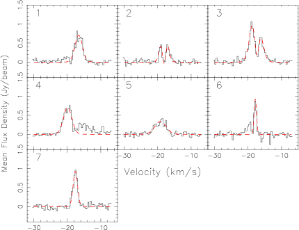
Figure 2: Spectra of identified CS cores. V_LSR is -18.6 km/s. The dashed lines are the best fit Gaussians.

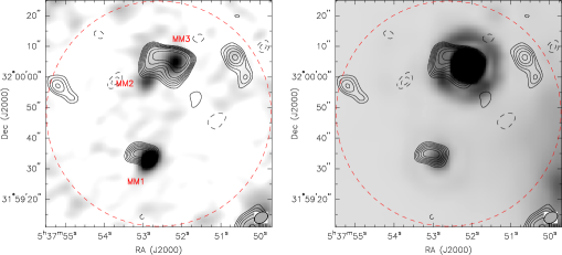
Figure 3: Left panel: CS($2-1$) emission overlaid on the gray-scale 2.7 mm continuum data. The contours represent the CS integrated intensity with the same contour levels with Fig. 1. Right panel: CS($2-1$) emission overlaid on the gray-scale Spitzer 24 $\micron$ data. The contours are the same as in the left panel.

Figure 3 shows the contours of the CS intensity map overlaid on the 2.7 mm continuum data from the same observation. There are three 2.7 mm continuum emission peaks in the map (MM1, MM2 and MM3). MM1 in the south is the brightest core ($22.7\pm 7.2$ mJy). MM2, the faintest ($6.0\pm 1.4$ mJy), is in the north accompanied by the brighter MM3 ($13.8\pm 3.6$ mJy). These sources are all unresolved.

Comparing the $\lambda$=2.7 mm observation with CS cores, we see that core 1 is associated with MM1 although the two peaks are shifted by about 3$\arcsec$, smaller than the beam size. Core 3 coincides with MM3, while MM2 shows no CS emission (see below). There are no other 2.7 mm emission features associated with the rest of the CS cores.

MM3 and MM1 correspond to the clumps I05345 #1 and #2 for which Klein et al. (2005) derived masses of 48 M_☉ and 38 M_☉, respectively. Cores 2, 3 and 4 are all associated with the northern clump I05345 #1. In addition, the three cores C1, C2, and C3 in 225 GHz continuum observation by Fontani et al. (2008) coincide with MM3, MM2, and MM1, respectively.

The cores MM1 and MM3 have been consistently detected in the (sub-)millimeter continuum and also in the FIR by Spitzer (see paper II for details). Figure 3 shows the Spitzer 24 $\micron$ image; the bright northern source corresponds to our core 3 and the southern source corresponds to core 1. It is peculiar that at 2.7 mm the northern source is the weaker one of the two while at all other wavelengths from 24 µm to 1.3 mm (the 225 GHz observation in Fontani et al. (2008)) the northern source is the dominant source. We speculate that there is extended emission that contributed to the single-dish observation by Klein et al. (2005), which is resolved out by the interferometer. Thus, the fluxes seen by the interferometer are smaller than expected from the single-dish observations, and one would expect that the effect is more pronounced for the larger core MM3.

MM2 shows no counterpart at 850 $\mu$m or in the FIR, but it does have a counterpart at 3.6 cm (Molinari et al., 2002); therefore, the continuum emission from core MM2 is likely dominated by free-free emission from an Hii-region with only a fraction of the emission from warm dust.

3.3 Estimating the Core Mass

We present three approaches to roughly estimate the core masses. The first method is the LTE mass calculated from the integrated flux of the CS($2-1$) line transition. The second method is calculating the virial mass from the line width of CS spectra. The third method is based on the 2.7 mm continuum assuming dust emission and a dust-to-gas ratio.

3.3.1 LTE Mass

Following the standard rotation temperature - column density analysis (e.g., Turner, 1991), CS($2-1$) spectra can be used to derive the column density, and further the mass of the dense gas. Because the transition CS($2-1$) is not optically thin, a correction factor needs to be applied to the LTE mass derived from the assumption of an optically thin line. For an optically thin molecular line, by assuming all the transitions are excited by a single temperature T${}_{\text{ex}}$ (LTE) and negligible background continuum emission, the column density can be calculated from (e.g., Miao et al., 1995; Mehringer, 1995)

$$\begin{split}{\text{N}}\ (cm^{-2})=&2.04\times 10^{20}\times[\frac{1}{\theta_{a}\theta_{b}(arcsec^{2})}]\\ &\times[\frac{Qe^{E_{u}(K)/T_{ex}}}{\nu^{3}(GHz^{3})S\mu^{2}(debye^{2})g_{k}g_{I}}]\\ &\times[\int I(Jy\ beam^{-1})dv(km\ s^{-1})]\ ,\end{split}$$

where $\theta_{a}$ and $\theta_{b}$ are the FWHM of the synthesized beam, Q is the partition function, E${}_{\text{u}}$ is the upper energy level of the transition, $\nu$ is the line rest frequency, S is the line strength, and $\mu^{2}$ is the dipole moment, $g_{k}$ and $g_{I}$ are the usual K-level and reduced nuclear spin degeneracies. For our observation, $\theta_{a}$=5.9$\arcsec$, $\theta_{b}$=4.3$\arcsec$, Q=0.86T${}_{\text{ex}}$ (Rohlfs & Wilson, 2000), E${}_{\text{u}}$=7.05 K, $\nu$=97.980968 GHz, S=2, $\mu$=1.96 debye, and $g_{I}$=$g_{k}$=1. Here we assume an excitation temperature of 20 K for dense cores forming massive stars (see review by Zinnecker & Yorke, 2007). In the case of an optically thick molecular line, a correction factor C_τ should be applied (e.g., Goldsmith & Langer, 1999):

$$\text{N}_{\text{total}}=C_{\tau}\text{N}\ \text{and}$$

$$C_{\tau}=\frac{\tau}{1-e^{-\tau}}\ ,$$

where $\tau$ is the optical depth and can be derived from

$$\tau=-\ln[1-\frac{T_{MB}}{J(T_{\text{ex}})-J(2.73)}]$$

(Rohlfs & Wilson, 2000), where T${}_{\text{MB}}$ is the main beam brightness temperature and

$$J(T)=\frac{h\mu}{k}\frac{1}{e^{h\mu/kT}-1}.$$

Therefore, by assuming uniform densities, the LTE mass can be derived from

$$M=\mu m_{H}\frac{N}{X}(1.133abD^{2})$$

where $\mu=2.33$ is the mean molecular weight, $m_{H}$ is hydrogen mass, D is the distance (1.8 kpc for I05345), X is the abundance ratio of CS to H₂, which is assumed to be 10^-9 here (Rohlfs & Wilson, 2000), and $a$ and $b$ are the major axis and minor axis of a defined core. Furthermore, we calculated the number density of molecular hydrogen for these cores by assuming ellipsoidal cores and $a,\ b$ and $b$ for the three axes: n${}_{H_{2}}$ = $M_{LTE}/2M_{H}/(4\pi/3(a/2)(b/2)^{2})$. The column density and number density of H₂ range from $2.7\times 10^{22}$ to $11.6\times 10^{22}$ cm^-2, and from $0.6\times 10^{6}$ to $1.7\times 10^{6}$ cm^-3, respectively. The LTE masses of the different cores range from $\sim$ 2 M_☉ to 15 M_☉. Table 3 lists the integrated line intensity ($I_{t}=\int Idv$), the derived optical depth $\tau$, the column density of CS (N_CS), the number density of H₂ and the results of LTE mass.

The smallest core mass that our observations are sensitive to is $\sim$ 1 M_☉. This is the result of the same calculation as above assuming a flux equivalent to $3\sigma$ in integrated flux map. Fontani et al. (2009) observed their condensations N and S in N₂D⁺ and N₂H⁺ and expected them to be low-mass cores ($<1\,M_{\sun}$) according to the observed deuterium fraction. Thus, it is not surprising that we don’t detect their condensations N and S.

In the calculation of the LTE masses, a value of 10^-9 for the CS(2-1) molecular abundance is assumed and the abundance is also assumed to be a constant. However, due to C-bearing molecules frozen onto dust grains at early stages of star formation, a central depletion of CS(2-1) is usually seen in prestellar cores (e.g. Tafalla et al., 2002; Stahler & Yen, 2010), and therefore the assumption of a constant abundance may lead to larger uncertainties in the calculation. Also, according to different models or calculations, the derived values for CS(2-1) abundance are various (e.g. Belloche et al., 2002; Pirogov et al., 2007). In most literatures, the abundance profile is described by a central depletion and a nearly constant value between 10^-9 and 10^-8 follows at outer parts of cores. Since the radii where the abundance drops is usually very close to the center of prestellar cores, we simplify the LTE mass estimation by only adopting the plateau part of the molecular abundance. The choice of 10^-9 sets the upper limit for the calculation and the derived LTE masses could vary by about one order of magnitude depending on the chosen values for the abundance.

Table 2: Fitting Parameters For Cores

Label	Amplitude	Peak Position	FWHM
	Jy/beam	km/s	km/s
Core 1	$0.704\pm 0.002$	$-16.592\pm 0.004$	$2.626\pm 0.009$
Core 2	$2.008\pm 0.380$	$-18.065\pm 0.004$	$1.987\pm 0.053$
	$-2.040\pm 0.379$	$-18.071\pm 0.004$	$1.480\pm 0.045$
Core 3	$1.749\pm 0.032$	$-17.659\pm 0.005$	$3.237\pm 0.018$
	$-1.524\pm 0.031$	$-17.441\pm 0.003$	$1.735\pm 0.016$
Core 4	$0.699\pm 0.003$	$-19.894\pm 0.006$	$2.983\pm 0.015$
Core 5	$0.337\pm 0.002$	$-19.172\pm 0.012$	$3.940\pm 0.029$
Core 6	$0.922\pm 0.047$	$-17.832\pm 0.021$	$0.849\pm 0.049$
Core 7	$0.921\pm 0.003$	$-17.600\pm 0.003$	$1.584\pm 0.007$

3.3.2 Virial Mass

By assuming the cores are in virial equilibrium, we can derive the virial mass using the line width of CS. We assume a standard isothermal density profile for the cores from Shu (1977), $\rho=\rho_{0}r^{-2}$ (cf. Looney et al., 2003). In this case, the virial mass can be derived from

$$M_{vir}\sim\frac{3R}{G}\frac{\Delta V^{2}}{8\ln 2}\ ,$$

where $\Delta V$ is the FWHM of the observed molecular line (see Table 2). The derived virial mass for each core is listed in Table 3. For core 2 and 3 with the double-peak spectrum, we use the line width of the emission line to derive the virial masses.

3.3.3 Total Mass Estimation from Continuum Emission

Here we adopt the standard technique to estimate the total mass from the continuum emission, in our case the 2.7 mm continuum data for core 1 and 3 (remember that core 2 could have considerable free-free emission; Sect. 3.2). This method assumes that the continuum emission is from dust and a dust-to-gas ratio. By assuming optically thin emission and a single temperature (isothermal), the total mass (dust + gas) is

$$M=\frac{F_{\nu}D^{2}R}{B_{\nu}(T_{dust})\kappa_{\nu}}$$

where F_ν is the flux density, D is the distance to the source, R is the gas-to-dust ratio, B${}_{\nu}(T_{dust})$ is the Planck function at dust temperature T_dust, and $\kappa_{\nu}$ is the dust opacity. The flux density of core 1 is $22.7\pm 7.2$ mJy and that of core 3 is $13.8\pm 3.6$ mJy. For the dust opacity, assuming a gas density $\sim$ 10⁶ cm${}^{\text{-3}}$, we adopt the extrapolated value of 0.29 cm² g^-1 at $\lambda$=2.7 mm for prestellar core dust with thin ice mantles from Ossenkopf & Henning (1994). The extrapolation was done with a power law ($\kappa\propto\lambda^{-\beta}$) and a value of $\beta=1.77$, obtained by fitting the respective $\kappa$-values in the FIR ($\lambda>300\micron$). Therefore, with the assumption of 20 K for the dust temperature and 100 for the gas-to-dust ratio, we derive the mass of $18\pm 6\,M_{\sun}$ for core 1 and $11\pm 3\,M_{\sun}$ for core 3. The derived masses depend much on the assumed values for the dust temperature, the opacity, and the dust-to-gas ratio. The error of the mass estimates given above only reflects the uncertainty in the flux measurement. Taking the uncertainties of the assumptions into account the estimate is good within one order of magnitude. For example, if we would assume a rather high temperature of 47 K (Paper II) for core 3 the core mass would only be $7\,M_{\sun}$. If we would use the opacity for dust grains without ice mantels the mass would also drop to $7\,M_{\sun}$.

The calculation shows that the total mass from the LTE method and continuum emission of core 1 and core 3 are (5$\pm$1 M_☉, 18$\pm$6 M_☉) and (15$\pm$7 M_☉, 11$\pm$3 M_☉), respectively. Both methods have uncertainties. For example, the results depend on the assumptions of physical conditions and quantities, such as the excitation and dust temperature, wavelength dependence of the dust opacity etc. In CS(2-1) emission, core 3 is brighter than core 1, while it is opposite in the 2.7 mm continuum emission (see section 3.1 and  3.2). This result causes the larger LTE mass of core 3 and larger mass by assuming a dust-to-gas ratio of core 1. Other mid-infrared to FIR observations (see paper II) show a brighter core 3 than core 1, consistent with our CS(2-1) observation. Therefore, in the following discussion, we use the LTE mass to compare it with the virial mass, a method consistent with Saito et al. (2006).

4 DISCUSSION

4.1 A Collapsing Core

Figure 4 shows two CS($2-1$) integrated intensity maps integrated over velocities of the blue and red components of the self-absorption spectrum of core 3. The boxes drawn in these two maps are the same box as in Fig 1. Both of the integrated intensities from the blue and red peak are in the same box.

Arguably, this result suggests that the double-peak structure comes from the same core at the limit of our resolution (5$\arcsec$), although we cannot eliminate the possibility of two cores along the line of sight. However, the Gaussian fits in Table 2 (emission + absorption) describe the line feature of core 3 considerably well and provide an explanation to the double-peaked spectrum as coming from one core and showing self-absorption. Moreover, the absorption is close to the systemic velocity (Fontani et al., 2009) strengthening the evidence for self-absorption. However, it is important to note that the negative components in the map are not causing the self-absorption dip as the negative components seen in Fig 1 are not relevant in the box of core 3. To be more specific, we carefully examined the channel maps and there are only few negative contours in the channel where the deepest dip occurs (in the velocity of $\sim$ -17 km/s). Also, we mapped with short-spacing data removed and only very few negative contours remained, and the deep dip is still seen. As a result, the negative contours cannot be the main cause of the dip.

The double-peaked spectrum of core 3 shows one of the typical characteristics of gas infall motions: an optically thick transition (CS($2-1$) in our case) produces a blue-shifted, asymmetrical profile and central dip, with the blue-shifted line brighter than the red-shifted line (e.g., Zhou et al., 1993; Choi et al., 1995). This double-peaked feature is due to a temperature gradient and velocity gradient between each layer in a collapsing core (e.g., $v(r)\sim r^{-0.5}$ for the inside-out model) with a static envelope producing the central self-absorption dip. The blue-shifted line comes from the back side of the core and the red-shifted line from the front of the core. The lines with higher critical density and higher excitation temperature near the center will be obscured by the nearby lines with lower critical density and excitation temperature in the red peak, resulting in a stronger blue peak than red peak (Evans, 1999). In this case of I05345, optically thin lines peak in the dip of the self-absorbed lines. The absorption peaks approximately at the systemic velocity, also verified by optically thin tracers measured by Fontani et al. (2009).

Similar double-peaked profiles have been observed in CS($2-1$) for different objects (e.g., Choi et al., 1995; Tafalla et al., 1998; Belloche et al., 2002). However, the separation between the blue peak and the red peak in our observation is significantly larger ($\sim$ 3 km/s) than the separation in these studies ($\la$ 1 km/s). This broad separation may arise from the larger infall velocity for intermediate mass to massive protostars (e.g. Xue & Wu, 2008). The absorption feature in the envelope may also affect the separation of the two peaks. In addition, similar double-peaked profiles can be produced by a rotating core (Pavlyuchenkov et al., 2008). Detailed fitting with radiative transfer models is necessary to better understand other dynamics effects (turbulence, rotation etc.) in double-peaked profiles (Belloche et al., 2002).

Although core 2 also shows two peaks in the spectrum, the nature of core 2 is less understood. The asymmetry in the spectrum of the two peaks is not significant, indicating that the gas is less likely to be infalling. The dip is close to the systemic velocity, suggesting that the double-peaked feature may be caused by the self-absorption, while the fidelity of core 2 may be affected by the interferometric effect.

4.2 Dynamics of Cores

Table 3: Physical Properties of CS Cores

Label	It	$\tau$	NCS	n${}_{H_{2}}$	$\Sigma_{H_{2}}$	MLTE	Mvir	Pex/k
	(Jy/beam km/s)		($\times$1013 cm-2)	($\times 10^{6}$ cm-3)	(g cm-2)	(M☉)	(M☉)	(K cm-3)
Core 1	$1.94\pm 0.01$	$0.24$	$6.12\pm 0.03$	1.28$\pm 0.47$	$0.20\pm 0.00$	$5.3\pm 1.2$	$26.8\pm 3.4$	2.28$\times 10^{8}$
Core 2	$1.02\pm 1.00$	$0.21$	$3.17\pm 3.11$	0.59$\pm 0.53$	$0.11\pm 0.10$	$2.0\pm 2.3$	$13.2\pm 3.4$	0.84$\times 10^{8}$
Core 3	$3.30\pm 0.13$	$0.46$	$11.55\pm 0.46$	1.69$\pm 1.11$	$0.39\pm 0.02$	$14.8\pm 6.8$	$49.8\pm 11.5$	4.97$\times 10^{8}$
Core 4	$2.19\pm 0.01$	$0.27$	$7.01\pm 0.03$	1.22$\pm 0.81$	$0.23\pm 0.00$	$7.0\pm 3.5$	$37.1\pm 9.7$	3.24$\times 10^{8}$
Core 5	$1.39\pm 0.01$	$0.20$	$4.29\pm 0.03$	0.74$\pm 0.40$	$0.14\pm 0.00$	$4.7\pm 1.6$	$67.9\pm 11.4$	3.46$\times 10^{8}$
Core 6	$0.82\pm 0.06$	$0.36$	$2.73\pm 0.20$	0.61$\pm 0.70$	$0.09\pm 0.01$	$2.2\pm 2.0$	$2.7\pm 1.3$	0.06$\times 10^{8}$
Core 7	$1.53\pm 0.01$	$0.38$	$5.15\pm 0.03$	1.04$\pm 0.26$	$0.17\pm 0.00$	$4.4\pm 0.7$	$9.6\pm 0.6$	0.56$\times 10^{8}$

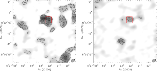
Figure 4: Maps of CS ($2-1$) integrated intensity of the blue and red part of the self-absorbed line of core 3. Left panel: The map of the blue emission peak. The integrated velocities range from -21.6 km s^-1 to -17.5 km s^-1. The contour levels start from 5$\sigma$ ($\sigma=0.12$ Jy beam^-1) and end at 28.3$\sigma$ with a logarithmic step of log($\sqrt{2}\sigma$). Right panel: The map of the right emission peak. The integrated velocities range from -17.1 km s^-1 to -14.9 km s^-1. The contour levels also start from 5$\sigma$ ($\sigma$=0.18 Jy beam^-1) and end at 28.3 $\sigma$ with a logarithmic step of log($\sqrt{2}\sigma$). The negative contours are not shown for simplicity.

Compared with the line widths for cores in other low-mass star forming regions (e.g., Onishi et al., 2002), we observe relatively large line widths from 1.5 km/s to 3.9 km/s for these seven cores. The isothermal sound speed for a region with a temperature 20 K is $\sim$ 0.27 km/s, much smaller than the observed line widths. Therefore, other non-thermal motions play a large role in the observed broad line widths. There are two possibilities for this non-thermal line-broadening (Saito et al., 2006). One possibility is that these cores formed from rather turbulent gas and still are turbulent. The other explanation is that the lines are broadened by interactions with the outflow or stellar wind from central protostars.

If initial large internal motions played a role in forming cores, higher density is necessary for a core to bind the system with gravitational energy. Saito et al. (2006) suggested such a possible correlation between line widths and the average H₂ density: the larger the line width, the higher the average density. Here we did not take the overall line widths of core 2 and 3 into consideration since their line widths may be affected and broadened by infall motions as discussed above. We see a weak trend (density vs. line widths) between core 1, 6 and 7. The line widths and average H₂ density of core 1, 6 and 7 are $2.63\pm 0.01$, $0.85\pm 0.05$, $1.58\pm 0.01$ km/s and $(1.28\pm 0.47)\times 10^{6}$, $(0.61\pm 0.70)\times 10^{6}$, $(1.04\pm 0.26)\times 10^{6}$ cm^-3, respectively. However, considering the large uncertainties in the data, the positive trend is less obvious and it is not clear about the role of the initial turbulence to the formation of the cores in this region from our data.

Core 4 and 5 do not follow the relation between the averaged density and line widths. Fontani et al. (2009) detected an outflow oriented in the west-east direction possibly driven by the 226 GHz continuum source C1-b or C1-a, which corresponds to our core 3. The same paper also indicated that this outflow is probably interacting with the southern portion of the highly deuterated condensation N, which corresponds to our core 4, and causes the observed broad lines. Therefore, the line width of core 4 is more possibly influenced by the interaction with the outflow. The red-wing emission of core 4 and the blue-wing emission of core 6 may result from the red and blue lobes of the outflow. Nevertheless, it is less clear about the mechanism for core 5 to produce the observed spectrum.

However, it seems that the gravitational energy is not enough to bind the systems. The derived virial masses are noticeably larger than the LTE masses except for core 6 (see Table LABEL:tbl:properties). Wang et al. (2008) studied low to intermediate mass cores around MWC 1080 with CS(2-1) and obtained similar LTE masses (calculated from the same method as described in Section 3.3.1) and virial masses. Saito et al. (2006) also concluded that non-turbulent cores have a similar virial mass to LTE mass but that the virial masses are usually larger than the LTE masses for turbulent cores. The line width of core 6 is similar to that of non-turbulent cores ($\sim$ 0.90 km/s average) and the similarity between its virial and LTE mass indicates that this core is bound by gravitational energy. On the other hand, for cores with a larger virial mass than LTE mass, external pressure must be applied to maintain a bound core. The virial equilibrium with an external pressure (by neglecting magnetic fields and rotation) can be expressed as:

$$0=2U+\Omega-4\pi R^{3}P_{ex}\ ,$$

where U=$\frac{1}{2}M\sigma^{2}$ ($\sigma$: velocity dispersion) is the kinetic energy and $\Omega=-\frac{3}{5}\frac{GM^{2}}{R}$ is the gravitational energy. The results of P_ex is listed in Table LABEL:tbl:properties. Except core 6, which is already gravitationally bound, other cores need an external pressure P_ex/k $\sim$ $10^{8}$ K cm^-3 to help maintain the structure of the cores. With the choice of higher molecular abundance by one order of magnitude, the external pressure needed to maintain the cores would decrease to $\sim$ $10^{7}$ K cm^-3. Observations have shown that such pressure is observed in several massive star-forming regions (e.g., McKee & Tan, 2003, and references therein). Therefore, we suggest that these turbulent cores with larger kinetic energy may still be bound by the external pressure.

4.3 Implication for Massive Star Formation

We suggest that core 3 and core 1 are young stellar objects. They show many indicators of high-mass star formation. Since young stellar objects are surrounded by dust and gas, they are not able to be revealed by optical observations (and shorter wavelength observations) due to dust extinction. Consequently, YSOs are often identified by their IR emission excess. The detection in the Spitzer 24 $\micron$ band is often an indicator of YSOs (e.g., Caulet et al., 2008). We observed an infrared counterpart of core 3 and 1 in the Spitzer image (Paper II), implying that both cores contain warm dust, suggestive of a YSO candidate. In addition, the CS spectrum of core 3 shows the typical signature of infalling gas motion — a double-peak feature with the stronger blue-shifted emission than the red-shifted emission. The wide separation of the two peaks ($\sim$ 3 km/s) is probably due to the higher masses.

Gas infall is also suggested by fitting the core’s SED with a radiative-transfer model in the companion paper (Paper II). The radiative-transfer modeling indicates that cores 3 and 1 could be an accreting stellar source with the central stellar mass of $\sim 5\,M_{\sun}$ surrounded by an envelope with a mass of order of $10\,M_{\sun}$ (mass estimates in this paper for core 3: $11\,M_{\sun}$ (dust mass), $17\,M_{\sun}$ (LTE mass) and core 1: 4 M_☉ (LTE mass), 18 M_☉ (dust mass)).

Although, the virial masses (20 and 50 M_☉ for core 1 and 3, respectively) are large compared to the LTE masses (4 and 20 M_☉), indicating that the cores may be gravitationally unbound, the cores can still be bound through the support of the external pressure. Therefore, core 3 and 1 are possibly accreting the envelope to form a star and potentially becoming a massive star ($M_{*}>8\,M_{\sun}$).

According to the classification of evolutionary stages of individual high-mass stars in Beuther et al. (2007), the formation of massive stars start with High-Mass Starless Cores (HMSCs) and then form High-Mass Protostellar Objects (HMPOs) via harboring or accreting low/intermediate-mass protostars. HMPOs are accreting high-mass protostars with masses larger than 8 M_☉, and consist of Hot Molecular Core (HMC), Hypercompact HII regions (HCHIIs, size $\leq$ 0.01 pc) and Ultracompact HII regions (UCHII regions, size $\leq$ 0.1 pc) at their early phases. Given the sizes of core 1 and core 3 (0.06 pc $\sim$ 0.08 pc) and the fact that the spectra of core 1 and 3 still peak in the far-infrared and have not approached near-infrared regimes, we suggest that these two cores are possibly on their way to become HMPOs.

Also, our cores are consistent with the massive star formation model proposed by McKee & Tan (2003). The theory states that turbulent cores in massive star-forming regions with pressure P_ex $\simeq$ $10^{8}\sim 10^{9}$ K cm^-3 can be gravitationally bound and form stars with high accretion rates ($10^{-3}$ M_☉ yr^-1) in a short time scale (several times the free-fall time). Our cores appear to be turbulent and non-thermal with line widths ranging from 1.5 km/s to 3.9 km/s. However, while the positive correlation between the line widths and average H₂ density implies that the initial turbulence may also influence the formation of these cores, such correlation is not obvious in our data considering the uncertainties. For core 3 and 4, the broad line widths may be also contributed by the outflow driven by core 3. With the exception of core 6, the cores have a larger virial mass than LTE mass. With the help of external pressure in the parent cloud, these turbulent cores can be bound and have the potential to become seeds for collapse in the future.

5 SUMMARY

Identifying protocluster members and understanding their dynamics are the first step to study the initial conditions preserved in the parental clouds and further unveil the process of star formation. In this paper, we present observations of the intermediate/high mass star forming region IRAS 05345+3157. The observations have been performed in the line transition CS($2-1$) with CARMA D array. At this line frequency, we also observed the continuum emission at $\lambda=2.7$ mm. With our observation, our main conclusions are as follows.

1. There are seven CS cores identified in the CS moment map. Both core 1 and core 3 have counterparts in the 2.7 mm continuum data (MM1 and MM3).

2. The LTE mass of all the cores are calculated based on the CS(2-1) data. The LTE masses range from $\sim$ 2 M_☉ to $\sim$ 15 M_☉ for all the cores. The LTE mass for core 1 is 5$\pm 1$ M_☉ and that for core 3 is 15$\pm 7$ M_☉. In addition, dust masses are estimated from the continuum data: core 1 has the dust mass of $18\pm 6$ M_☉ and core 3 has the dust mass of $11\pm 3$ M_☉.

3. Most of the spectra of the seven cores show a single peak. Core 3 shows a double-peaked spectrum with the blue emission stronger than the red emission, suggesting infall motion of gas.

4. Core 1 and 3 are suggested to be intermediate- to high-mass protostellar candidates.

5. The linewidths for the cores are larger than the thermal linewidth at 20 K. The broad linewidth of core 3 and 4 are probably contributed by the outflow driven by core 3 (Fontani et al., 2009). However, the role of the initial turbulence to the formation of the cores is not clear by examining the correlation between the linewidths and average H₂ density with the uncertainties.

6. These cores require an external pressure of $\sim\ 10^{8}$ K cm^-3 to keep them bound. Such high pressure is common among massive-star forming regions (e.g., McKee & Tan, 2003), suggesting that these cores are possible seeds for future star formation.

6 Acknowledgments

We thank the anonymous referee for the valuable comments. We acknowledge support from the Laboratory for Astronomical Imaging at the University of Illinois. We thank the OVRO/CARMA staff and the CARMA observers for their assistance in obtaining the data. Support for CARMA construction was derived from the states of Illinois, California, and Maryland, the Gordon and Betty Moore Foundation, the Eileen and Kenneth Norris Foundation, the Caltech Associates, and the National Science Foundation. Ongoing CARMA development and operations are supported by the National Science Foundation under cooperative agreement AST-0540459, and by the CARMA partner universities.

References

- Bate & Bonnell (2005) Bate M. R., Bonnell I. A., 2005, MNRAS, 356, 1201
- Belloche et al. (2002) Belloche A., André P., Despois D., Blinder S., 2002, A&A, 393, 927
- Beuther et al. (2007) Beuther H., Churchwell E. B., McKee C. F., Tan J. C., 2007, in Reipurth B., Jewitt D., Keil K., eds, Protostars and Planets V The Formation of Massive Stars. pp 165–180
- Bonnell et al. (2001) Bonnell I. A., Bate M. R., Clarke C. J., Pringle J. E., 2001, MNRAS, 323, 785
- Bonnell et al. (2004) Bonnell I. A., Vine S. G., Bate M. R., 2004, MNRAS, 349, 735
- Caulet et al. (2008) Caulet A., Gruendl R. A., Chu Y.-H., 2008, ApJ, 678, 200
- Choi et al. (1995) Choi M., Evans II N. J., Gregersen E. M., Wang Y., 1995, ApJ, 448, 742
- Evans (1999) Evans II N. J., 1999, ARA&A, 37, 311
- Fontani et al. (2008) Fontani F., Caselli P., Bourke T. L., Cesaroni R., Brand J., 2008, A&A, 477, L45
- Fontani et al. (2009) Fontani F., Zhang Q., Caselli P., Bourke T. L., 2009, A&A, 499, 233
- Goldsmith & Langer (1999) Goldsmith P. F., Langer W. D., 1999, ApJ, 517, 209
- Henning et al. (1992) Henning T., Cesaroni R., Walmsley M., Pfau W., 1992, A&A Supp., 93, 525
-
Klein
et al. (2011)
Klein R., Lee K. I., Looney L. W., Wang S., 2011, Massive
Star-formation around IRAS 05345+3157
II: The Protostars and their environment, in preparation - Klein et al. (2005) Klein R., Posselt B., Schreyer K., Forbrich J., Henning T., 2005, ApJS, 161, 361
- Krumholz et al. (2005) Krumholz M. R., Klein R. I., McKee C. F., 2005, in Cesaroni R., Felli M., Churchwell E., Walmsley M., eds, Massive Star Birth: A Crossroads of Astrophysics Vol. 227 of IAU Symposium, Radiation pressure in massive star formation. pp 231–236
- Krumholz et al. (2007) Krumholz M. R., Klein R. I., McKee C. F., 2007, ApJ, 656, 959
- Krumholz et al. (2005) Krumholz M. R., McKee C. F., Klein R. I., 2005, ApJL, 618, L33
- Lada & Lada (2003) Lada C. J., Lada E. A., 2003, ARA&A, 41, 57
- Looney et al. (2000) Looney L. W., Mundy L. G., Welch W. J., 2000, ApJ, 529, 477
- Looney et al. (2003) Looney L. W., Mundy L. G., Welch W. J., 2003, ApJ, 592, 255
- McKee & Tan (2003) McKee C. F., Tan J. C., 2003, ApJ, 585, 850
- Mehringer (1995) Mehringer D. M., 1995, ApJ, 454, 782
- Miao et al. (1995) Miao Y., Mehringer D. M., Kuan Y.-J., Snyder L. E., 1995, ApJL, 445, L59
- Molinari et al. (2002) Molinari S., Testi L., Rodríguez L. F., Zhang Q., 2002, ApJ, 570, 758
- Onishi et al. (2002) Onishi T., Mizuno A., Kawamura A., Tachihara K., Fukui Y., 2002, ApJ, 575, 950
- Ossenkopf & Henning (1994) Ossenkopf V., Henning T., 1994, A&A, 291, 943
- Pavlyuchenkov et al. (2008) Pavlyuchenkov Y., Wiebe D., Shustov B., Henning T., Launhardt R., Semenov D., 2008, ApJ, 689, 335
- Pirogov et al. (2007) Pirogov L., Zinchenko I., Caselli P., Johansson L. E. B., 2007, A&A, 461, 523
- Rohlfs & Wilson (2000) Rohlfs K., Wilson T. L., 2000, Tools of radio astronomy
- Saito et al. (2006) Saito H., Saito M., Moriguchi Y., Fukui Y., 2006, PASJ, 58, 343
- Sault et al. (1995) Sault R. J., Teuben P. J., Wright M. C. H., 1995, in Shaw R. A., Payne H. E., Hayes J. J. E., eds, Astronomical Data Analysis Software and Systems IV Vol. 77 of Astronomical Society of the Pacific Conference Series, A Retrospective View of MIRIAD. pp 433–+
- Schreyer et al. (1996) Schreyer K., Henning T., Koempe C., Harjunpaeae P., 1996, A&A, 306, 267
- Seale et al. (2009) Seale J. P., Looney L. W., Chu Y.-H., Gruendl R. A., Brandl B., Rosie Chen C.-H., Brandner W., Blake G. A., 2009, ApJ, 699, 150
- Shu (1977) Shu F. H., 1977, ApJ, 214, 488
- Stahler & Yen (2010) Stahler S. W., Yen J. J., 2010, MNRAS, 407, 2434
- Tafalla et al. (1998) Tafalla M., Mardones D., Myers P. C., Caselli P., Bachiller R., Benson P. J., 1998, ApJ, 504, 900
- Tafalla et al. (2002) Tafalla M., Myers P. C., Caselli P., Walmsley C. M., Comito C., 2002, ApJ, 569, 815
- Turner (1991) Turner B. E., 1991, ApJS, 76, 617
- Wang et al. (2008) Wang S., Looney L. W., Brandner W., Close L. M., 2008, ApJ, 673, 315
- Xue & Wu (2008) Xue R., Wu Y., 2008, ApJ, 680, 446
- Zhang et al. (2005) Zhang Q., Hunter T. R., Brand J., Sridharan T. K., Cesaroni R., Molinari S., Wang J., Kramer M., 2005, ApJ, 625, 864
- Zhou et al. (1993) Zhou S., Evans II N. J., Koempe C., Walmsley C. M., 1993, ApJ, 404, 232
- Zinnecker & Yorke (2007) Zinnecker H., Yorke H. W., 2007, ARA&A, 45, 481